Analysis of cant estimates
Jens Daniel Müller
03 June, 2021
Last updated: 2021-06-03
Checks: 7 0
Knit directory: emlr_obs_v_XXX/
This reproducible R Markdown analysis was created with workflowr (version 1.6.2). The Checks tab describes the reproducibility checks that were applied when the results were created. The Past versions tab lists the development history.
Great! Since the R Markdown file has been committed to the Git repository, you know the exact version of the code that produced these results.
Great job! The global environment was empty. Objects defined in the global environment can affect the analysis in your R Markdown file in unknown ways. For reproduciblity it’s best to always run the code in an empty environment.
The command set.seed(20200707) was run prior to running the code in the R Markdown file. Setting a seed ensures that any results that rely on randomness, e.g. subsampling or permutations, are reproducible.
Great job! Recording the operating system, R version, and package versions is critical for reproducibility.
Nice! There were no cached chunks for this analysis, so you can be confident that you successfully produced the results during this run.
Great job! Using relative paths to the files within your workflowr project makes it easier to run your code on other machines.
Great! You are using Git for version control. Tracking code development and connecting the code version to the results is critical for reproducibility.
The results in this page were generated with repository version 90863c0. See the Past versions tab to see a history of the changes made to the R Markdown and HTML files.
Note that you need to be careful to ensure that all relevant files for the analysis have been committed to Git prior to generating the results (you can use wflow_publish or wflow_git_commit). workflowr only checks the R Markdown file, but you know if there are other scripts or data files that it depends on. Below is the status of the Git repository when the results were generated:
Ignored files:
    Ignored:    .Rhistory
    Ignored:    .Rproj.user/

Unstaged changes:
    Modified:   code/Workflowr_project_managment.R
Note that any generated files, e.g. HTML, png, CSS, etc., are not included in this status report because it is ok for generated content to have uncommitted changes.
These are the previous versions of the repository in which changes were made to the R Markdown (analysis/analysis_anomalous_changes.Rmd) and HTML (docs/analysis_anomalous_changes.html) files. If you’ve configured a remote Git repository (see ?wflow_git_remote), click on the hyperlinks in the table below to view the files as they were in that past version.
| File | Version | Author | Date | Message |
|---|---|---|---|---|
| Rmd | 90863c0 | jens-daniel-mueller | 2021-06-03 | include anomalous changes |
1 Version ID
The results displayed on this site correspond to the Version_ID: v_XXX
2 Data sources
Required are:
Cant from Sabine 2004 (S04)
Cant from Gruber 2019 (G19)
annual mean atmospheric pCO2
Mean and SD per grid cell (lat, lon, depth)
cant_3d_tref <- read_csv(paste(path_version_data,
                               "cant_3d_tref.csv",
                               sep = ""))

cant_3d <-
  read_csv(paste(path_version_data,
                 "cant_3d.csv",
                 sep = ""))

co2_atm <-
  read_csv(paste(path_preprocessing,
                 "co2_atm.csv",
                 sep = ""))

tref <-
  read_csv(paste(path_version_data,
                 "tref.csv",
                 sep = ""))
cant_3d_tref_wide <- cant_3d_tref %>%
pivot_wider(names_from = era,
values_from = "cant_pos") %>%
mutate(cant_pos = `2010-2019` - `2000-2009`) %>%
select(-c(`2010-2019`, `2000-2009`)) %>%
drop_na()
cant_3d_tref_wide <- inner_join(basinmask, cant_3d_tref_wide)
zonal_mean_section <- function(df) {
df_zonal_mean_section <- df %>%
fselect(-lon) %>%
fgroup_by(lat, depth, basin_AIP) %>% {
add_vars(fgroup_vars(.,"unique"),
fmean(., keep.group_vars = FALSE) %>% add_stub(pre = FALSE, "_mean"),
fsd(., keep.group_vars = FALSE) %>% add_stub(pre = FALSE, "_sd"))
}
return(df_zonal_mean_section)
}
cant_tref_section <- cant_3d_tref_wide %>%
group_by(data_source) %>%
nest() %>%
mutate(section = map(.x = data, ~zonal_mean_section(.x))) %>%
select(-data) %>%
unnest(section)
cant_tref_section %>%
group_split(data_source, basin_AIP) %>%
map( ~ p_section_zonal(
df = .x,
var = "cant_pos_mean",
plot_slabs = "n"
))[[1]]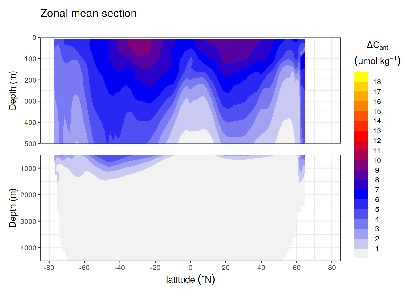
[[2]]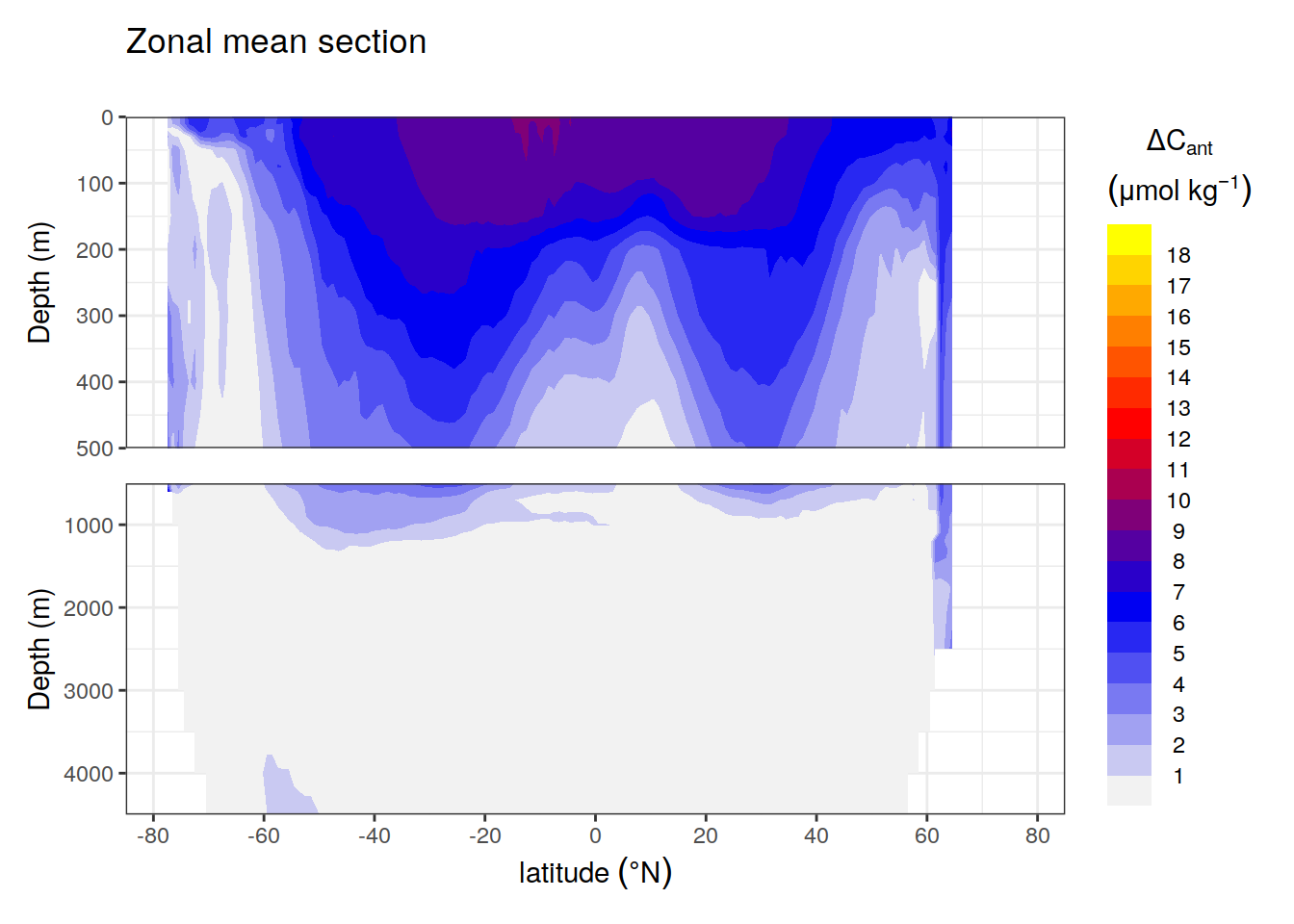
2.1 Calculation
To adjust observation-based C* values to the reference year of each observation period, we assume a transient steady state change of cant between the time of sampling the reference year. The adjustment requires an approximation of the cant concentration at the reference year. We approximate this concentration by adding the delta cant signal estimated by Gruber et al (2019) to the “base line” total cant concentration determined for 1994 by Sabine et al (2004):
Cant(tref) = S04 + (tref-1994)/13 * G19
This way, we use exactly S04+G19 for tref=2007. For all other tref we scale Cant with the observed anomalous change over the 1994-2007 period, rather than assuming a transient steady state. However, one assumes a linear behaviour of the anomalous change over time, which might be wrong in particular for the years past 2007.
For the model data, we perform the adjustment based on the total Cant estimate for 1994, and the delta Cant estimate for 1994 - 2007.
# assign reference year
GLODAP <- full_join(GLODAP, tref)

# extract atm pCO2 at reference year
co2_atm_tref <- right_join(co2_atm, tref %>% rename(year = median_year)) %>%
  select(-year) %>%
  rename(pCO2_tref = pCO2)

# merge atm pCO2 at tref with GLODAP
GLODAP <- full_join(GLODAP, co2_atm_tref)
rm(co2_atm)

# calculate cstar for reference year
GLODAP <- GLODAP %>%
  mutate(
    cstar_tref_delta =
      ((pCO2 - pCO2_tref) / (pCO2_tref - params_local$preind_atm_pCO2)) * cant_pos,
    cstar_tref = cstar - cstar_tref_delta)
sessionInfo()R version 4.0.3 (2020-10-10)
Platform: x86_64-pc-linux-gnu (64-bit)
Running under: openSUSE Leap 15.2
Matrix products: default
BLAS: /usr/local/R-4.0.3/lib64/R/lib/libRblas.so
LAPACK: /usr/local/R-4.0.3/lib64/R/lib/libRlapack.so
locale:
[1] LC_CTYPE=en_US.UTF-8 LC_NUMERIC=C
[3] LC_TIME=en_US.UTF-8 LC_COLLATE=en_US.UTF-8
[5] LC_MONETARY=en_US.UTF-8 LC_MESSAGES=en_US.UTF-8
[7] LC_PAPER=en_US.UTF-8 LC_NAME=C
[9] LC_ADDRESS=C LC_TELEPHONE=C
[11] LC_MEASUREMENT=en_US.UTF-8 LC_IDENTIFICATION=C
attached base packages:
[1] stats graphics grDevices utils datasets methods base
other attached packages:
[1] metR_0.9.0 scico_1.2.0 patchwork_1.1.1 collapse_1.5.0
[5] forcats_0.5.0 stringr_1.4.0 dplyr_1.0.5 purrr_0.3.4
[9] readr_1.4.0 tidyr_1.1.2 tibble_3.0.4 ggplot2_3.3.3
[13] tidyverse_1.3.0 workflowr_1.6.2
loaded via a namespace (and not attached):
[1] Rcpp_1.0.5 here_0.1 lattice_0.20-41
[4] lubridate_1.7.9 assertthat_0.2.1 rprojroot_2.0.2
[7] digest_0.6.27 R6_2.5.0 cellranger_1.1.0
[10] backports_1.1.10 reprex_0.3.0 evaluate_0.14
[13] httr_1.4.2 pillar_1.4.7 rlang_0.4.10
[16] readxl_1.3.1 data.table_1.13.2 rstudioapi_0.11
[19] whisker_0.4 blob_1.2.1 Matrix_1.2-18
[22] checkmate_2.0.0 rmarkdown_2.5 labeling_0.4.2
[25] RcppEigen_0.3.3.7.0 munsell_0.5.0 broom_0.7.5
[28] compiler_4.0.3 httpuv_1.5.4 modelr_0.1.8
[31] xfun_0.18 pkgconfig_2.0.3 htmltools_0.5.0
[34] tidyselect_1.1.0 fansi_0.4.1 crayon_1.3.4
[37] dbplyr_1.4.4 withr_2.3.0 later_1.1.0.1
[40] grid_4.0.3 jsonlite_1.7.1 gtable_0.3.0
[43] lifecycle_1.0.0 DBI_1.1.0 git2r_0.27.1
[46] magrittr_1.5 scales_1.1.1 cli_2.1.0
[49] stringi_1.5.3 farver_2.0.3 fs_1.5.0
[52] promises_1.1.1 RcppArmadillo_0.10.1.2.0 xml2_1.3.2
[55] ellipsis_0.3.1 generics_0.0.2 vctrs_0.3.5
[58] tools_4.0.3 glue_1.4.2 hms_0.5.3
[61] parallel_4.0.3 yaml_2.2.1 colorspace_1.4-1
[64] isoband_0.2.2 rvest_0.3.6 knitr_1.30
[67] haven_2.3.1