FESOM-REcoM
Jens Daniel Müller
24 May, 2024
Last updated: 2024-05-24
Checks: 7 0
Knit directory:
heatwave_co2_flux_2023/analysis/
This reproducible R Markdown analysis was created with workflowr (version 1.7.0). The Checks tab describes the reproducibility checks that were applied when the results were created. The Past versions tab lists the development history.
Great! Since the R Markdown file has been committed to the Git repository, you know the exact version of the code that produced these results.
Great job! The global environment was empty. Objects defined in the global environment can affect the analysis in your R Markdown file in unknown ways. For reproduciblity it’s best to always run the code in an empty environment.
The command set.seed(20240307) was run prior to running
the code in the R Markdown file. Setting a seed ensures that any results
that rely on randomness, e.g. subsampling or permutations, are
reproducible.
Great job! Recording the operating system, R version, and package versions is critical for reproducibility.
Nice! There were no cached chunks for this analysis, so you can be confident that you successfully produced the results during this run.
Great job! Using relative paths to the files within your workflowr project makes it easier to run your code on other machines.
Great! You are using Git for version control. Tracking code development and connecting the code version to the results is critical for reproducibility.
The results in this page were generated with repository version e2d6743. See the Past versions tab to see a history of the changes made to the R Markdown and HTML files.
Note that you need to be careful to ensure that all relevant files for
the analysis have been committed to Git prior to generating the results
(you can use wflow_publish or
wflow_git_commit). workflowr only checks the R Markdown
file, but you know if there are other scripts or data files that it
depends on. Below is the status of the Git repository when the results
were generated:
Ignored files:
    Ignored:    .Rhistory
    Ignored:    .Rproj.user/
    Ignored:    data/

Untracked files:
    Untracked:  figure/2023_absolute_means_and_integrals_global-1.png
    Untracked:  figure/2023_absolute_means_and_integrals_key_biomes-1.png
    Untracked:  figure/2023_absolute_means_and_integrals_key_biomes-2.png
    Untracked:  figure/2023_absolute_means_and_integrals_key_biomes-3.png
    Untracked:  figure/2023_absolute_means_and_integrals_key_biomes-4.png
    Untracked:  figure/2023_absolute_means_and_integrals_key_biomes_super-1.png
    Untracked:  figure/2023_absolute_means_and_integrals_key_biomes_super-2.png
    Untracked:  figure/2023_absolute_means_and_integrals_overview_biomes-1.png
    Untracked:  figure/2023_absolute_means_and_integrals_overview_biomes_super-1.png
    Untracked:  figure/2023_annual_mean_maps-10.png
    Untracked:  figure/2023_annual_mean_maps-11.png
    Untracked:  figure/2023_annual_mean_maps-12.png
    Untracked:  figure/2023_annual_mean_maps-13.png
    Untracked:  figure/2023_annual_mean_maps-14.png
    Untracked:  figure/2023_annual_mean_maps-15.png
    Untracked:  figure/2023_annual_mean_maps-16.png
    Untracked:  figure/2023_annual_mean_maps-17.png
    Untracked:  figure/2023_annual_mean_maps-6.png
    Untracked:  figure/2023_annual_mean_maps-7.png
    Untracked:  figure/2023_annual_mean_maps-8.png
    Untracked:  figure/2023_annual_mean_maps-9.png
    Untracked:  figure/2023_annual_mean_trends-1.png
    Untracked:  figure/2023_annual_mean_trends-2.png
    Untracked:  figure/2023_annual_mean_trends-3.png
    Untracked:  figure/2023_annual_mean_trends-4.png
    Untracked:  figure/2023_annual_mean_trends-5.png
    Untracked:  figure/2023_annual_mean_trends-6.png
    Untracked:  figure/2023_annual_mean_trends-7.png
    Untracked:  figure/2023_anomalies_correlation_absolute_biome_monthly-1.png
    Untracked:  figure/2023_anomalies_correlation_absolute_biome_monthly-10.png
    Untracked:  figure/2023_anomalies_correlation_absolute_biome_monthly-11.png
    Untracked:  figure/2023_anomalies_correlation_absolute_biome_monthly-12.png
    Untracked:  figure/2023_anomalies_correlation_absolute_biome_monthly-13.png
    Untracked:  figure/2023_anomalies_correlation_absolute_biome_monthly-14.png
    Untracked:  figure/2023_anomalies_correlation_absolute_biome_monthly-15.png
    Untracked:  figure/2023_anomalies_correlation_absolute_biome_monthly-16.png
    Untracked:  figure/2023_anomalies_correlation_absolute_biome_monthly-17.png
    Untracked:  figure/2023_anomalies_correlation_absolute_biome_monthly-2.png
    Untracked:  figure/2023_anomalies_correlation_absolute_biome_monthly-3.png
    Untracked:  figure/2023_anomalies_correlation_absolute_biome_monthly-4.png
    Untracked:  figure/2023_anomalies_correlation_absolute_biome_monthly-5.png
    Untracked:  figure/2023_anomalies_correlation_absolute_biome_monthly-6.png
    Untracked:  figure/2023_anomalies_correlation_absolute_biome_monthly-7.png
    Untracked:  figure/2023_anomalies_correlation_absolute_biome_monthly-8.png
    Untracked:  figure/2023_anomalies_correlation_absolute_biome_monthly-9.png
    Untracked:  figure/2023_anomalies_correlation_absolute_global_annual-1.png
    Untracked:  figure/2023_anomalies_correlation_absolute_global_monthly-1.png
    Untracked:  figure/2023_anomalies_correlation_absolute_super_biome_monthly-1.png
    Untracked:  figure/2023_anomalies_correlation_absolute_super_biome_monthly-10.png
    Untracked:  figure/2023_anomalies_correlation_absolute_super_biome_monthly-11.png
    Untracked:  figure/2023_anomalies_correlation_absolute_super_biome_monthly-12.png
    Untracked:  figure/2023_anomalies_correlation_absolute_super_biome_monthly-13.png
    Untracked:  figure/2023_anomalies_correlation_absolute_super_biome_monthly-14.png
    Untracked:  figure/2023_anomalies_correlation_absolute_super_biome_monthly-15.png
    Untracked:  figure/2023_anomalies_correlation_absolute_super_biome_monthly-16.png
    Untracked:  figure/2023_anomalies_correlation_absolute_super_biome_monthly-17.png
    Untracked:  figure/2023_anomalies_correlation_absolute_super_biome_monthly-2.png
    Untracked:  figure/2023_anomalies_correlation_absolute_super_biome_monthly-3.png
    Untracked:  figure/2023_anomalies_correlation_absolute_super_biome_monthly-4.png
    Untracked:  figure/2023_anomalies_correlation_absolute_super_biome_monthly-5.png
    Untracked:  figure/2023_anomalies_correlation_absolute_super_biome_monthly-6.png
    Untracked:  figure/2023_anomalies_correlation_absolute_super_biome_monthly-7.png
    Untracked:  figure/2023_anomalies_correlation_absolute_super_biome_monthly-8.png
    Untracked:  figure/2023_anomalies_correlation_absolute_super_biome_monthly-9.png
    Untracked:  figure/2023_anomalies_correlation_realtive_to_spread_monthly-1.png
    Untracked:  figure/2023_anomalies_correlation_realtive_to_spread_monthly-10.png
    Untracked:  figure/2023_anomalies_correlation_realtive_to_spread_monthly-11.png
    Untracked:  figure/2023_anomalies_correlation_realtive_to_spread_monthly-12.png
    Untracked:  figure/2023_anomalies_correlation_realtive_to_spread_monthly-13.png
    Untracked:  figure/2023_anomalies_correlation_realtive_to_spread_monthly-14.png
    Untracked:  figure/2023_anomalies_correlation_realtive_to_spread_monthly-15.png
    Untracked:  figure/2023_anomalies_correlation_realtive_to_spread_monthly-16.png
    Untracked:  figure/2023_anomalies_correlation_realtive_to_spread_monthly-17.png
    Untracked:  figure/2023_anomalies_correlation_realtive_to_spread_monthly-2.png
    Untracked:  figure/2023_anomalies_correlation_realtive_to_spread_monthly-3.png
    Untracked:  figure/2023_anomalies_correlation_realtive_to_spread_monthly-4.png
    Untracked:  figure/2023_anomalies_correlation_realtive_to_spread_monthly-5.png
    Untracked:  figure/2023_anomalies_correlation_realtive_to_spread_monthly-6.png
    Untracked:  figure/2023_anomalies_correlation_realtive_to_spread_monthly-7.png
    Untracked:  figure/2023_anomalies_correlation_realtive_to_spread_monthly-8.png
    Untracked:  figure/2023_anomalies_correlation_realtive_to_spread_monthly-9.png
    Untracked:  figure/2023_anomalies_from_annual_mean_trends_key_biomes-1.png
    Untracked:  figure/2023_anomalies_from_annual_mean_trends_key_biomes-2.png
    Untracked:  figure/2023_anomalies_from_annual_mean_trends_key_biomes-3.png
    Untracked:  figure/2023_anomalies_from_annual_mean_trends_key_biomes-4.png
    Untracked:  figure/2023_anomalies_from_annual_mean_trends_key_biomes_super-1.png
    Untracked:  figure/2023_anomalies_from_annual_mean_trends_key_biomes_super-2.png
    Untracked:  figure/2023_anomalies_from_annual_mean_trends_overview-1.png
    Untracked:  figure/2023_anomalies_from_annual_mean_trends_overview-2.png
    Untracked:  figure/2023_anomalies_from_annual_mean_trends_overview-3.png
    Untracked:  figure/2023_anomalies_from_monthly_mean_trends__key_biomes_overview-1.png
    Untracked:  figure/2023_anomalies_from_monthly_mean_trends_biomes_super-1.png
    Untracked:  figure/2023_anomalies_from_monthly_mean_trends_biomes_super-2.png
    Untracked:  figure/2023_anomalies_from_monthly_mean_trends_biomes_super_overview-1.png
    Untracked:  figure/2023_anomalies_from_monthly_mean_trends_global-1.png
    Untracked:  figure/2023_anomalies_from_monthly_mean_trends_global-2.png
    Untracked:  figure/2023_anomalies_from_monthly_mean_trends_global-3.png
    Untracked:  figure/2023_anomalies_from_monthly_mean_trends_key_biomes-1.png
    Untracked:  figure/2023_anomalies_from_monthly_mean_trends_key_biomes-2.png
    Untracked:  figure/2023_anomalies_from_monthly_mean_trends_key_biomes-3.png
    Untracked:  figure/2023_anomalies_from_monthly_mean_trends_key_biomes-4.png
    Untracked:  figure/2023_anomaly_annual_mean_maps-1.png
    Untracked:  figure/2023_anomaly_annual_mean_maps-10.png
    Untracked:  figure/2023_anomaly_annual_mean_maps-11.png
    Untracked:  figure/2023_anomaly_annual_mean_maps-12.png
    Untracked:  figure/2023_anomaly_annual_mean_maps-13.png
    Untracked:  figure/2023_anomaly_annual_mean_maps-14.png
    Untracked:  figure/2023_anomaly_annual_mean_maps-15.png
    Untracked:  figure/2023_anomaly_annual_mean_maps-16.png
    Untracked:  figure/2023_anomaly_annual_mean_maps-17.png
    Untracked:  figure/2023_anomaly_annual_mean_maps-2.png
    Untracked:  figure/2023_anomaly_annual_mean_maps-3.png
    Untracked:  figure/2023_anomaly_annual_mean_maps-4.png
    Untracked:  figure/2023_anomaly_annual_mean_maps-5.png
    Untracked:  figure/2023_anomaly_annual_mean_maps-6.png
    Untracked:  figure/2023_anomaly_annual_mean_maps-7.png
    Untracked:  figure/2023_anomaly_annual_mean_maps-8.png
    Untracked:  figure/2023_anomaly_annual_mean_maps-9.png
    Untracked:  figure/2023_anomaly_monthly_mean_maps-1.png
    Untracked:  figure/2023_anomaly_monthly_mean_maps-10.png
    Untracked:  figure/2023_anomaly_monthly_mean_maps-11.png
    Untracked:  figure/2023_anomaly_monthly_mean_maps-12.png
    Untracked:  figure/2023_anomaly_monthly_mean_maps-13.png
    Untracked:  figure/2023_anomaly_monthly_mean_maps-14.png
    Untracked:  figure/2023_anomaly_monthly_mean_maps-15.png
    Untracked:  figure/2023_anomaly_monthly_mean_maps-16.png
    Untracked:  figure/2023_anomaly_monthly_mean_maps-17.png
    Untracked:  figure/2023_anomaly_monthly_mean_maps-2.png
    Untracked:  figure/2023_anomaly_monthly_mean_maps-3.png
    Untracked:  figure/2023_anomaly_monthly_mean_maps-4.png
    Untracked:  figure/2023_anomaly_monthly_mean_maps-5.png
    Untracked:  figure/2023_anomaly_monthly_mean_maps-6.png
    Untracked:  figure/2023_anomaly_monthly_mean_maps-7.png
    Untracked:  figure/2023_anomaly_monthly_mean_maps-8.png
    Untracked:  figure/2023_anomaly_monthly_mean_maps-9.png
    Untracked:  figure/2023_anomaly_profiles-1.png
    Untracked:  figure/2023_anomaly_profiles-2.png
    Untracked:  figure/2023_anomaly_profiles-3.png
    Untracked:  figure/2023_anomaly_profiles-4.png
    Untracked:  figure/2023_anomaly_zonal_mean_sections-1.png
    Untracked:  figure/2023_anomaly_zonal_mean_sections-2.png
    Untracked:  figure/2023_anomaly_zonal_mean_sections-3.png
    Untracked:  figure/2023_anomaly_zonal_mean_sections-4.png
    Untracked:  figure/2023_change_annual_mean_maps-1.png
    Untracked:  figure/2023_change_annual_mean_maps-10.png
    Untracked:  figure/2023_change_annual_mean_maps-11.png
    Untracked:  figure/2023_change_annual_mean_maps-12.png
    Untracked:  figure/2023_change_annual_mean_maps-13.png
    Untracked:  figure/2023_change_annual_mean_maps-14.png
    Untracked:  figure/2023_change_annual_mean_maps-15.png
    Untracked:  figure/2023_change_annual_mean_maps-16.png
    Untracked:  figure/2023_change_annual_mean_maps-17.png
    Untracked:  figure/2023_change_annual_mean_maps-2.png
    Untracked:  figure/2023_change_annual_mean_maps-3.png
    Untracked:  figure/2023_change_annual_mean_maps-4.png
    Untracked:  figure/2023_change_annual_mean_maps-5.png
    Untracked:  figure/2023_change_annual_mean_maps-6.png
    Untracked:  figure/2023_change_annual_mean_maps-7.png
    Untracked:  figure/2023_change_annual_mean_maps-8.png
    Untracked:  figure/2023_change_annual_mean_maps-9.png
    Untracked:  figure/2023_change_monthly_mean_maps-1.png
    Untracked:  figure/2023_change_monthly_mean_maps-10.png
    Untracked:  figure/2023_change_monthly_mean_maps-11.png
    Untracked:  figure/2023_change_monthly_mean_maps-12.png
    Untracked:  figure/2023_change_monthly_mean_maps-13.png
    Untracked:  figure/2023_change_monthly_mean_maps-14.png
    Untracked:  figure/2023_change_monthly_mean_maps-15.png
    Untracked:  figure/2023_change_monthly_mean_maps-16.png
    Untracked:  figure/2023_change_monthly_mean_maps-17.png
    Untracked:  figure/2023_change_monthly_mean_maps-2.png
    Untracked:  figure/2023_change_monthly_mean_maps-3.png
    Untracked:  figure/2023_change_monthly_mean_maps-4.png
    Untracked:  figure/2023_change_monthly_mean_maps-5.png
    Untracked:  figure/2023_change_monthly_mean_maps-6.png
    Untracked:  figure/2023_change_monthly_mean_maps-7.png
    Untracked:  figure/2023_change_monthly_mean_maps-8.png
    Untracked:  figure/2023_change_monthly_mean_maps-9.png
    Untracked:  figure/2023_hovmoeller_annual_anomaly-1.png
    Untracked:  figure/2023_hovmoeller_annual_anomaly-10.png
    Untracked:  figure/2023_hovmoeller_annual_anomaly-11.png
    Untracked:  figure/2023_hovmoeller_annual_anomaly-12.png
    Untracked:  figure/2023_hovmoeller_annual_anomaly-13.png
    Untracked:  figure/2023_hovmoeller_annual_anomaly-14.png
    Untracked:  figure/2023_hovmoeller_annual_anomaly-15.png
    Untracked:  figure/2023_hovmoeller_annual_anomaly-16.png
    Untracked:  figure/2023_hovmoeller_annual_anomaly-17.png
    Untracked:  figure/2023_hovmoeller_annual_anomaly-18.png
    Untracked:  figure/2023_hovmoeller_annual_anomaly-2.png
    Untracked:  figure/2023_hovmoeller_annual_anomaly-3.png
    Untracked:  figure/2023_hovmoeller_annual_anomaly-4.png
    Untracked:  figure/2023_hovmoeller_annual_anomaly-5.png
    Untracked:  figure/2023_hovmoeller_annual_anomaly-6.png
    Untracked:  figure/2023_hovmoeller_annual_anomaly-7.png
    Untracked:  figure/2023_hovmoeller_annual_anomaly-8.png
    Untracked:  figure/2023_hovmoeller_annual_anomaly-9.png
    Untracked:  figure/2023_hovmoeller_monthly_anomalies-1.png
    Untracked:  figure/2023_hovmoeller_monthly_anomalies-10.png
    Untracked:  figure/2023_hovmoeller_monthly_anomalies-11.png
    Untracked:  figure/2023_hovmoeller_monthly_anomalies-12.png
    Untracked:  figure/2023_hovmoeller_monthly_anomalies-13.png
    Untracked:  figure/2023_hovmoeller_monthly_anomalies-14.png
    Untracked:  figure/2023_hovmoeller_monthly_anomalies-15.png
    Untracked:  figure/2023_hovmoeller_monthly_anomalies-16.png
    Untracked:  figure/2023_hovmoeller_monthly_anomalies-17.png
    Untracked:  figure/2023_hovmoeller_monthly_anomalies-18.png
    Untracked:  figure/2023_hovmoeller_monthly_anomalies-2.png
    Untracked:  figure/2023_hovmoeller_monthly_anomalies-3.png
    Untracked:  figure/2023_hovmoeller_monthly_anomalies-4.png
    Untracked:  figure/2023_hovmoeller_monthly_anomalies-5.png
    Untracked:  figure/2023_hovmoeller_monthly_anomalies-6.png
    Untracked:  figure/2023_hovmoeller_monthly_anomalies-7.png
    Untracked:  figure/2023_hovmoeller_monthly_anomalies-8.png
    Untracked:  figure/2023_hovmoeller_monthly_anomalies-9.png
    Untracked:  figure/2023_hovmoeller_monthly_anomalies_recent_years-1.png
    Untracked:  figure/2023_hovmoeller_monthly_anomalies_recent_years-10.png
    Untracked:  figure/2023_hovmoeller_monthly_anomalies_recent_years-11.png
    Untracked:  figure/2023_hovmoeller_monthly_anomalies_recent_years-12.png
    Untracked:  figure/2023_hovmoeller_monthly_anomalies_recent_years-13.png
    Untracked:  figure/2023_hovmoeller_monthly_anomalies_recent_years-14.png
    Untracked:  figure/2023_hovmoeller_monthly_anomalies_recent_years-15.png
    Untracked:  figure/2023_hovmoeller_monthly_anomalies_recent_years-16.png
    Untracked:  figure/2023_hovmoeller_monthly_anomalies_recent_years-17.png
    Untracked:  figure/2023_hovmoeller_monthly_anomalies_recent_years-18.png
    Untracked:  figure/2023_hovmoeller_monthly_anomalies_recent_years-2.png
    Untracked:  figure/2023_hovmoeller_monthly_anomalies_recent_years-3.png
    Untracked:  figure/2023_hovmoeller_monthly_anomalies_recent_years-4.png
    Untracked:  figure/2023_hovmoeller_monthly_anomalies_recent_years-5.png
    Untracked:  figure/2023_hovmoeller_monthly_anomalies_recent_years-6.png
    Untracked:  figure/2023_hovmoeller_monthly_anomalies_recent_years-7.png
    Untracked:  figure/2023_hovmoeller_monthly_anomalies_recent_years-8.png
    Untracked:  figure/2023_hovmoeller_monthly_anomalies_recent_years-9.png
    Untracked:  figure/2023_monthly_mean_maps-10.png
    Untracked:  figure/2023_monthly_mean_maps-11.png
    Untracked:  figure/2023_monthly_mean_maps-12.png
    Untracked:  figure/2023_monthly_mean_maps-13.png
    Untracked:  figure/2023_monthly_mean_maps-14.png
    Untracked:  figure/2023_monthly_mean_maps-15.png
    Untracked:  figure/2023_monthly_mean_maps-16.png
    Untracked:  figure/2023_monthly_mean_maps-17.png
    Untracked:  figure/2023_monthly_mean_maps-6.png
    Untracked:  figure/2023_monthly_mean_maps-7.png
    Untracked:  figure/2023_monthly_mean_maps-8.png
    Untracked:  figure/2023_monthly_mean_maps-9.png
    Untracked:  figure/2023_monthly_mean_trends-1.png
    Untracked:  figure/2023_monthly_mean_trends-2.png
    Untracked:  figure/2023_monthly_mean_trends-3.png
    Untracked:  figure/2023_monthly_mean_trends-4.png
    Untracked:  figure/hovmoeller_annual_absolute-10.png
    Untracked:  figure/hovmoeller_annual_absolute-11.png
    Untracked:  figure/hovmoeller_annual_absolute-12.png
    Untracked:  figure/hovmoeller_annual_absolute-13.png
    Untracked:  figure/hovmoeller_annual_absolute-14.png
    Untracked:  figure/hovmoeller_annual_absolute-15.png
    Untracked:  figure/hovmoeller_annual_absolute-16.png
    Untracked:  figure/hovmoeller_annual_absolute-17.png
    Untracked:  figure/hovmoeller_annual_absolute-18.png
    Untracked:  figure/hovmoeller_annual_absolute-6.png
    Untracked:  figure/hovmoeller_annual_absolute-7.png
    Untracked:  figure/hovmoeller_annual_absolute-8.png
    Untracked:  figure/hovmoeller_annual_absolute-9.png
    Untracked:  figure/hovmoeller_monthly_absolute-10.png
    Untracked:  figure/hovmoeller_monthly_absolute-11.png
    Untracked:  figure/hovmoeller_monthly_absolute-12.png
    Untracked:  figure/hovmoeller_monthly_absolute-13.png
    Untracked:  figure/hovmoeller_monthly_absolute-14.png
    Untracked:  figure/hovmoeller_monthly_absolute-15.png
    Untracked:  figure/hovmoeller_monthly_absolute-16.png
    Untracked:  figure/hovmoeller_monthly_absolute-17.png
    Untracked:  figure/hovmoeller_monthly_absolute-18.png
    Untracked:  figure/hovmoeller_monthly_absolute-6.png
    Untracked:  figure/hovmoeller_monthly_absolute-7.png
    Untracked:  figure/hovmoeller_monthly_absolute-8.png
    Untracked:  figure/hovmoeller_monthly_absolute-9.png

Unstaged changes:
    Modified:   analysis/biomes.Rmd
    Modified:   analysis/child/pCO2_product_analysis.Rmd
    Modified:   analysis/child/pCO2_product_preprocessing.Rmd
    Modified:   analysis/child/pCO2_product_synopsis.Rmd
    Modified:   code/Workflowr_project_managment.R
    Modified:   figure/2023_annual_mean_maps-1.png
    Modified:   figure/2023_annual_mean_maps-2.png
    Modified:   figure/2023_annual_mean_maps-3.png
    Modified:   figure/2023_annual_mean_maps-4.png
    Modified:   figure/2023_annual_mean_maps-5.png
    Modified:   figure/2023_monthly_mean_maps-1.png
    Modified:   figure/2023_monthly_mean_maps-2.png
    Modified:   figure/2023_monthly_mean_maps-3.png
    Modified:   figure/2023_monthly_mean_maps-4.png
    Modified:   figure/2023_monthly_mean_maps-5.png
    Modified:   figure/hovmoeller_annual_absolute-1.png
    Modified:   figure/hovmoeller_annual_absolute-2.png
    Modified:   figure/hovmoeller_annual_absolute-3.png
    Modified:   figure/hovmoeller_annual_absolute-4.png
    Modified:   figure/hovmoeller_annual_absolute-5.png
    Modified:   figure/hovmoeller_monthly_absolute-1.png
    Modified:   figure/hovmoeller_monthly_absolute-2.png
    Modified:   figure/hovmoeller_monthly_absolute-3.png
    Modified:   figure/hovmoeller_monthly_absolute-4.png
    Modified:   figure/hovmoeller_monthly_absolute-5.png
Note that any generated files, e.g. HTML, png, CSS, etc., are not included in this status report because it is ok for generated content to have uncommitted changes.
These are the previous versions of the repository in which changes were
made to the R Markdown (analysis/FESOM_REcoM.Rmd) and HTML
(docs/FESOM_REcoM.html) files. If you’ve configured a
remote Git repository (see ?wflow_git_remote), click on the
hyperlinks in the table below to view the files as they were in that
past version.
| File | Version | Author | Date | Message |
|---|---|---|---|---|
| Rmd | e2d6743 | jens-daniel-mueller | 2024-05-24 | talk included, variable names adapted, monthly anomaly profiles addded |
| html | 4a4e4df | jens-daniel-mueller | 2024-05-24 | Build site. |
| html | 054921b | jens-daniel-mueller | 2024-05-23 | Build site. |
| Rmd | 8331c52 | jens-daniel-mueller | 2024-05-23 | read 3D ocean interior fields |
| html | 38f6f6e | jens-daniel-mueller | 2024-05-22 | Build site. |
| Rmd | a7f3127 | jens-daniel-mueller | 2024-05-22 | read bgc surface variables |
| html | be285dc | jens-daniel-mueller | 2024-05-21 | Build site. |
| html | 51df30d | jens-daniel-mueller | 2024-05-15 | Build site. |
| Rmd | 981d5e1 | jens-daniel-mueller | 2024-05-15 | kw K0 product included, mean flux densities computed |
| html | 009791f | jens-daniel-mueller | 2024-05-14 | Build site. |
| html | 3b5d16b | jens-daniel-mueller | 2024-05-13 | Build site. |
| Rmd | 1e1dee5 | jens-daniel-mueller | 2024-05-13 | pco2 to fco2 conversions, changed output files |
| html | 13225ec | jens-daniel-mueller | 2024-05-08 | Build site. |
| Rmd | fb237ae | jens-daniel-mueller | 2024-05-08 | 2016 and 1998 included |
| html | fb21e78 | jens-daniel-mueller | 2024-05-08 | Build site. |
| Rmd | 51196a6 | jens-daniel-mueller | 2024-05-08 | units fixed |
| html | c7897dc | jens-daniel-mueller | 2024-05-08 | Build site. |
| Rmd | d77b01c | jens-daniel-mueller | 2024-05-08 | read new data |
| html | 7f9c687 | jens-daniel-mueller | 2024-04-23 | Build site. |
| html | ce4e2a6 | jens-daniel-mueller | 2024-04-17 | Build site. |
| Rmd | 6b3a080 | jens-daniel-mueller | 2024-04-17 | rebuild entire website with NRT_fco2residual |
center <- -160
boundary <- center + 180
target_crs <- paste0("+proj=robin +over +lon_0=", center)
# target_crs <- paste0("+proj=eqearth +over +lon_0=", center)
# target_crs <- paste0("+proj=eqearth +lon_0=", center)
# target_crs <- paste0("+proj=igh_o +lon_0=", center)

worldmap <- ne_countries(scale = 'small',
                         type = 'map_units',
                         returnclass = 'sf')

worldmap <- worldmap %>% st_break_antimeridian(lon_0 = center)
worldmap_trans <- st_transform(worldmap, crs = target_crs)

# ggplot() +
#   geom_sf(data = worldmap_trans)

coastline <- ne_coastline(scale = 'small', returnclass = "sf")
coastline <- st_break_antimeridian(coastline, lon_0 = 200)
coastline_trans <- st_transform(coastline, crs = target_crs)

# ggplot() +
#   geom_sf(data = worldmap_trans, fill = "grey", col="grey") +
#   geom_sf(data = coastline_trans)


bbox <- st_bbox(c(xmin = -180, xmax = 180, ymax = 65, ymin = -78), crs = st_crs(4326))
bbox <- st_as_sfc(bbox)
bbox_trans <- st_break_antimeridian(bbox, lon_0 = center)

bbox_graticules <- st_graticule(
  x = bbox_trans,
  crs = st_crs(bbox_trans),
  datum = st_crs(bbox_trans),
  lon = c(20, 20.001),
  lat = c(-78,65),
  ndiscr = 1e3,
  margin = 0.001
)

bbox_graticules_trans <- st_transform(bbox_graticules, crs = target_crs)
rm(worldmap, coastline, bbox, bbox_trans)

# ggplot() +
#   geom_sf(data = worldmap_trans, fill = "grey", col="grey") +
#   geom_sf(data = coastline_trans) +
#   geom_sf(data = bbox_graticules_trans)

lat_lim <- ext(bbox_graticules_trans)[c(3,4)]*1.002
lon_lim <- ext(bbox_graticules_trans)[c(1,2)]*1.005

# ggplot() +
#   geom_sf(data = worldmap_trans, fill = "grey90", col = "grey90") +
#   geom_sf(data = coastline_trans) +
#   geom_sf(data = bbox_graticules_trans, linewidth = 1) +
#   coord_sf(crs = target_crs,
#            ylim = lat_lim,
#            xlim = lon_lim,
#            expand = FALSE) +
#   theme(
#     panel.border = element_blank(),
#     axis.text = element_blank(),
#     axis.ticks = element_blank()
#   )

latitude_graticules <- st_graticule(
  x = bbox_graticules,
  crs = st_crs(bbox_graticules),
  datum = st_crs(bbox_graticules),
  lon = c(20, 20.001),
  lat = c(-60,-30,0,30,60),
  ndiscr = 1e3,
  margin = 0.001
)

latitude_graticules_trans <- st_transform(latitude_graticules, crs = target_crs)

latitude_labels <- data.frame(lat_label = c("60°N","30°N","Eq.","30°S","60°S"),
                 lat = c(60,30,0,-30,-60)-4, lon = c(35)-c(0,2,4,2,0))

latitude_labels <- st_as_sf(x = latitude_labels,
               coords = c("lon", "lat"),
               crs = "+proj=longlat")

latitude_labels_trans <- st_transform(latitude_labels, crs = target_crs)

# ggplot() +
#   geom_sf(data = worldmap_trans, fill = "grey", col = "grey") +
#   geom_sf(data = coastline_trans) +
#   geom_sf(data = bbox_graticules_trans) +
#   geom_sf(data = latitude_graticules_trans,
#           col = "grey60",
#           linewidth = 0.2) +
#   geom_sf_text(data = latitude_labels_trans,
#                aes(label = lat_label),
#                size = 3,
#                col = "grey60")
Read data
path_FESOM <-
  "/net/kryo/work/loher/GlobalMarineHeatwaves/AWI_FESOM2/"
library(ncdf4)
nc <-
nc_open(paste0(
path_FESOM,
"dissic_FESOM2_REcoM_A_1_gr_1980-2023_v20220716.nc"
))
print(nc)FESOM_files <- list.files(path = path_FESOM)
FESOM_files <-
FESOM_files[FESOM_files %>% str_detect(c(
"dissic_|no3|thetao|talk_"
))]
dates <- seq(ymd("1980-01-15"), ymd("2023-12-15"), "months")
for (i_FESOM_files in FESOM_files) {
# i_FESOM_files <- FESOM_files[1]
i_pco2_product_interior <-
read_mdim(paste0(path_FESOM,
i_FESOM_files))
i_pco2_product_interior <-
i_pco2_product_interior %>%
filter(Depth <= 500)
i_pco2_product_interior <-
st_set_dimensions(i_pco2_product_interior, 4, values = dates, names = "time")
if (exists("pco2_product_interior")) {
pco2_product_interior <-
c(pco2_product_interior,
i_pco2_product_interior)
}
if (!exists("pco2_product_interior")) {
pco2_product_interior <- i_pco2_product_interior
}
}
rm(FESOM_files, i_FESOM_files, i_pco2_product_interior)
# rm(pco2_product_interior)
pco2_product_interior <- pco2_product_interior %>%
as_tibble()
pco2_product_interior <- pco2_product_interior %>%
drop_na()
gc() used (Mb) gc trigger (Mb) max used (Mb)
Ncells 2876085 153.6 5463952 291.9 3968771 212.0
Vcells 3545394809 27049.3 10439830745 79649.6 9583098258 73113.3pco2_product_interior <-
pco2_product_interior %>%
rename(lat = Lat,
lon = Lon,
depth = Depth)
pco2_product_interior <-
pco2_product_interior %>%
mutate(
lon = if_else(lon < 20, lon + 360, lon),
no3 = no3 * 1.025e3,
dissic = dissic * 1.025e3,
talk = talk * 1.025e3
)
gc() used (Mb) gc trigger (Mb) max used (Mb)
Ncells 2905699 155.2 5463952 291.9 3968771 212.0
Vcells 3545456578 27049.7 10439830745 79649.6 9583098258 73113.3pco2_product_surf <-
pco2_product_interior %>%
filter(depth == min(depth))
gc() used (Mb) gc trigger (Mb) max used (Mb)
Ncells 2907898 155.3 5463952 291.9 3968771 212.0
Vcells 3722455365 28400.1 10439830745 79649.6 9583098258 73113.3FESOM_files <- list.files(path = path_FESOM)
FESOM_files <-
FESOM_files[FESOM_files %>% str_detect(c(
"alpha|chlos|fgco2|Kw|mld|fCO2atm|sfco2|sos|tos|intpp|dissicos|talkos"
))]
for (i_FESOM_files in FESOM_files) {
# i_FESOM_files <- FESOM_files[1]
i_pco2_product <-
read_ncdf(paste0(path_FESOM,
i_FESOM_files))
i_pco2_product <-
st_set_dimensions(i_pco2_product, 3, values = dates, names = "time")
if (exists("pco2_product")) {
pco2_product <-
c(pco2_product,
i_pco2_product)
}
if (!exists("pco2_product")) {
pco2_product <- i_pco2_product
}
}
rm(FESOM_files, i_FESOM_files, i_pco2_product)
# rm(pco2_product)
pco2_product <- pco2_product %>%
as_tibble()
pco2_product <-
pco2_product %>%
rename(lat = Lat,
lon = Lon) %>%
mutate(year = year(time),
month = month(time))
pco2_product <-
pco2_product %>%
rename(sol = alpha,
chl = chlos,
kw = Kw,
atm_fco2 = fCO2atm,
salinity = sos,
temperature = tos,
dissic = dissicos,
talk = talkos) %>%
mutate(
lon = if_else(lon < 20, lon + 360, lon),
chl = log10(chl * 1e6),
kw = kw * 60 * 60 * 24 * 365,
# mld = log10(-mld),
sol = sol * 1.025e3 * 1e-6,
fgco2 = -fgco2 * 60 * 60 * 24 * 365,
dfco2 = sfco2 - atm_fco2,
dissic = dissic * 1.025e3,
talk = talk * 1.025e3
)
pco2_product <-
pco2_product %>%
mutate(kw_sol = kw * sol)
pco2_product <-
full_join(pco2_product,
pco2_product_surf %>% select(-c(depth, thetao, dissic, talk)))
rm(pco2_product_surf)
gc() used (Mb) gc trigger (Mb) max used (Mb)
Ncells 2947360 157.5 5463952 291.9 5463952 291.9
Vcells 4229832636 32271.1 10439830745 79649.6 9583098258 73113.3# pco2_product %>%
# filter(time == max(time)) %>%
# select(lon, lat, temperature, sol, dissic) %>%
# ggplot(aes(lon, lat, fill = sol)) +
# geom_tile() +
# scale_fill_viridis_c()pCO2_product_preprocessing <-
knitr::knit_expand(file = here::here("analysis/child/pCO2_product_preprocessing.Rmd"),
product_name = "FESOM-REcoM")Preprocessing
# model <- TRUE
model <- str_detect('FESOM-REcoM', "FESOM-REcoM|ETHZ_CESM")
Load masks
biome_mask <-
  read_rds(here::here("data/biome_mask.rds"))

region_mask <-
  read_rds(here::here("data/region_mask.rds"))

map <-
  read_rds(here::here("data/map.rds"))

key_biomes <-
  read_rds(here::here("data/key_biomes.rds"))

super_biomes <-
  read_rds(here::here("data/super_biomes.rds"))

super_biome_mask <-
  read_rds(here::here("data/super_biome_mask.rds"))
Define labels and breaks
labels_breaks <- function(i_name) {

  if (i_name == "dco2") {
    i_legend_title <- "ΔpCO<sub>2</sub><br>(µatm)"
  }

  if (i_name == "dfco2") {
    i_legend_title <- "ΔfCO<sub>2</sub><br>(µatm)"
  }

  if (i_name == "atm_co2") {
    i_legend_title <- "pCO<sub>2,atm</sub><br>(µatm)"
  }

  if (i_name == "atm_fco2") {
    i_legend_title <- "fCO<sub>2,atm</sub><br>(µatm)"
  }

  if (i_name == "sol") {
    i_legend_title <- "K<sub>0</sub><br>(mol m<sup>-3</sup> µatm<sup>-1</sup>)"
  }

  if (i_name == "kw") {
    i_legend_title <- "k<sub>w</sub><br>(m yr<sup>-1</sup>)"
  }

  if (i_name == "kw_sol") {
    i_legend_title <- "k<sub>w</sub> K<sub>0</sub><br>(mol yr<sup>-1</sup> m<sup>-2</sup> µatm<sup>-1</sup>)"
  }

  if (i_name == "spco2") {
    i_legend_title <- "pCO<sub>2,ocean</sub><br>(µatm)"
  }

  if (i_name == "sfco2") {
    i_legend_title <- "fCO<sub>2,ocean</sub><br>(µatm)"
  }

  if (i_name == "intpp") {
    i_legend_title <- "NPP<sub>int</sub><br>(mol s<sup>-1</sup> m<sup>-2</sup>)"
  }

  if (i_name == "no3") {
    i_legend_title <- "NO<sub>3</sub><br>(μmol kg<sup>-1</sup>)"
  }

  if (i_name == "o2") {
    i_legend_title <- "O<sub>2</sub><br>(μmol kg<sup>-1</sup>)"
  }

  if (i_name == "dissic") {
    i_legend_title <- "DIC<br>(μmol kg<sup>-1</sup>)"
  }

  if (i_name == "talk") {
    i_legend_title <- "TA<br>(μmol kg<sup>-1</sup>)"
  }

  if (i_name == "sfco2_total") {
    i_legend_title <- "total"
  }

  if (i_name == "sfco2_therm") {
    i_legend_title <- "thermal"
  }

  if (i_name == "sfco2_nontherm") {
    i_legend_title <- "non-thermal"
  }

  if (i_name == "fgco2") {
    i_legend_title <- "FCO<sub>2</sub><br>(mol m<sup>-2</sup> yr<sup>-1</sup>)"
  }

  if (i_name == "fgco2_hov") {
    i_legend_title <- "FCO<sub>2</sub><br>(PgC deg<sup>-1</sup> yr<sup>-1</sup>)"
  }

  if (i_name == "fgco2_int") {
    i_legend_title <- "FCO<sub>2</sub><br>(PgC yr<sup>-1</sup>)"
  }

  if (i_name == "thetao") {
    i_legend_title <- "Temp.<br>(°C)"
  }

  if (i_name == "temperature") {
    i_legend_title <- "SST<br>(°C)"
  }

  if (i_name == "salinity") {
    i_legend_title <- "SSS"
  }

  if (i_name == "chl") {
    i_legend_title <- "lg(Chl-a)<br>(lg(mg m<sup>-3</sup>))"
  }

  if (i_name == "mld") {
    i_legend_title <- "MLD<br>(m)"
  }

  if (i_name == "press") {
    i_legend_title <- "pressure<sub>atm</sub><br>(Pa)"
  }

  if (i_name == "wind") {
    i_legend_title <- "Wind <br>(m sec<sup>-1</sup>)"
  }

  if (i_name == "SSH") {
    i_legend_title <- "SSH <br>(m)"
  }

  if (i_name == "fice") {
    i_legend_title <- "Sea ice <br>(%)"
  }


  if (i_name == "resid_fgco2") {
    i_legend_title <-
      "Observed"
  }

  if (i_name == "resid_fgco2_dfco2") {
    i_legend_title <-
      "ΔfCO<sub>2</sub>"
  }

  if (i_name == "resid_fgco2_kw_sol") {
    i_legend_title <-
      "k<sub>w</sub> K<sub>0</sub>"
  }

  if (i_name == "resid_fgco2_dfco2_kw_sol") {
    i_legend_title <-
      "k<sub>w</sub> K<sub>0</sub> X ΔfCO<sub>2</sub>"
  }

  if (i_name == "resid_fgco2_sum") {
    i_legend_title <-
      "∑"
  }

  if (i_name == "resid_fgco2_offset") {
    i_legend_title <-
      "Obs. - ∑"
  }

  all_labels_breaks <- lst(i_legend_title)

  return(all_labels_breaks)

}

x_axis_labels <-
  c(
    "dco2" = labels_breaks("dco2")$i_legend_title,
    "dfco2" = labels_breaks("dfco2")$i_legend_title,
    "atm_co2" = labels_breaks("atm_co2")$i_legend_title,
    "atm_fco2" = labels_breaks("atm_fco2")$i_legend_title,
    "sol" = labels_breaks("sol")$i_legend_title,
    "kw" = labels_breaks("kw")$i_legend_title,
    "kw_sol" = labels_breaks("kw_sol")$i_legend_title,
    "intpp" = labels_breaks("intpp")$i_legend_title,
    "no3" = labels_breaks("no3")$i_legend_title,
    "o2" = labels_breaks("o2")$i_legend_title,
    "dissic" = labels_breaks("dissic")$i_legend_title,
    "talk" = labels_breaks("talk")$i_legend_title,
    "spco2" = labels_breaks("spco2")$i_legend_title,
    "sfco2" = labels_breaks("sfco2")$i_legend_title,
    "sfco2_total" = labels_breaks("sfco2_total")$i_legend_title,
    "sfco2_therm" = labels_breaks("sfco2_therm")$i_legend_title,
    "sfco2_nontherm" = labels_breaks("sfco2_nontherm")$i_legend_title,
    "fgco2" = labels_breaks("fgco2")$i_legend_title,
    "fgco2_hov" = labels_breaks("fgco2_hov")$i_legend_title,
    "fgco2_int" = labels_breaks("fgco2_int")$i_legend_title,
    "thetao" = labels_breaks("thetao")$i_legend_title,
    "temperature" = labels_breaks("temperature")$i_legend_title,
    "salinity" = labels_breaks("salinity")$i_legend_title,
    "chl" = labels_breaks("chl")$i_legend_title,
    "mld" = labels_breaks("mld")$i_legend_title,
    "press" = labels_breaks("press")$i_legend_title,
    "wind" = labels_breaks("wind")$i_legend_title,
    "SSH" = labels_breaks("SSH")$i_legend_title,
    "fice" = labels_breaks("fice")$i_legend_title,
    "resid_fgco2" = labels_breaks("resid_fgco2")$i_legend_title,
    "resid_fgco2_dfco2" = labels_breaks("resid_fgco2_dfco2")$i_legend_title,
    "resid_fgco2_kw_sol" = labels_breaks("resid_fgco2_kw_sol")$i_legend_title,
    "resid_fgco2_dfco2_kw_sol" = labels_breaks("resid_fgco2_dfco2_kw_sol")$i_legend_title,
    "resid_fgco2_sum" = labels_breaks("resid_fgco2_sum")$i_legend_title,
    "resid_fgco2_offset" = labels_breaks("resid_fgco2_offset")$i_legend_title
  )
Analysis settings
name_quadratic_fit <- c("atm_co2", "atm_fco2", "spco2", "sfco2")

start_year <- 1990

name_divergent <- c("dco2", "dfco2", "fgco2", "fgco2_hov", "fgco2_int")
Data preprocessing
pco2_product <-
  pco2_product %>%
  filter(year >= start_year)
pco2_product_interior <-
pco2_product_interior %>%
filter(time >= ymd(paste0(start_year, "-01-01")))biome_mask <- biome_mask %>%
mutate(area = earth_surf(lat, lon))
pco2_product <-
full_join(pco2_product,
biome_mask)
# set all values outside biome mask to NA
pco2_product <-
pco2_product %>%
mutate(across(-c(lat, lon, time, area, year, month, biome),
~ if_else(is.na(biome), NA, .)))Compuations
# apply coarse grid

pco2_product_coarse <-
  m_grid_horizontal_coarse(pco2_product)

pco2_product_coarse <-
  pco2_product_coarse %>%
  select(-c(lon, lat, time, biome)) %>%
  group_by(year, month, lon_grid, lat_grid) %>%
  summarise(across(-area,
                   ~ weighted.mean(., area))) %>%
  ungroup() %>%
  rename(lon = lon_grid, lat = lat_grid)

pco2_product_coarse <-
  pco2_product_coarse %>%
  pivot_longer(-c(year, month, lon, lat)) %>%
  drop_na() %>%
  pivot_wider()

# compute annual means

pco2_product_coarse_annual <-
  pco2_product_coarse %>%
  select(-month) %>%
  group_by(year, lon, lat) %>%
  summarise(across(where(is.numeric),
                   ~ mean(.))) %>%
  ungroup()

pco2_product_coarse_annual <-
  pco2_product_coarse_annual %>%
  pivot_longer(-c(year, lon, lat))

## compute monthly means

pco2_product_coarse_monthly <-
  pco2_product_coarse %>%
  group_by(year, month, lon, lat) %>%
  summarise(across(where(is.numeric),
                   ~ mean(.))) %>%
  ungroup()

pco2_product_coarse_monthly <-
  pco2_product_coarse_monthly %>%
  pivot_longer(-c(year, month, lon, lat))
pco2_product_monthly_global <-
pco2_product %>%
filter(!is.na(fgco2)) %>%
mutate(fgco2_int = fgco2) %>%
select(-c(lon, lat, year, month, biome)) %>%
group_by(time) %>%
summarise(across(-c(fgco2_int, area),
~ weighted.mean(., area, na.rm = TRUE)),
across(fgco2_int,
~ sum(. * area, na.rm = TRUE) * 12.01 * 1e-15)) %>%
ungroup()
pco2_product_monthly_biome <-
pco2_product %>%
filter(!is.na(fgco2)) %>%
mutate(fgco2_int = fgco2) %>%
select(-c(lon, lat, year, month)) %>%
group_by(time, biome) %>%
summarise(across(-c(fgco2_int, area),
~ weighted.mean(., area, na.rm = TRUE)),
across(fgco2_int,
~ sum(. * area, na.rm = TRUE) * 12.01 * 1e-15)) %>%
ungroup()
pco2_product_monthly_biome_super <-
pco2_product %>%
filter(!is.na(fgco2)) %>%
mutate(fgco2_int = fgco2) %>%
mutate(
biome = case_when(
str_detect(biome, "NA-") ~ "North Atlantic",
str_detect(biome, "NP-") ~ "North Pacific",
str_detect(biome, "SO-") ~ "Southern Ocean",
TRUE ~ "other"
)
) %>%
filter(biome != "other") %>%
select(-c(lon, lat, year, month)) %>%
group_by(time, biome) %>%
summarise(across(-c(fgco2_int, area),
~ weighted.mean(., area, na.rm = TRUE)),
across(fgco2_int,
~ sum(. * area, na.rm = TRUE) * 12.01 * 1e-15)) %>%
ungroup()
pco2_product_monthly <-
bind_rows(pco2_product_monthly_global %>%
mutate(biome = "Global"),
pco2_product_monthly_biome,
pco2_product_monthly_biome_super)
rm(
pco2_product_monthly_global,
pco2_product_monthly_biome,
pco2_product_monthly_biome_super
)
pco2_product_monthly <-
pco2_product_monthly %>%
filter(!is.na(biome))
pco2_product_monthly <-
pco2_product_monthly %>%
mutate(year = year(time),
month = month(time),
.after = time)
pco2_product_monthly <-
pco2_product_monthly %>%
pivot_longer(-c(time, year, month, biome))pco2_product_interior <-
left_join(
biome_mask,
pco2_product_interior
)
pco2_product_profiles <- pco2_product_interior %>%
fselect(-c(lat, lon)) %>%
fgroup_by(biome, depth, time) %>% {
add_vars(fgroup_vars(., "unique"),
fmean(.,
w = area,
keep.w = FALSE,
keep.group_vars = FALSE))
}
pco2_product_profiles <-
pco2_product_profiles %>%
mutate(
year = year(time),
month = month(time)
)
gc() used (Mb) gc trigger (Mb) max used (Mb)
Ncells 3030744 161.9 52970018 2829.0 66212522 3536.2
Vcells 2614612122 19948.0 8351864596 63719.7 10432226898 79591.6pco2_product_interior <-
left_join(
region_mask,
pco2_product_interior %>% select(-c(biome, area))
)
pco2_product_zonal_mean <- pco2_product_interior %>%
fselect(-c(lon)) %>%
fgroup_by(region, depth, lat, time) %>% {
add_vars(fgroup_vars(., "unique"),
fmean(.,
keep.group_vars = FALSE))
}
pco2_product_zonal_mean <-
pco2_product_zonal_mean %>%
mutate(
year = year(time),
month = month(time)
)
gc() used (Mb) gc trigger (Mb) max used (Mb)
Ncells 3030807 161.9 42376015 2263.2 66212522 3536.2
Vcells 2440021165 18615.9 6681491677 50975.8 10432226898 79591.6# pco2_product_zonal_mean %>%
# filter(region == "atlantic",
# year == 2023,
# month == 1) %>%
# ggplot(aes(lat, depth, z = no3)) +
# geom_contour_filled() +
# scale_y_reverse() +
# scale_fill_viridis_d()
rm(pco2_product_interior)
gc() used (Mb) gc trigger (Mb) max used (Mb)
Ncells 3030847 161.9 33900812 1810.5 66212522 3536.2
Vcells 650582141 4963.6 5345193342 40780.6 10432226898 79591.6Absolute values
Hovmoeller plots
The following Hovmoeller plots show the value of each variable as provided through the pCO2 product. Hovmoeller plots are first presented as annual means, and than as monthly means.
Annual means
pco2_product_hovmoeller_monthly_annual <-
  pco2_product %>%
  mutate(fgco2_int = fgco2) %>%
  select(-c(lon, time, month, biome)) %>%
  group_by(year, lat) %>%
  summarise(across(-c(fgco2_int, area),
                   ~ weighted.mean(., area, na.rm = TRUE)),
            across(fgco2_int,
                   ~ sum(. * area, na.rm = TRUE) * 12.01 * 1e-15)) %>%
  ungroup() %>%
  rename(fgco2_hov = fgco2_int) %>%
  filter(fgco2_hov != 0)

pco2_product_hovmoeller_monthly_annual <-
  pco2_product_hovmoeller_monthly_annual %>%
  pivot_longer(-c(year, lat)) %>%
  drop_na()

pco2_product_hovmoeller_monthly_annual %>%
  filter(!(name %in% name_divergent)) %>%
  group_split(name) %>%
  # tail(5) %>%
  map(
    ~ ggplot(data = .x,
             aes(year, lat, fill = value)) +
      geom_raster() +
      scale_fill_viridis_c(name = labels_breaks(.x %>% distinct(name))) +
      theme(legend.title = element_markdown()) +
      coord_cartesian(expand = 0) +
      labs(title = "Annual means",
           y = "Latitude") +
      theme(axis.title.x = element_blank())
  )
[[1]]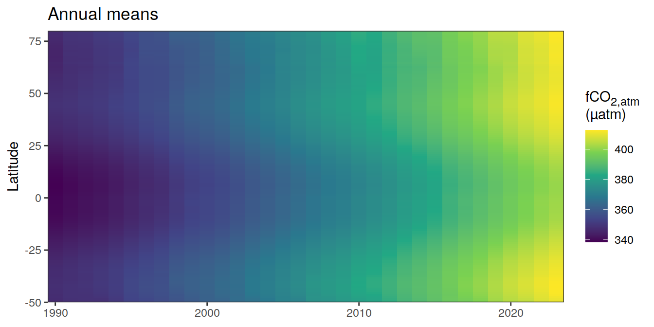
[[2]]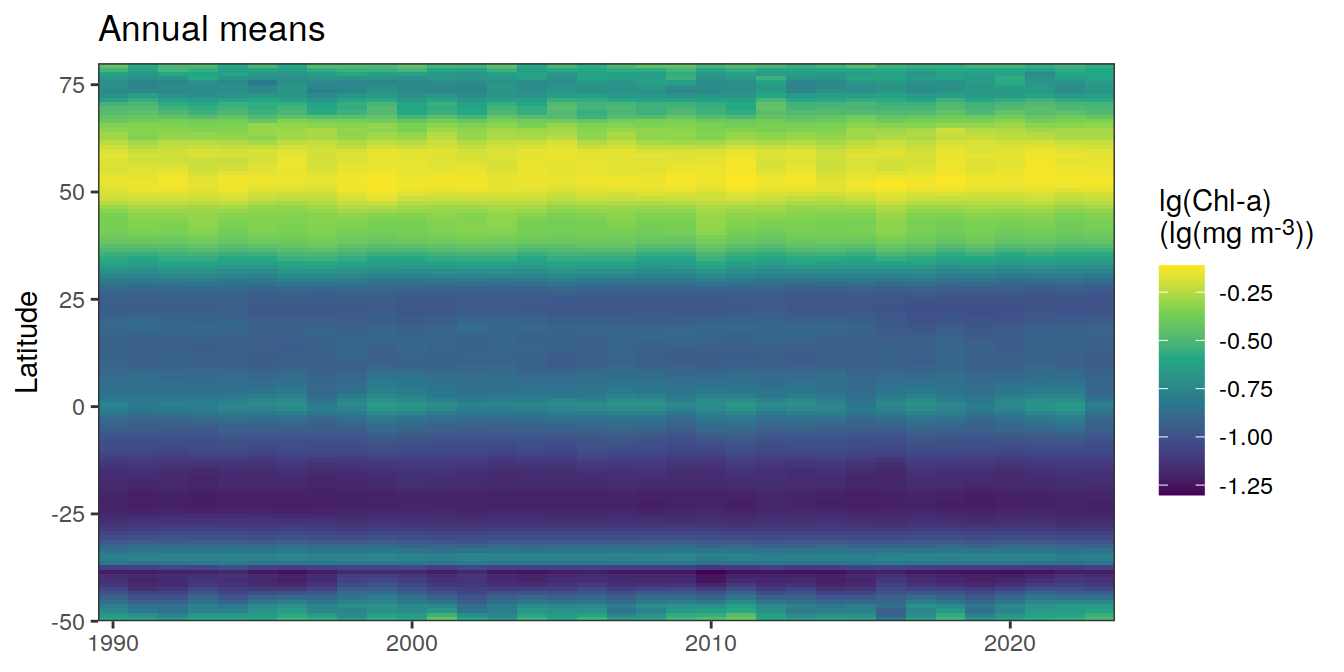
[[3]]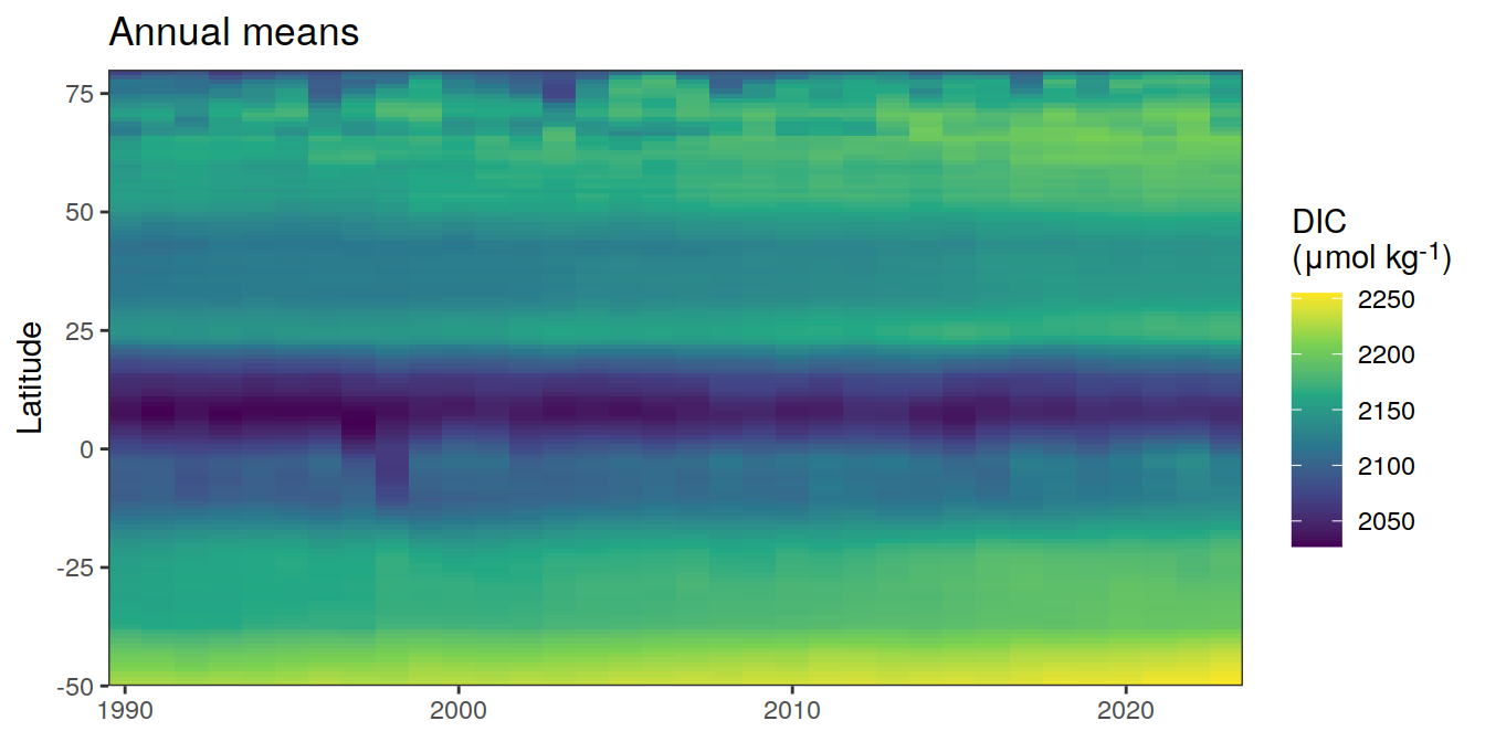
[[4]]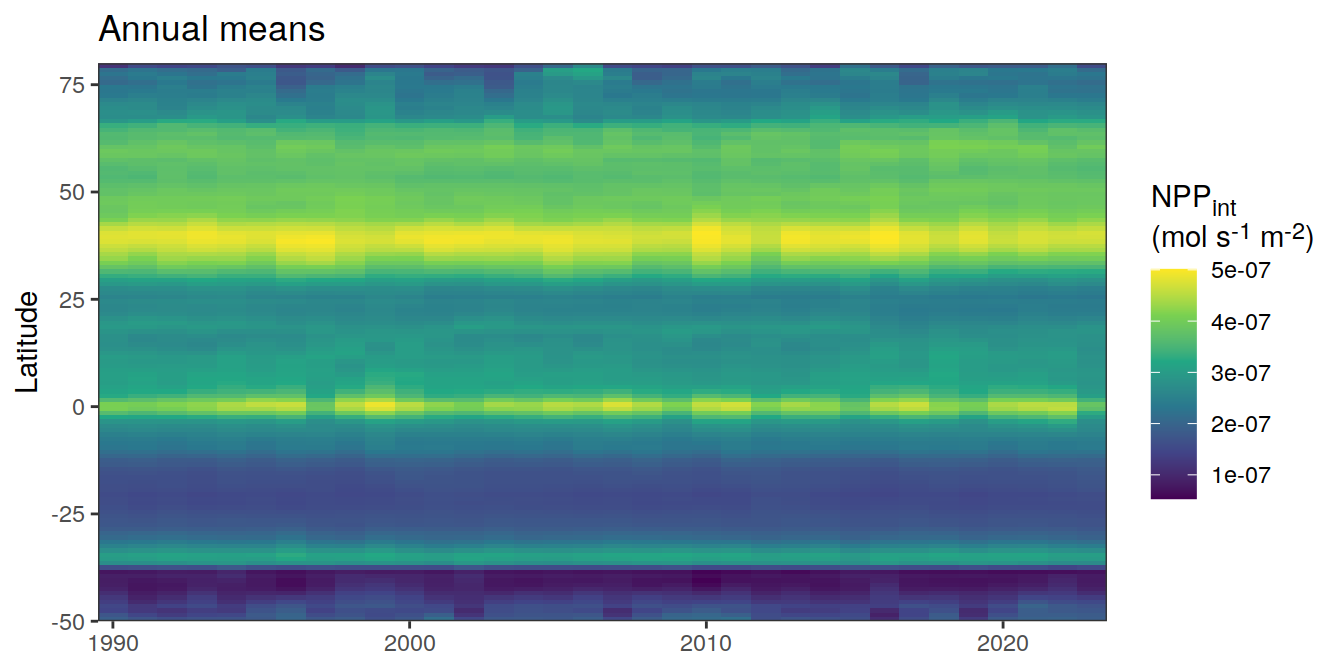
[[5]]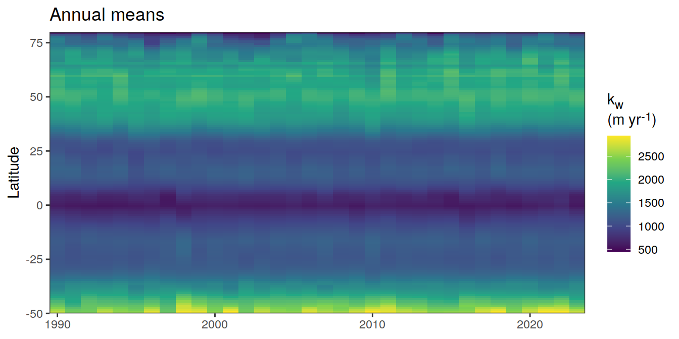
[[6]]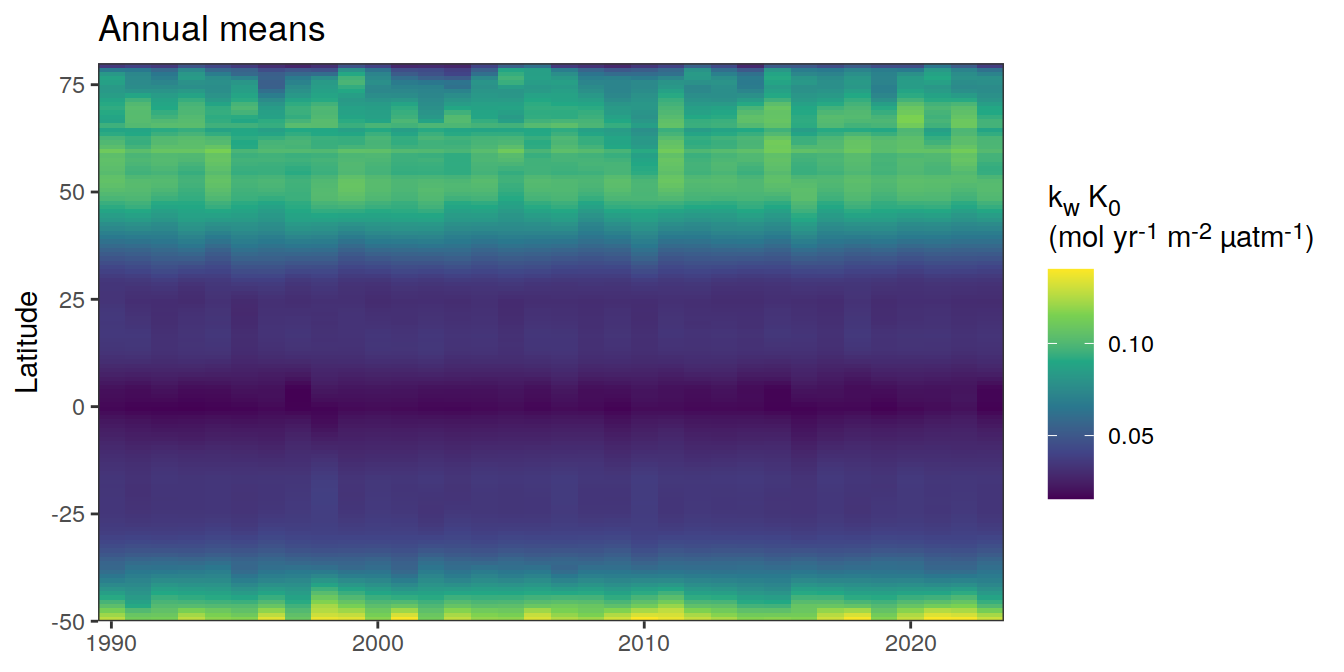
[[7]]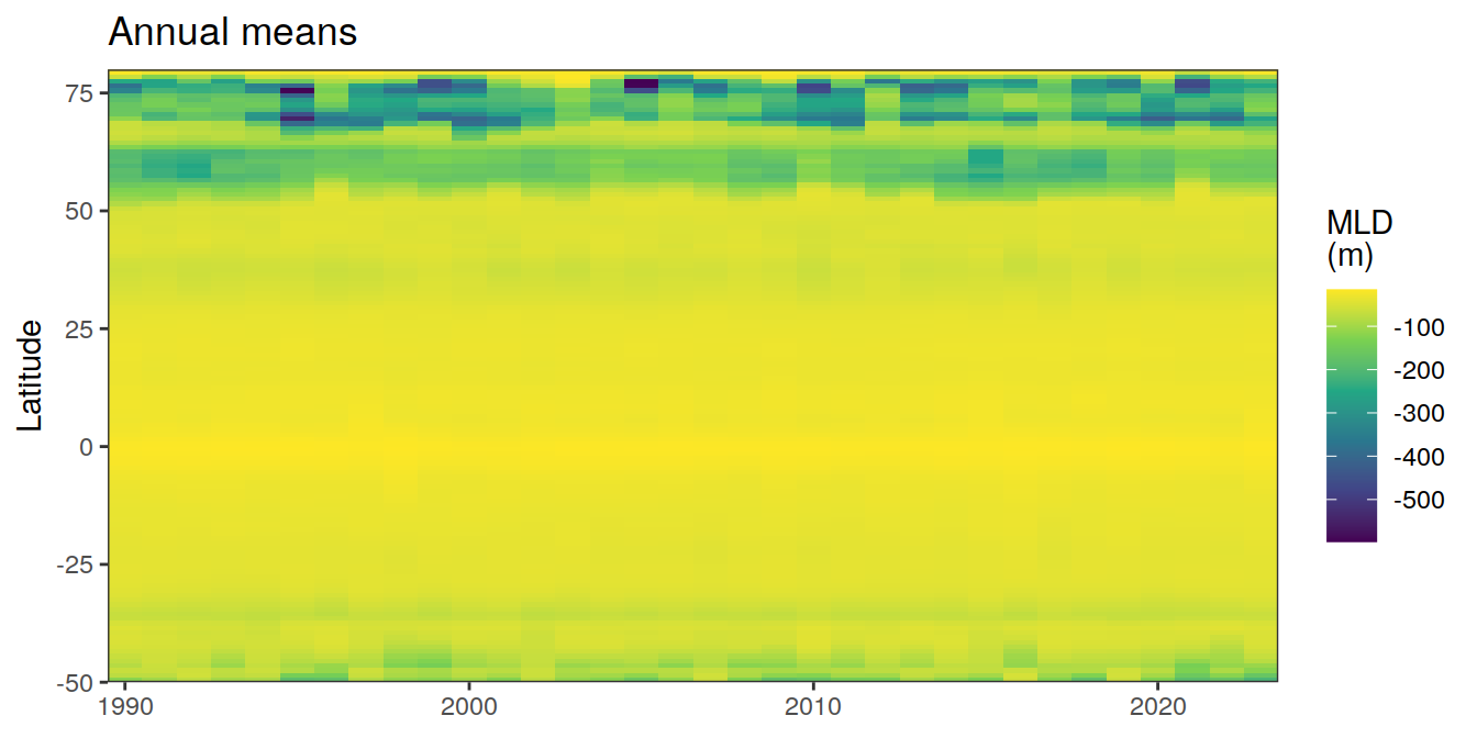
[[8]]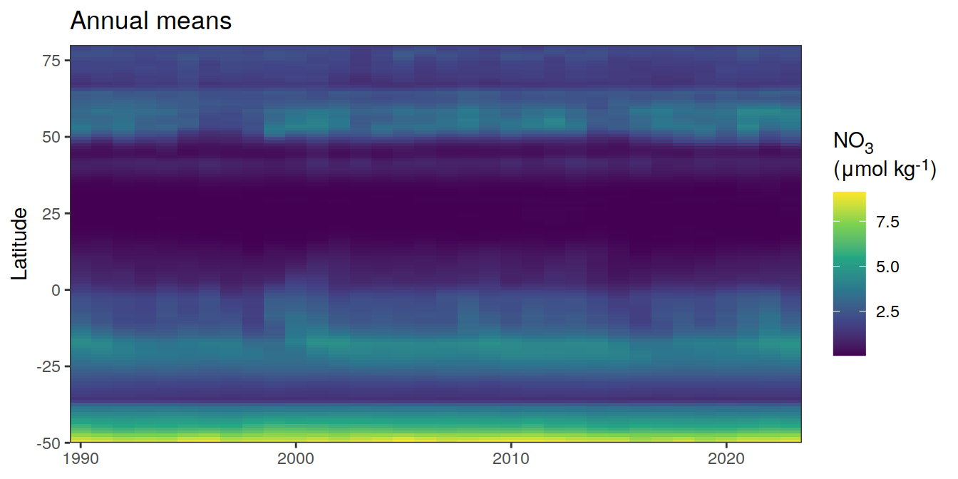
[[9]]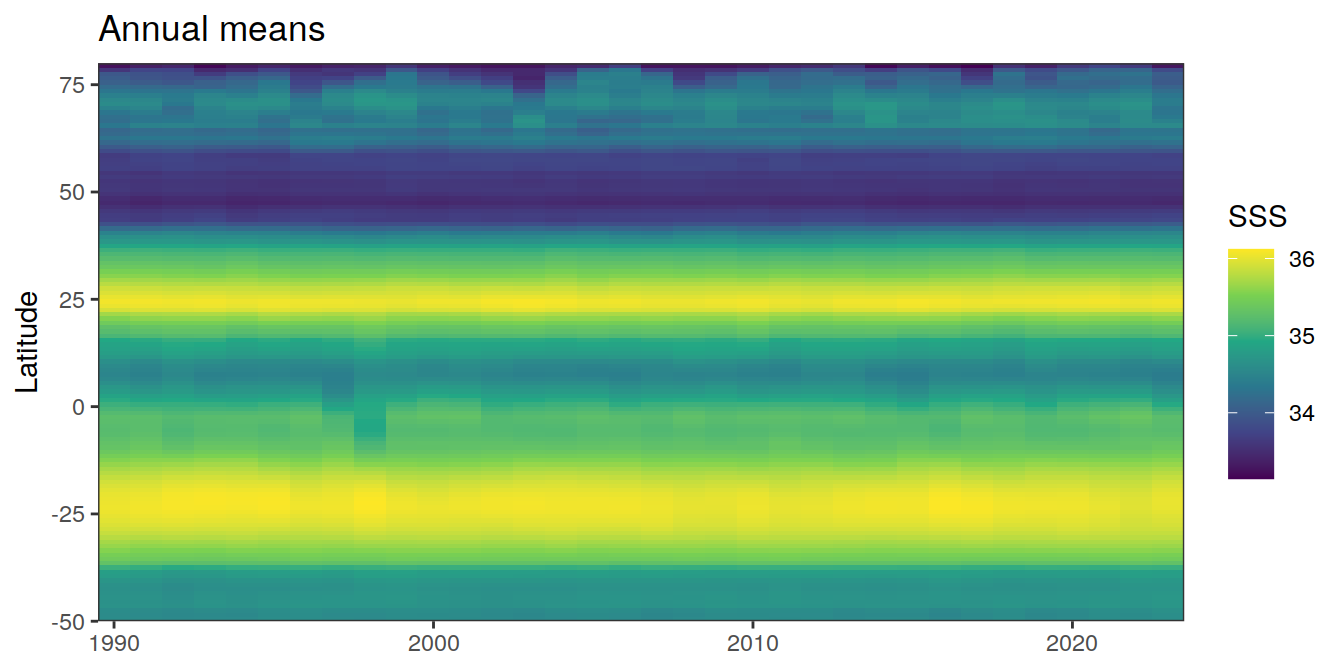
[[10]]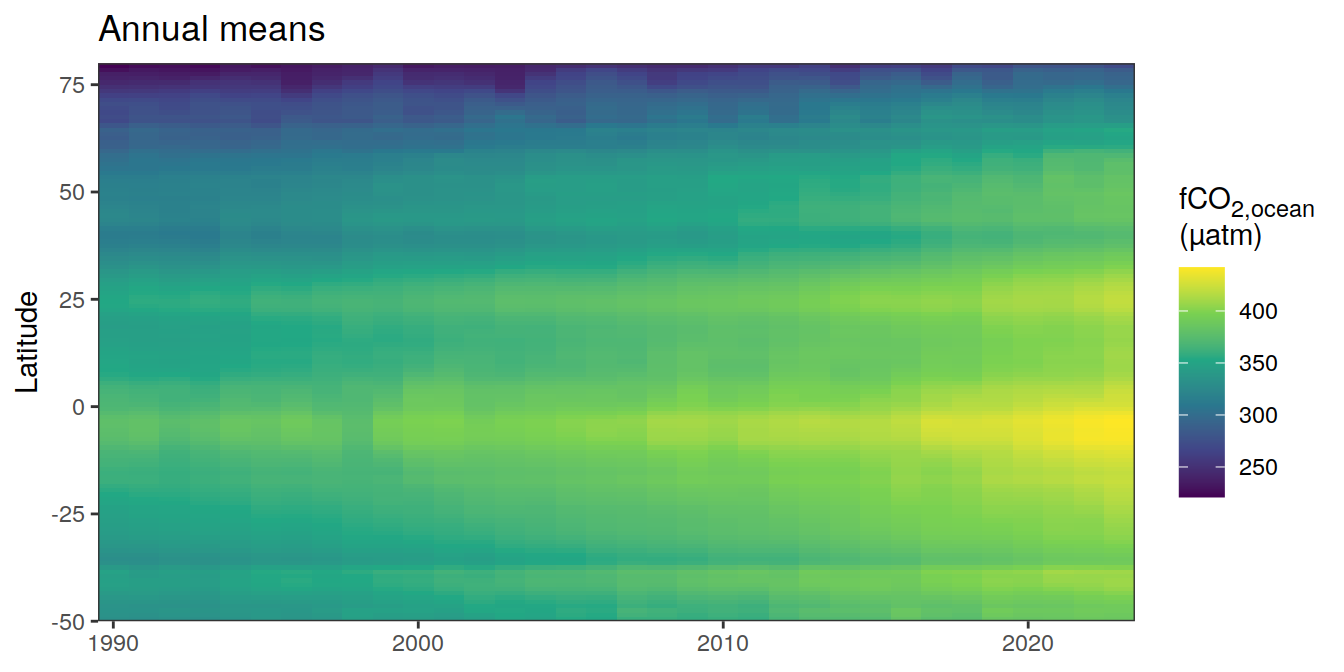
[[11]]
[[12]]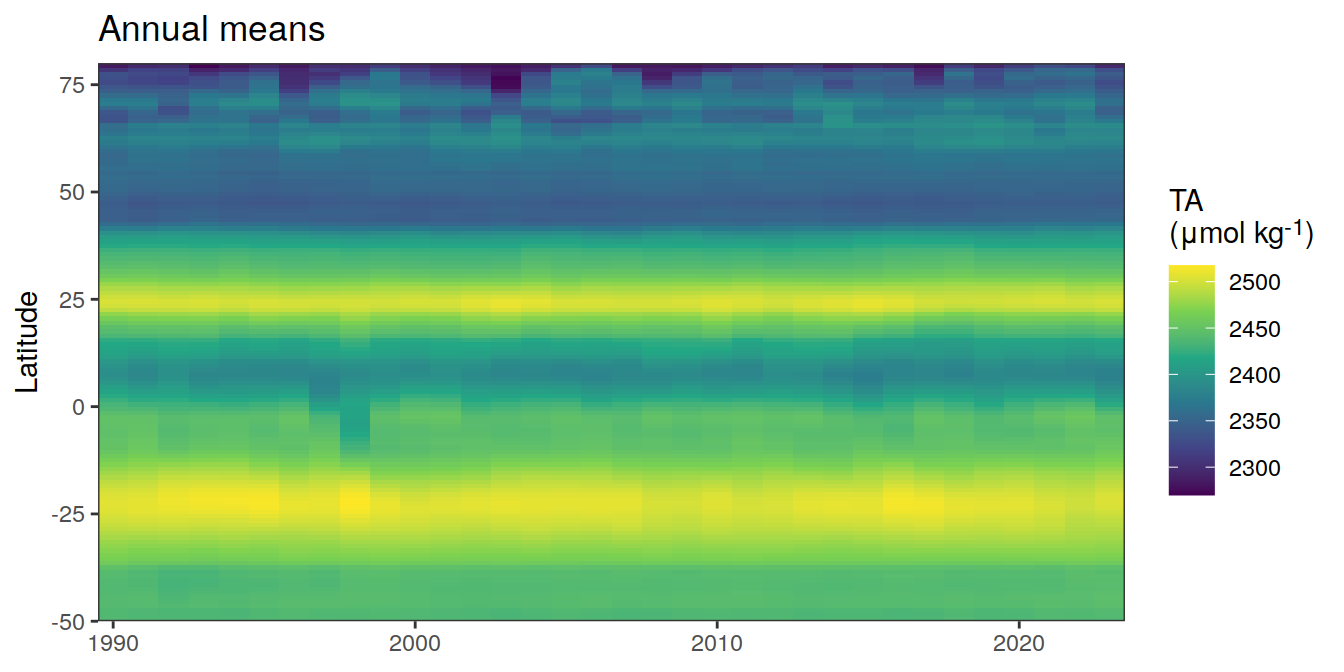
[[13]]
pco2_product_hovmoeller_monthly_annual %>%
  filter(name %in% name_divergent) %>%
  group_split(name) %>%
  # head(1) %>%
  map(
    ~ ggplot(data = .x,
             aes(year, lat, fill = value)) +
      geom_raster() +
      scale_fill_divergent(name = labels_breaks(.x %>% distinct(name))) +
      theme(legend.title = element_markdown()) +
      coord_cartesian(expand = 0) +
      labs(title = "Annual means",
           y = "Latitude") +
      theme(axis.title.x = element_blank())
  )
[[1]]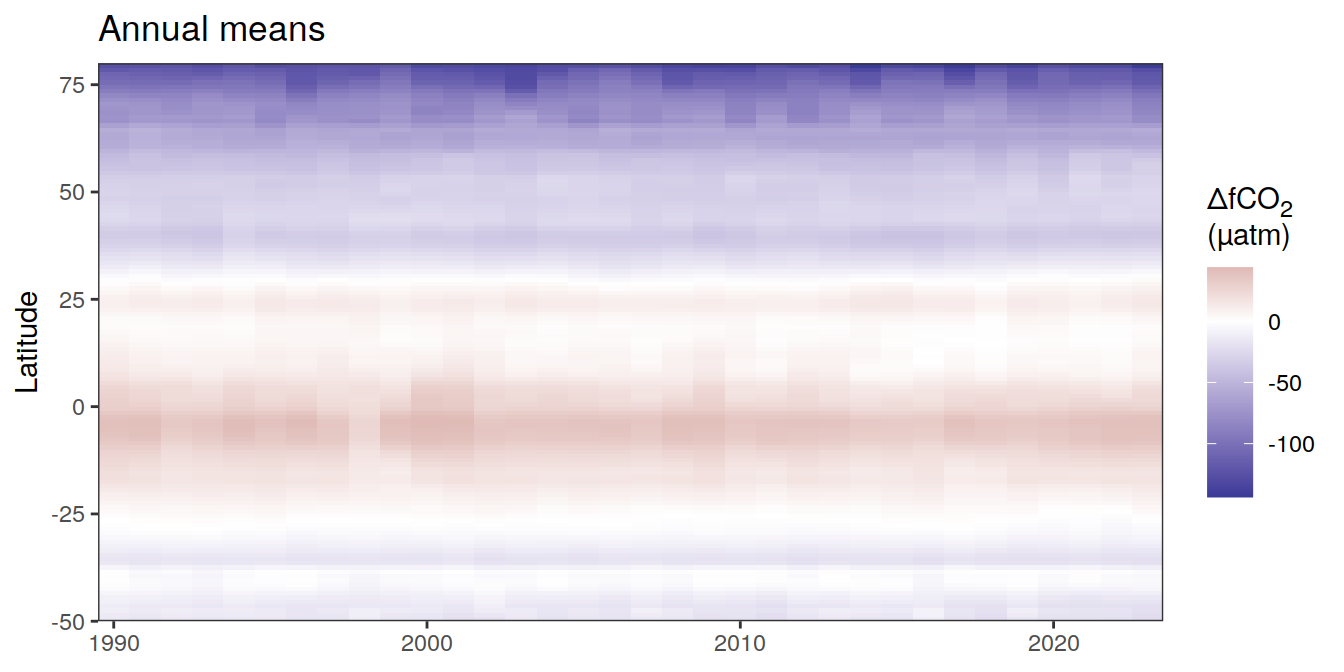
| Version | Author | Date |
|---|---|---|
| 054921b | jens-daniel-mueller | 2024-05-23 |
[[2]]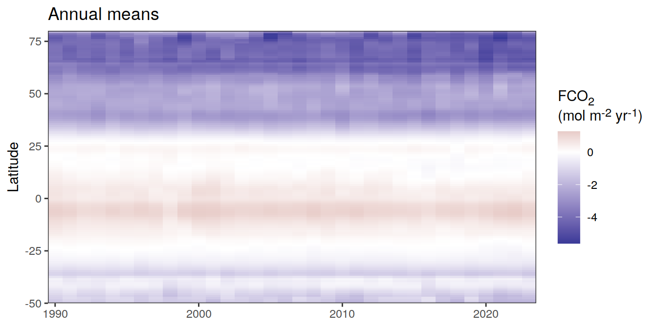
| Version | Author | Date |
|---|---|---|
| 054921b | jens-daniel-mueller | 2024-05-23 |
[[3]]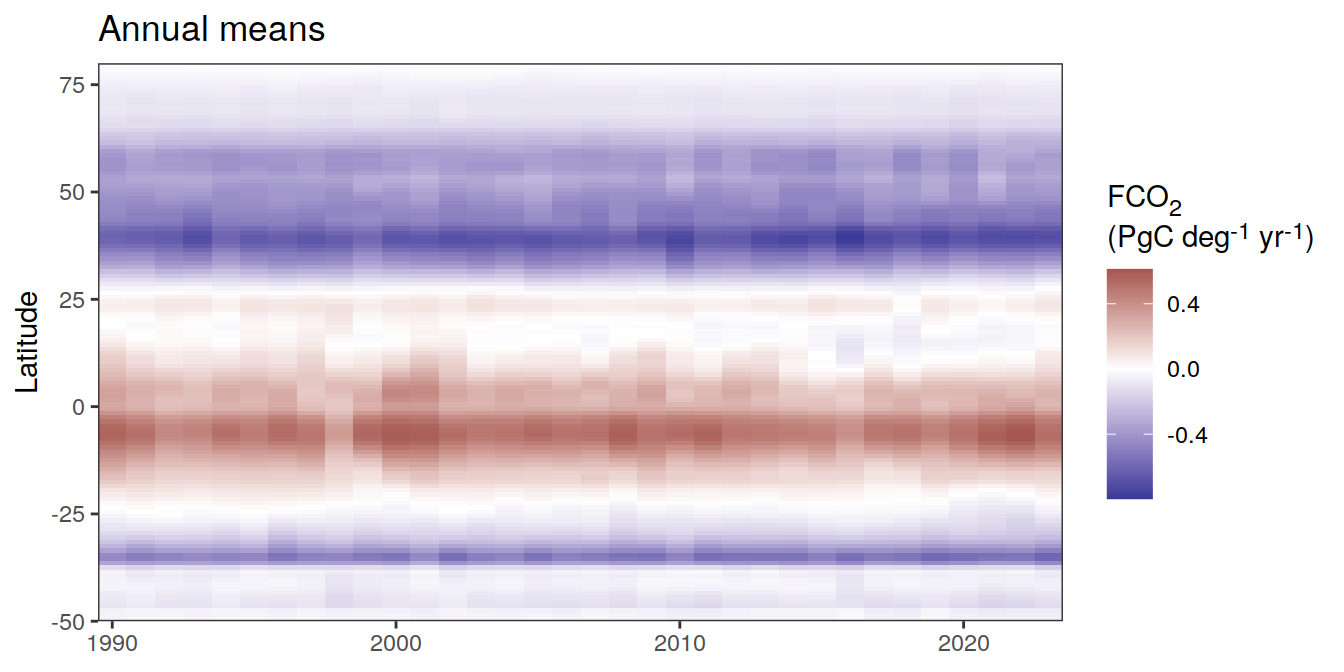
Monthly means
pco2_product_hovmoeller_monthly <-
  pco2_product %>%
  mutate(fgco2_int = fgco2) %>%
  select(-c(lon, time, biome)) %>%
  group_by(year, month, lat) %>%
  summarise(across(-c(fgco2_int, area),
                   ~ weighted.mean(., area, na.rm = TRUE)),
            across(fgco2_int,
                   ~ sum(. * area, na.rm = TRUE) * 12.01 * 1e-15)) %>%
  ungroup() %>%
  rename(fgco2_hov = fgco2_int) %>%
  filter(fgco2_hov != 0)


pco2_product_hovmoeller_monthly <-
  pco2_product_hovmoeller_monthly %>%
  pivot_longer(-c(year, month, lat)) %>%
  drop_na()

pco2_product_hovmoeller_monthly <-
  pco2_product_hovmoeller_monthly %>%
  mutate(decimal = year + (month-1) / 12)

pco2_product_hovmoeller_monthly %>%
  filter(!(name %in% name_divergent)) %>%
  group_split(name) %>%
  # head(1) %>%
  map(
    ~ ggplot(data = .x,
             aes(decimal, lat, fill = value)) +
      geom_raster() +
      scale_fill_viridis_c(name = labels_breaks(.x %>% distinct(name))) +
      theme(legend.title = element_markdown()) +
      labs(title = "Monthly means",
           y = "Latitude") +
      coord_cartesian(expand = 0) +
      theme(axis.title.x = element_blank())
  )
[[1]]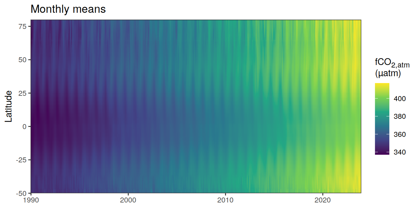
[[2]]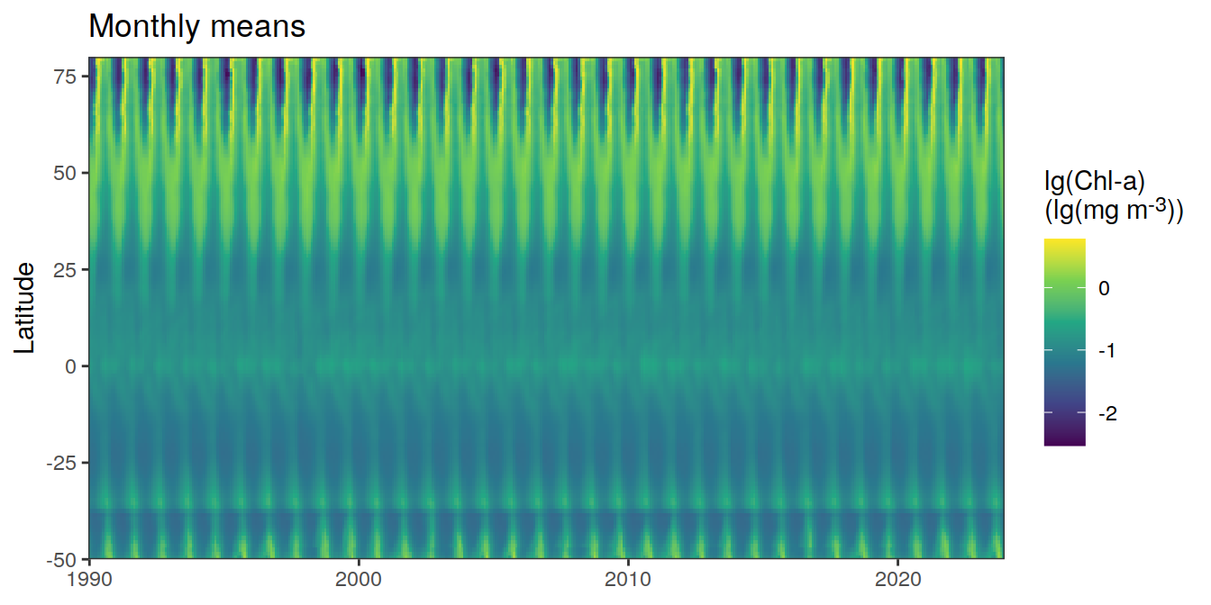
[[3]]
[[4]]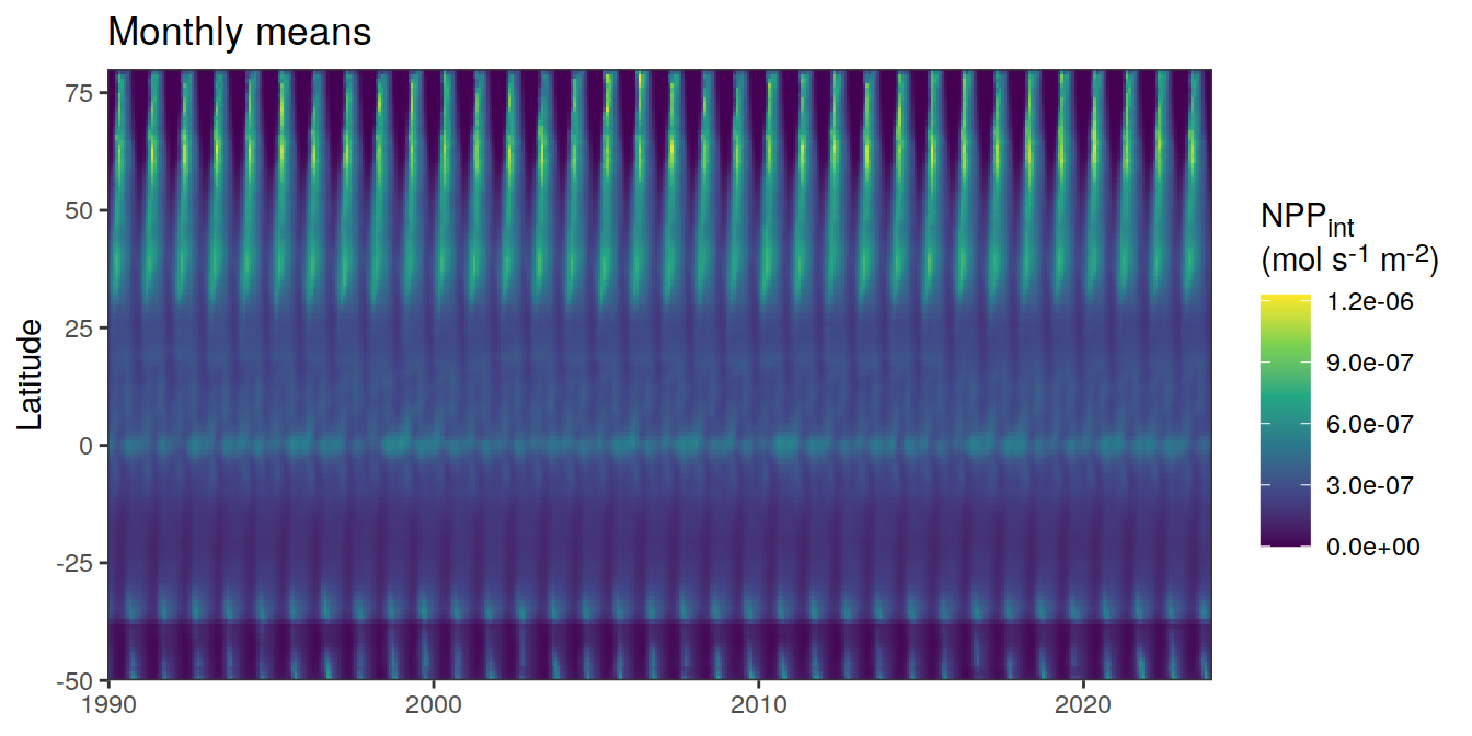
[[5]]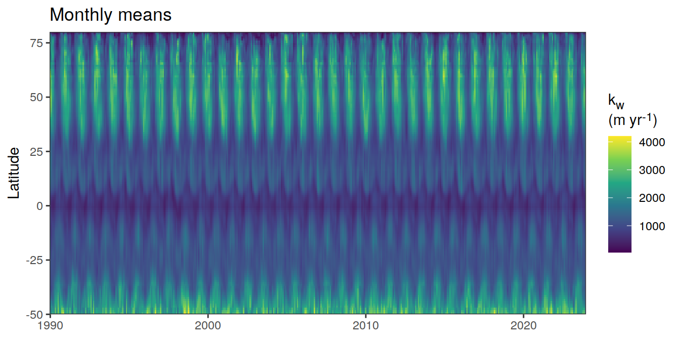
[[6]]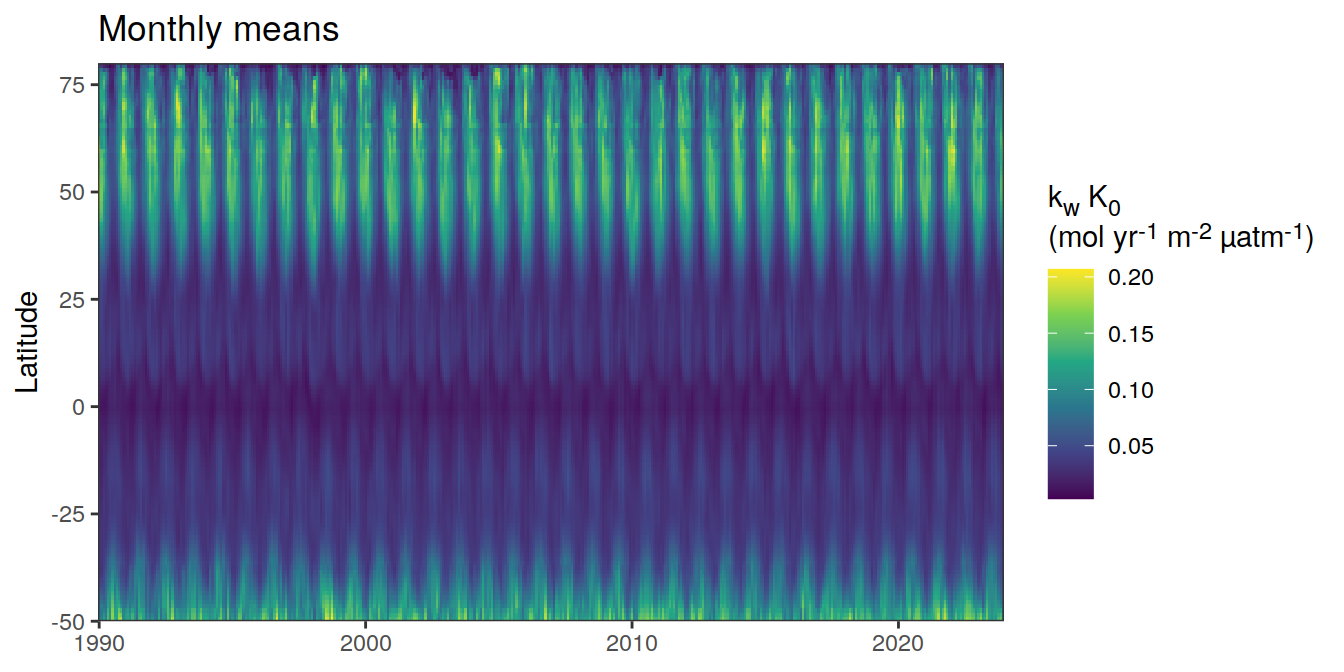
[[7]]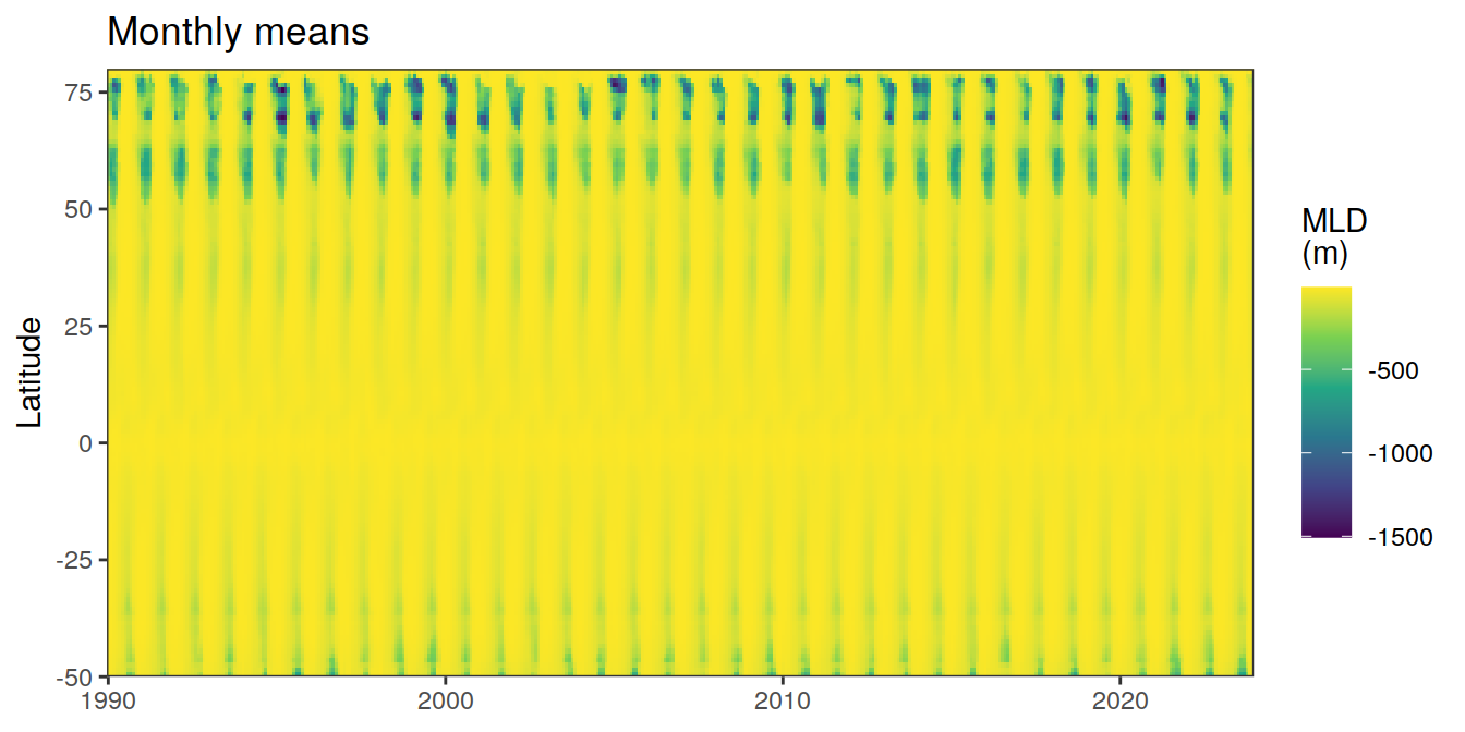
[[8]]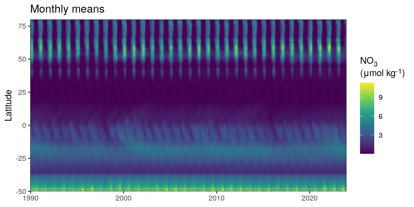
[[9]]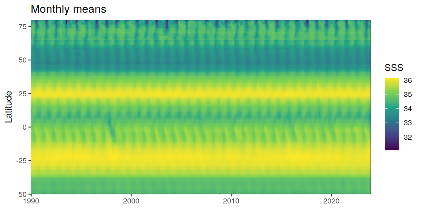
[[10]]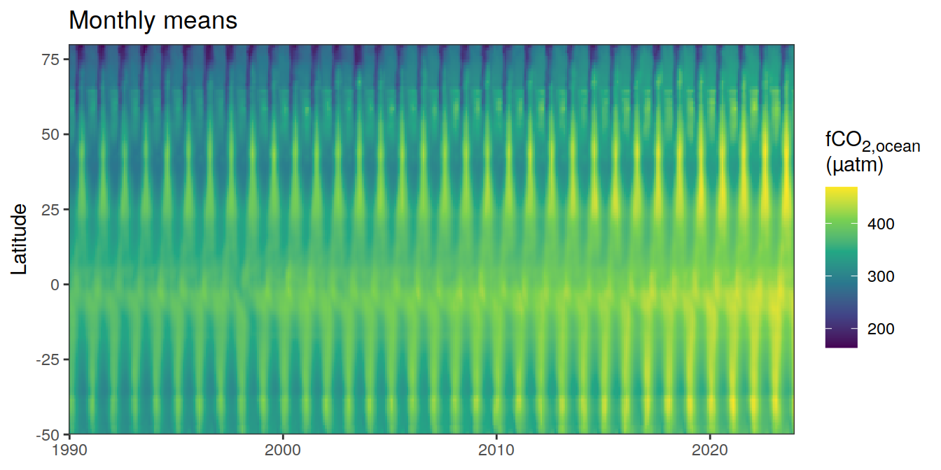
[[11]]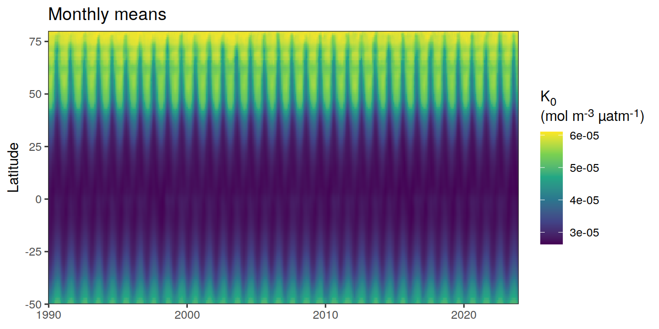
[[12]]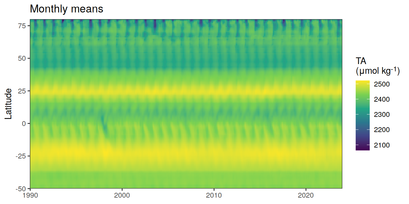
[[13]]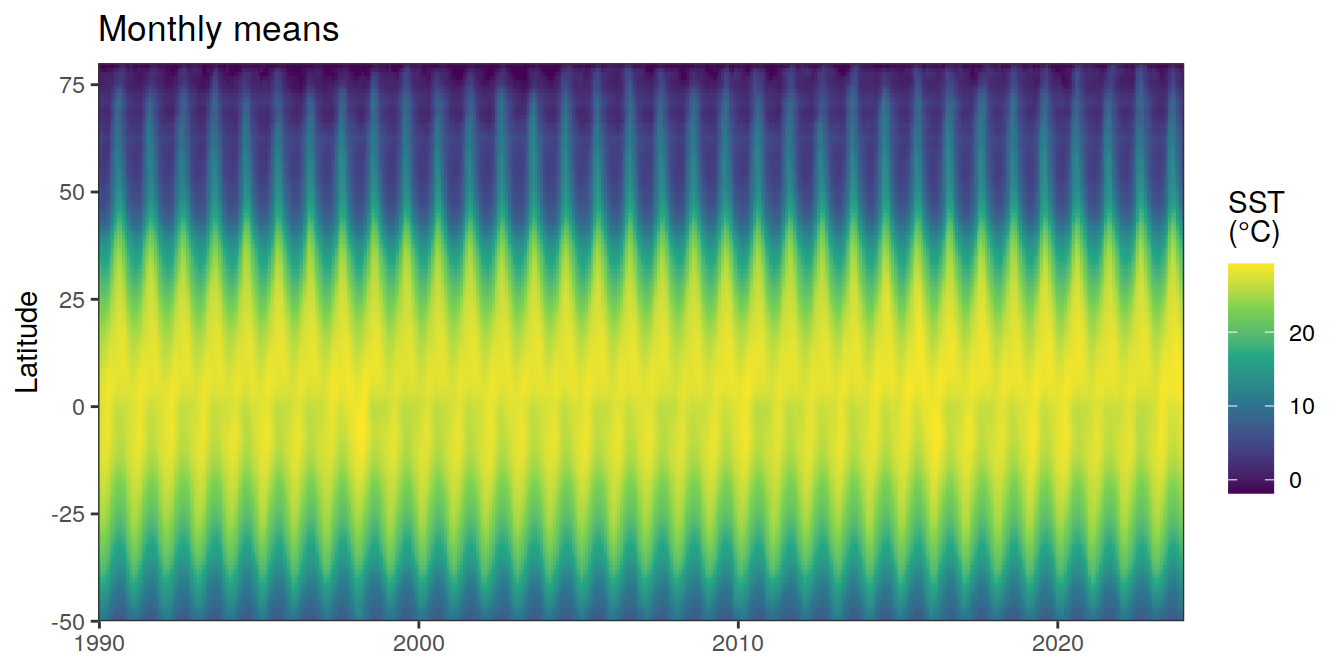
pco2_product_hovmoeller_monthly %>%
  filter(name %in% name_divergent) %>%
  group_split(name) %>%
  # head(1) %>%
  map(
    ~ ggplot(data = .x,
             aes(decimal, lat, fill = value)) +
      geom_raster() +
      scale_fill_divergent(name = labels_breaks(.x %>% distinct(name))) +
      theme(legend.title = element_markdown()) +
      labs(title = "Monthly means",
           y = "Latitude") +
      coord_cartesian(expand = 0) +
      theme(axis.title.x = element_blank())
  )
[[1]]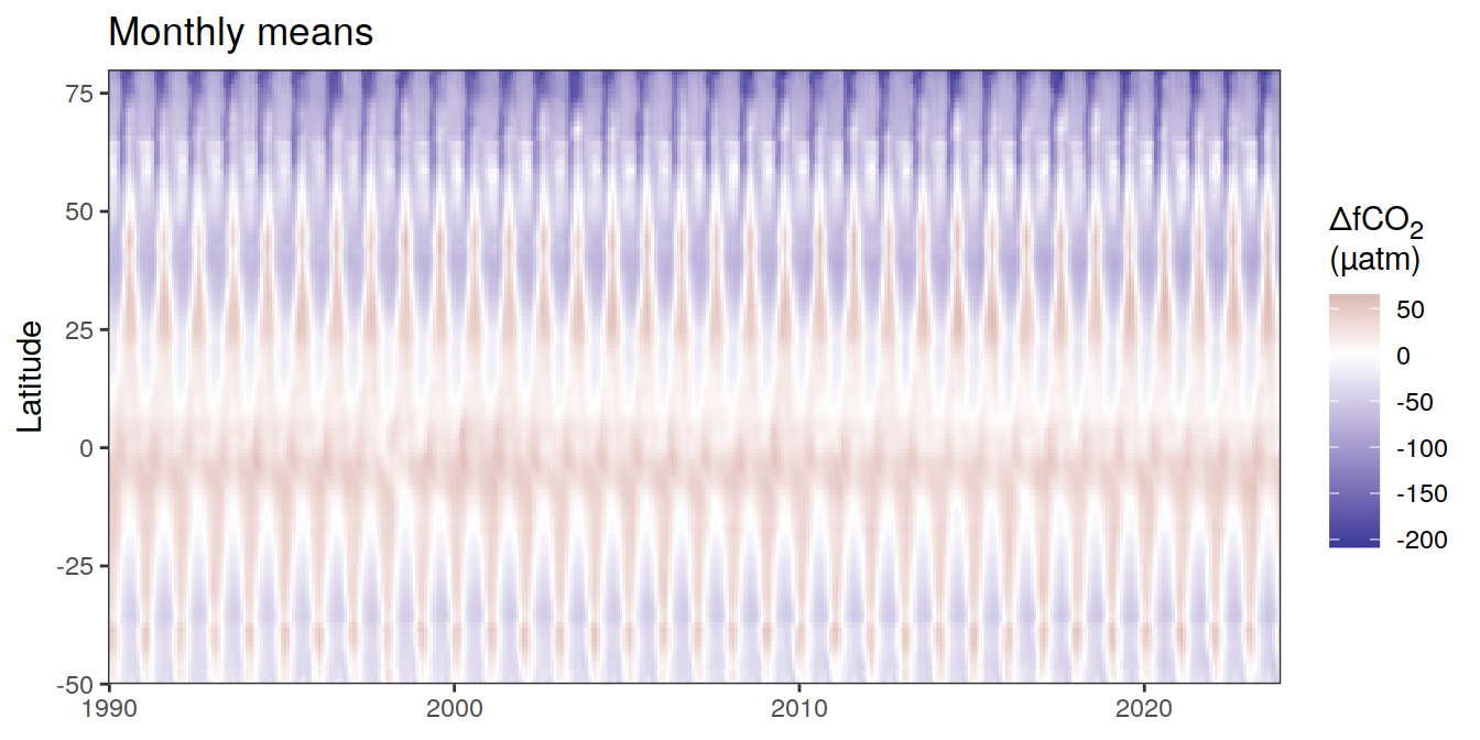
| Version | Author | Date |
|---|---|---|
| 054921b | jens-daniel-mueller | 2024-05-23 |
[[2]]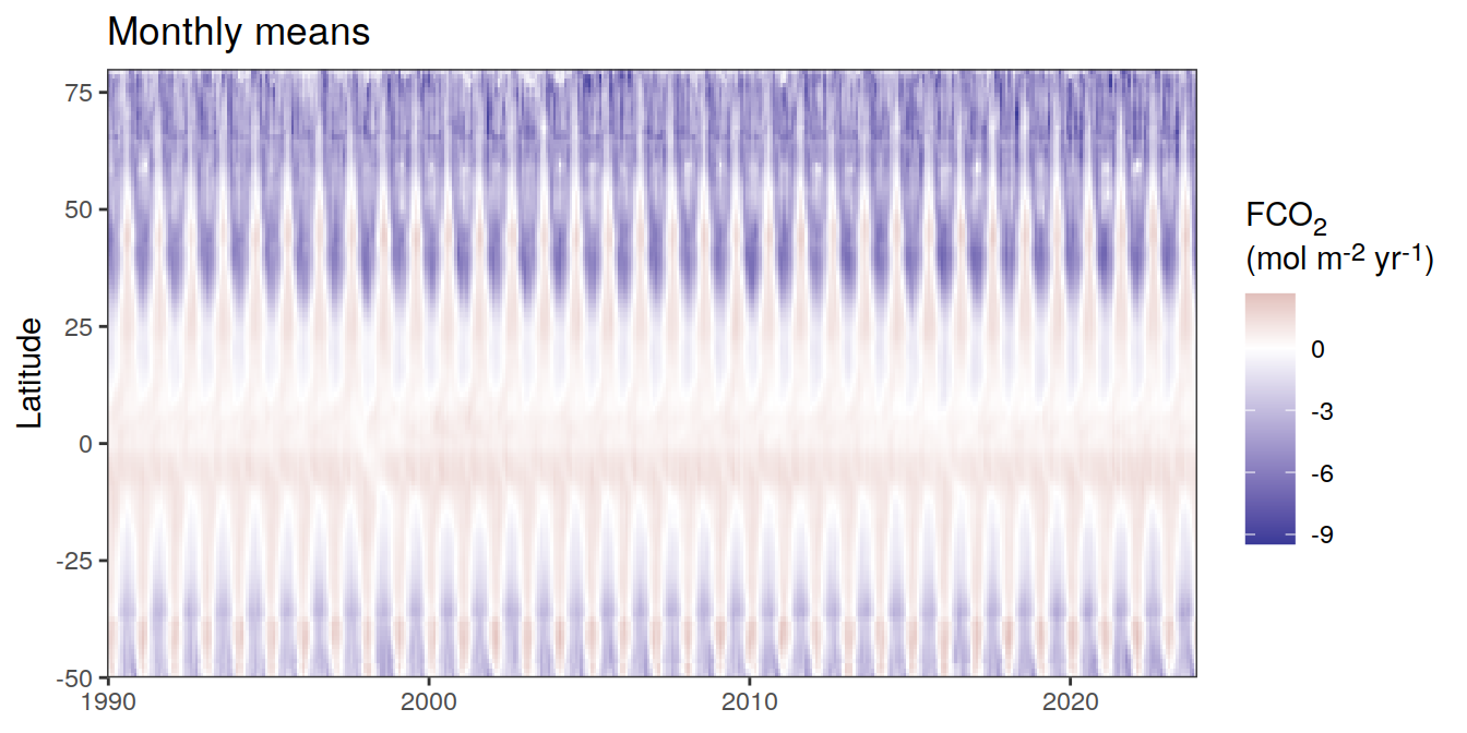
| Version | Author | Date |
|---|---|---|
| 054921b | jens-daniel-mueller | 2024-05-23 |
[[3]]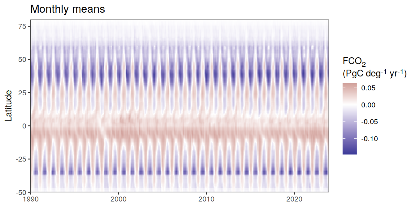
pCO2productanalysis_2023 <-
  knitr::knit_expand(
    file = here::here("analysis/child/pCO2_product_analysis.Rmd"),
    product_name = "FESOM-REcoM",
    year_anom = 2023
  )
2023 anomalies
Detection
For the detection of anomalies at any point in time and space, we fit regression models and compare the fitted to the actual value.
We use linear regression models for all parameters, except for , which are approximated with quadratic fits.
The regression models are fitted to all data since , except 2023.
anomaly_determination <- function(df,...) {

  group_by <- quos(...)
  # group_by <- quos(region, lat, depth)
  # df <- pco2_product_coarse_annual

  # Linear regression models

  df_lm <-
    df %>%
    filter(year != 2023,
           !(name %in% name_quadratic_fit)) %>%
    nest(data = -c(name, !!!group_by)) %>%
    mutate(
      fit = map(data, ~ lm(value ~ year, data = .x)),
      tidied = map(fit, tidy),
      augmented = map(fit, augment)
    )


  df_lm_year_anom <-
    full_join(
      df_lm %>%
        unnest(tidied) %>%
        select(name, !!!group_by, term, estimate) %>%
        pivot_wider(names_from = term,
                    values_from = estimate) %>%
        mutate(fit = `(Intercept)` + year * 2023) %>%
        select(name, !!!group_by, fit) %>%
        mutate(year = 2023),
      df %>%
        filter(year == 2023,
               !(name %in% name_quadratic_fit))
    ) %>%
    mutate(resid = value - fit)


  df_lm <-
    bind_rows(
      df_lm %>%
        unnest(augmented) %>%
        select(name, !!!group_by, year, value, fit = .fitted, resid = .resid),
      df_lm_year_anom
    )

  rm(df_lm_year_anom)

  # Quadratic regression models

  if(any(df %>% distinct(name) %>% pull() %in% name_quadratic_fit)){

  df_quadratic <-
    df %>%
    filter(year != 2023,
           name %in% name_quadratic_fit) %>%
    nest(data = -c(name, !!!group_by)) %>%
    mutate(
      fit = map(data, ~ lm(value ~ year + I(year ^ 2), data = .x)),
      tidied = map(fit, tidy),
      augmented = map(fit, augment)
    )

  df_quadratic_year_anom <-
    full_join(
      df_quadratic %>%
        unnest(tidied) %>%
        select(name, !!!group_by, term, estimate) %>%
        pivot_wider(names_from = term,
                    values_from = estimate) %>%
        mutate(fit = `(Intercept)` + year * 2023 + `I(year^2)` * 2023 ^ 2) %>%
        select(name, !!!group_by, fit) %>%
        mutate(year = 2023),
      df %>%
        filter(year == 2023,
               name %in% name_quadratic_fit)
    ) %>%
    mutate(resid = value - fit)


  df_quadratic <-
    bind_rows(
      df_quadratic %>%
        unnest(augmented) %>%
        select(name, !!!group_by, year, value, fit = .fitted, resid = .resid),
      df_quadratic_year_anom
    )

  rm(df_quadratic_year_anom)

  # Join linear and quadratic regression results

  df_regression <-
    bind_rows(df_lm,
              df_quadratic)

  rm(df_lm,
     df_quadratic)

  } else{

    df_regression <- df_lm

    rm(df_lm)
  }

  df_regression <-
    df_regression %>%
    arrange(year)


  return(df_regression)

}
anomaly_determination <- function(df,...) {
group_by <- quos(...)
# group_by <- quos(biome)
# group_by <- quos(lon, lat)
# df <- pco2_product_coarse_annual
# Climatoligcal mean
df_mean <-
df %>%
filter(year < 2023,
year >= 2023-5) %>%
group_by(name, !!!group_by) %>%
summarize(
fit = mean(value, na.rm = TRUE)
) %>%
ungroup()
df_mean <-
full_join(
df_mean,
df
) %>%
mutate(resid = value - fit)
return(df_mean)
}Maps
The following maps show the absolute state of each variable in 2023 as provided through the pCO2 product, the change in that variable from 1990 to 2023, as well es the anomalies in 2023. Changes and anomalies are determined based on the predicted value of a linear regression model fit to the data from 1990 to 2022.
Maps are first presented as annual means, and than as monthly means. Note that the 2023 predictions for the monthly maps are done individually for each month, such the mean seasonal anomaly from the annual mean is removed.
Note: The increase the computational speed, I regridded all maps to 5X5° grid.
Annual means
2023 absolute
pco2_product_coarse_annual_regression <-
  pco2_product_coarse_annual %>%
  drop_na() %>%
  anomaly_determination(lon, lat)

pco2_product_coarse_annual_regression <-
  pco2_product_coarse_annual_regression %>%
  drop_na()

pco2_product_coarse_annual_regression %>%
  filter(year == 2023,
         !(name %in% name_divergent)) %>%
  group_split(name) %>%
  # head(1) %>%
  map(
    ~ map +
      geom_tile(data = .x,
                aes(lon, lat, fill = value)) +
      labs(title = paste("Annual mean", 2023)) +
      scale_fill_viridis_c(name = labels_breaks(.x %>% distinct(name))) +
      theme(legend.title = element_markdown())
  )
[[1]]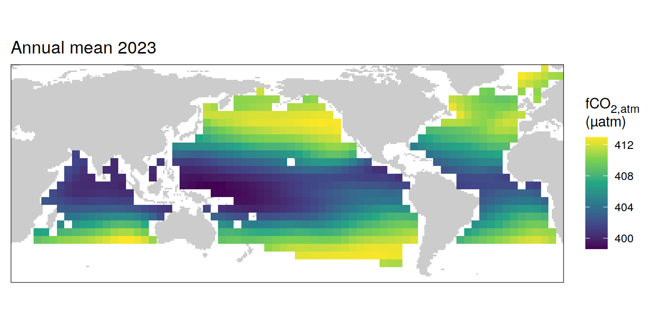
[[2]]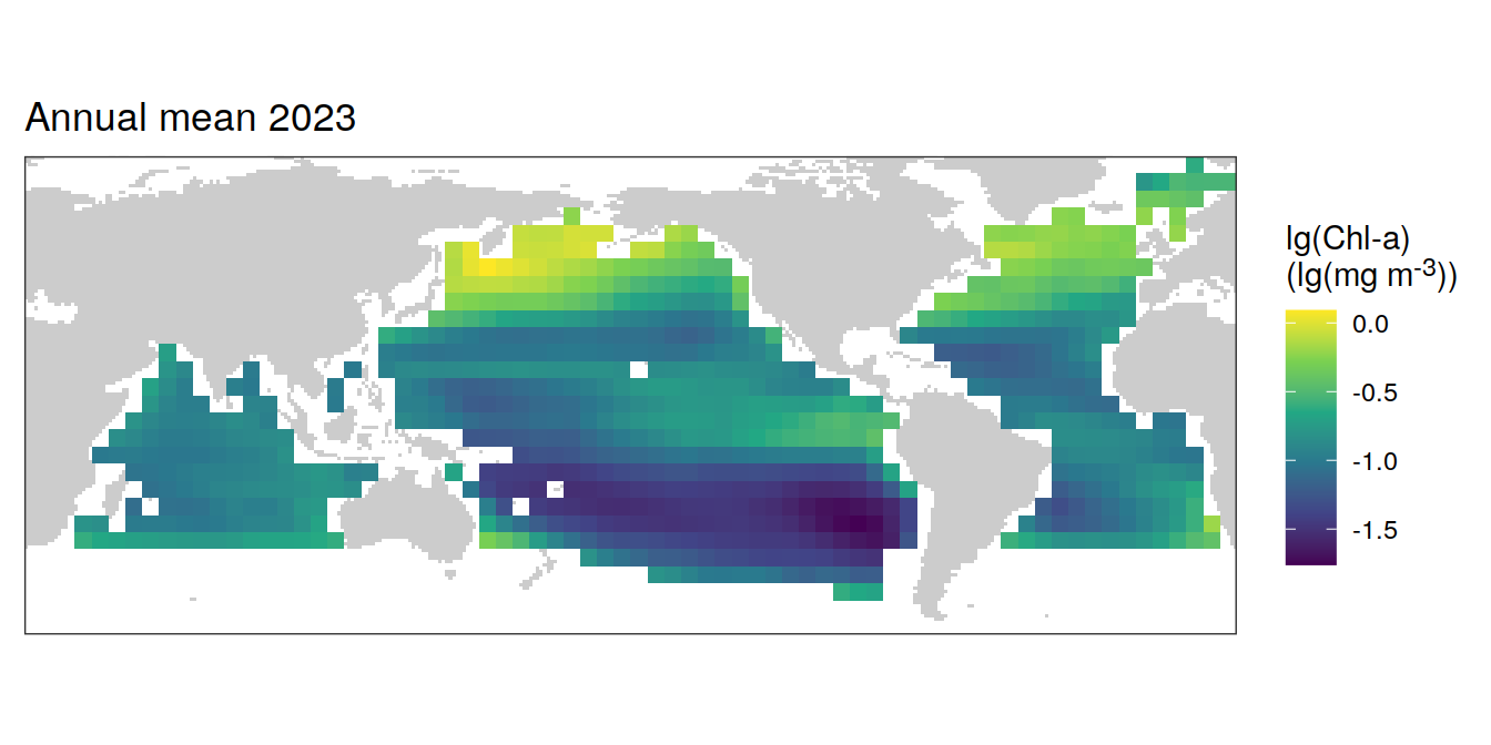
[[3]]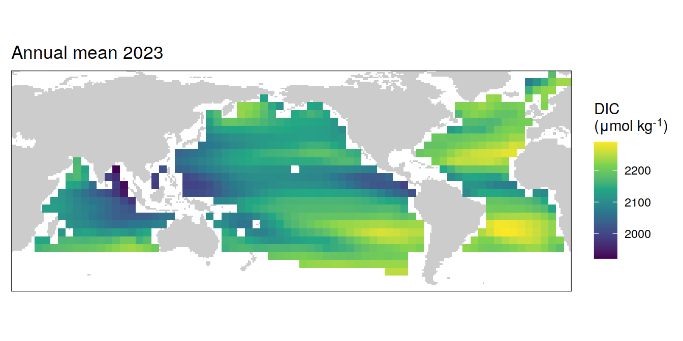
[[4]]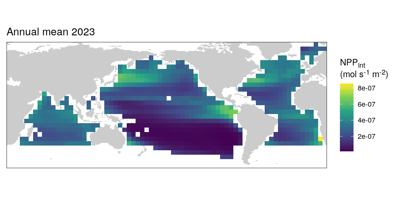
[[5]]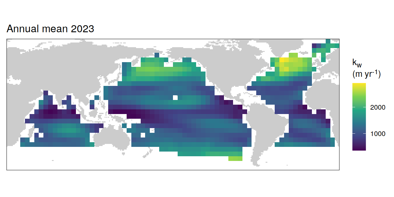
[[6]]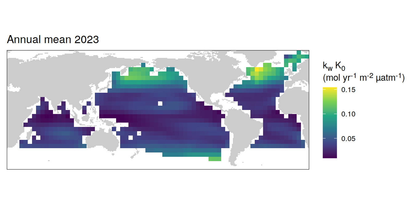
[[7]]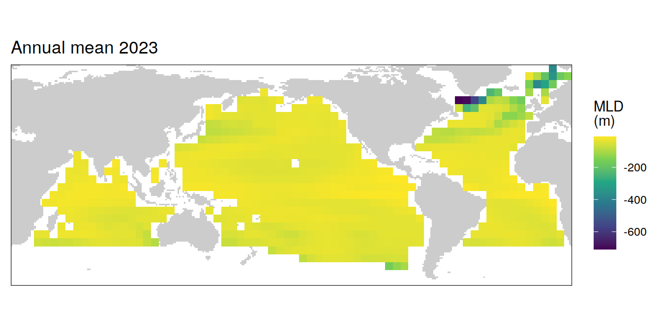
[[8]]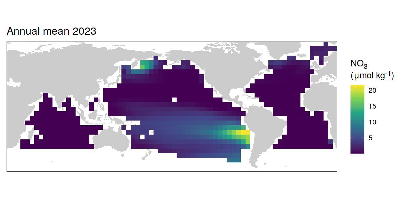
[[9]]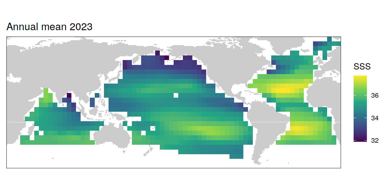
[[10]]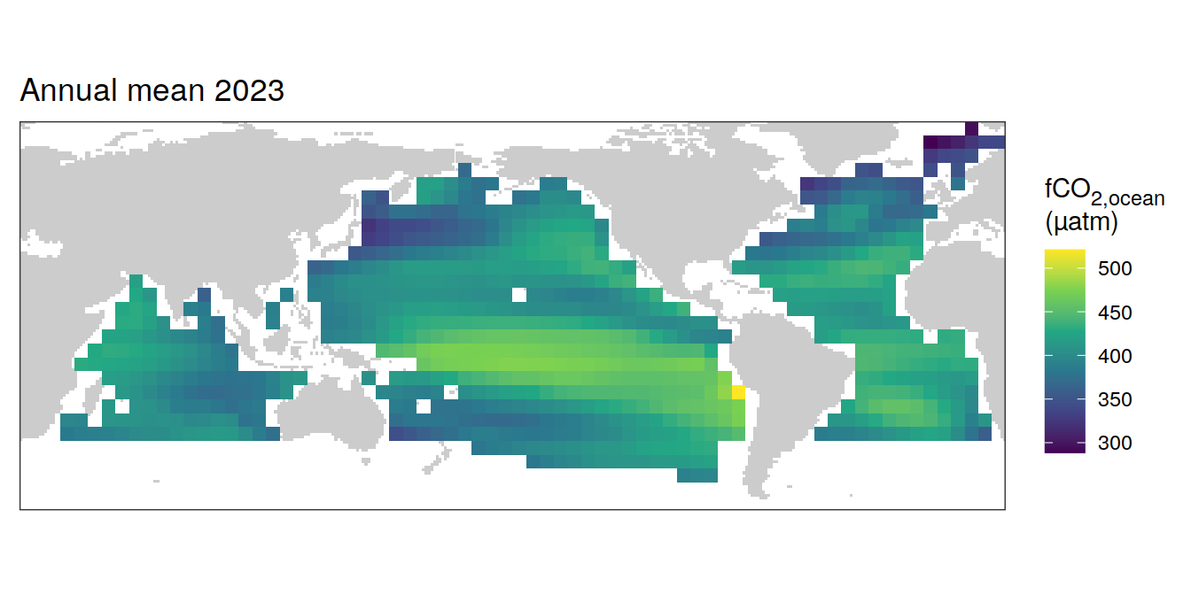
[[11]]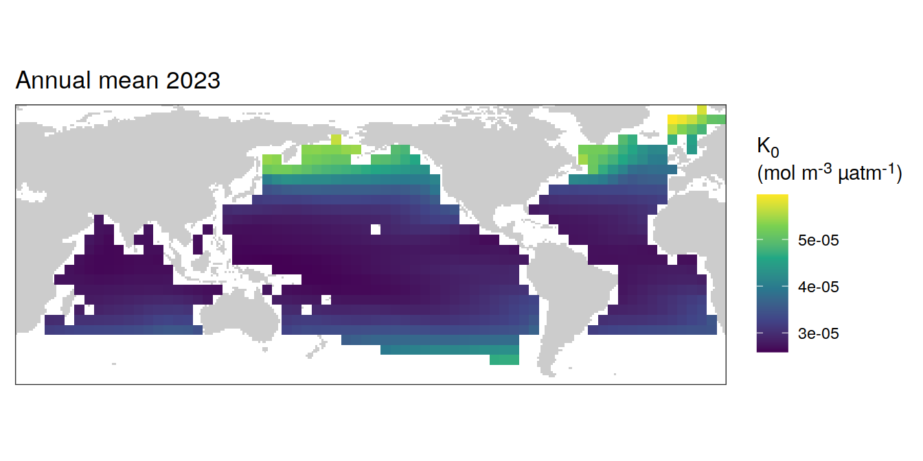
[[12]]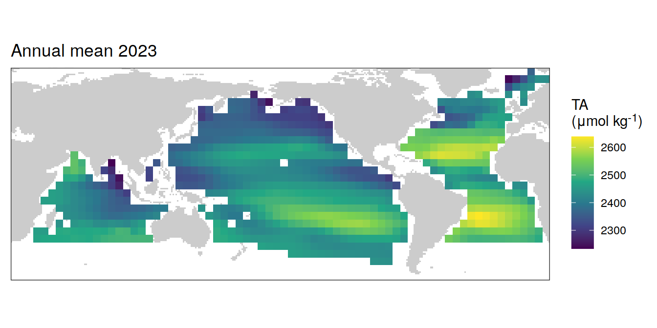
[[13]]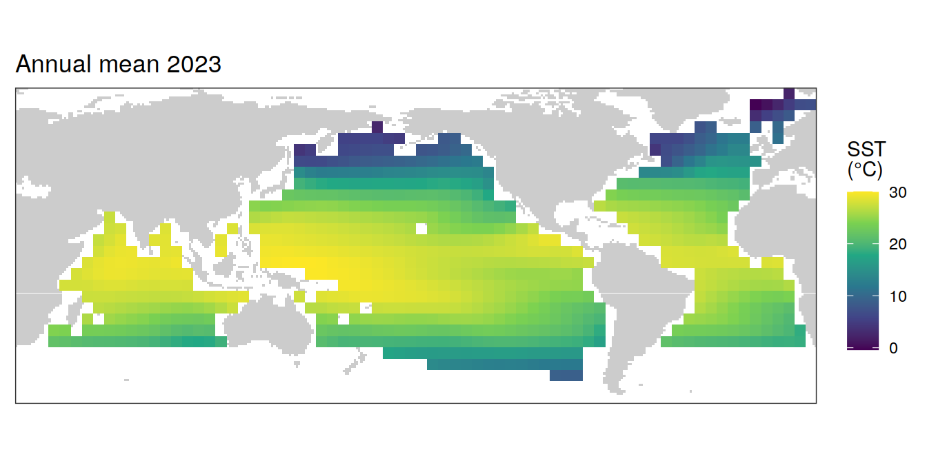
| Version | Author | Date |
|---|---|---|
| 054921b | jens-daniel-mueller | 2024-05-23 |
pco2_product_coarse_annual_regression %>%
  filter(year == 2023,
         name %in% name_divergent) %>%
  group_split(name) %>%
  # head(1) %>%
  map( ~ map +
         geom_tile(data = .x,
                   aes(lon, lat, fill = value)) +
         labs(title = paste("Annual mean", 2023)) +
         scale_fill_divergent(
           name = labels_breaks(.x %>% distinct(name))) +
         theme(legend.title = element_markdown())
  )
[[1]]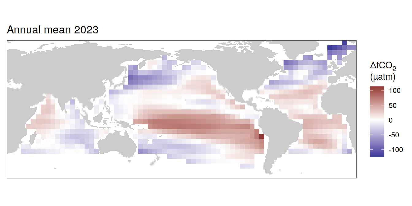
| Version | Author | Date |
|---|---|---|
| 054921b | jens-daniel-mueller | 2024-05-23 |
[[2]]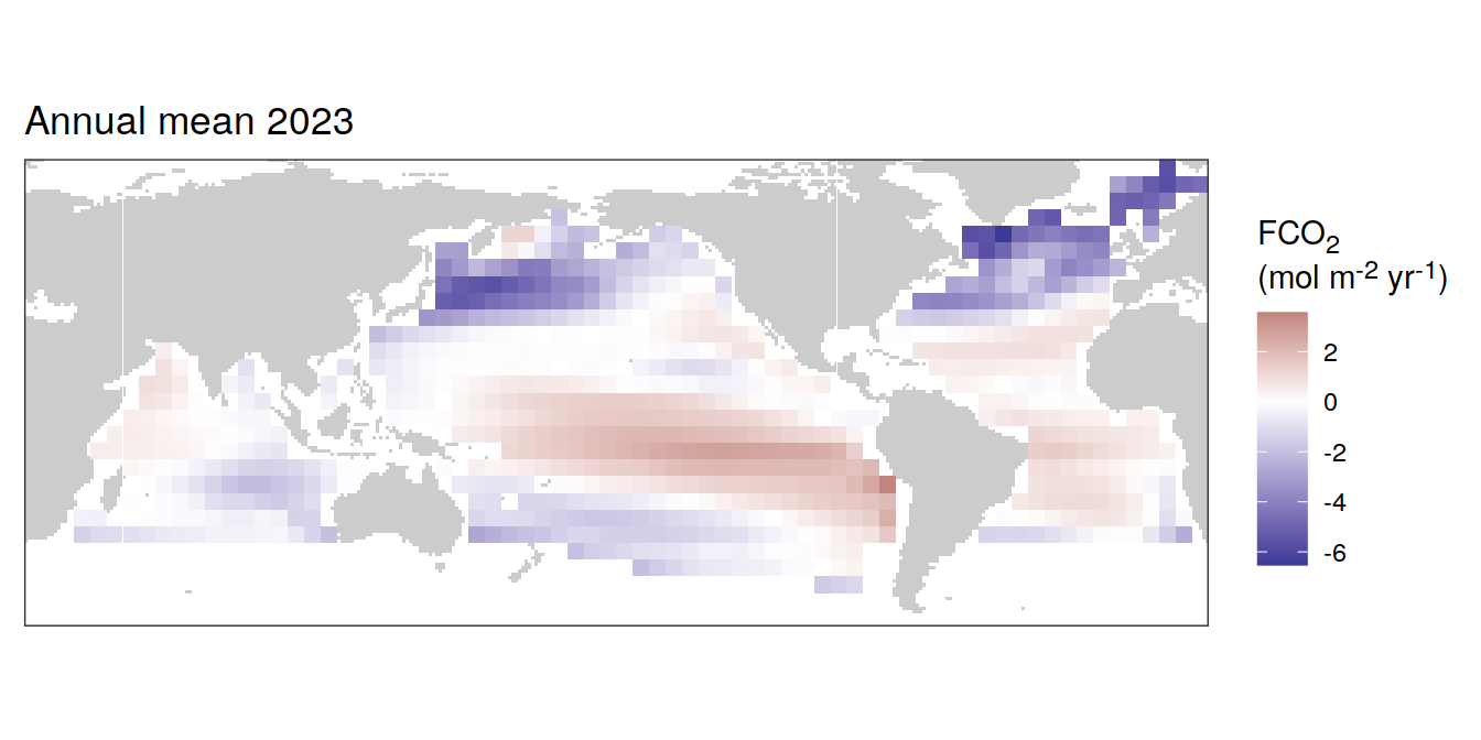
Trends
pco2_product_coarse_annual_regression <-
  pco2_product_coarse_annual_regression %>%
  group_by(name) %>%
  filter(year %in% c(min(year), max(year), 2023)) %>%
  ungroup()

pco2_product_coarse_annual_regression %>%
  select(-c(value, resid)) %>%
  filter(year %in% c(min(year), max(year))) %>%
  arrange(year) %>%
  group_by(lon, lat, name) %>%
  mutate(change = fit - lag(fit),
         period = paste(lag(year), year, sep = "-")) %>%
  ungroup() %>%
  filter(!is.na(change)) %>%
  group_split(name) %>%
  # head(1) %>%
  map(
    ~ map +
      geom_tile(data = .x,
                aes(lon, lat, fill = change)) +
      labs(title =  paste("Change: ",.x$period)) +
      scale_fill_divergent(name = labels_breaks(.x %>% distinct(name))) +
      theme(legend.title = element_markdown())
  )
[[1]]
[[2]]
[[3]]
[[4]]
[[5]]
[[6]]
[[7]]
[[8]]
[[9]]
[[10]]
[[11]]
[[12]]
[[13]]
| Version | Author | Date |
|---|---|---|
| 054921b | jens-daniel-mueller | 2024-05-23 |
[[14]]
| Version | Author | Date |
|---|---|---|
| 054921b | jens-daniel-mueller | 2024-05-23 |
[[15]]
2023 anomaly
pco2_product_coarse_annual_regression %>%
  filter(year == 2023) %>%
  group_split(name) %>%
  # head(1) %>%
  map( ~ map +
         geom_tile(data = .x,
                   aes(lon, lat, fill = resid)) +
         labs(title =  paste(2023,"anomaly")) +
         scale_fill_divergent(
           name = labels_breaks(.x %>% distinct(name))) +
         theme(legend.title = element_markdown())
  )
[[1]]
[[2]]
[[3]]
[[4]]
[[5]]
[[6]]
[[7]]
[[8]]
[[9]]
[[10]]
[[11]]
[[12]]
[[13]]
| Version | Author | Date |
|---|---|---|
| 054921b | jens-daniel-mueller | 2024-05-23 |
[[14]]
| Version | Author | Date |
|---|---|---|
| 054921b | jens-daniel-mueller | 2024-05-23 |
[[15]]
pco2_product_coarse_annual_regression %>%
  write_csv(paste0("../data/","FESOM-REcoM","_","2023","_anomaly_map_annual.csv"))
Monthly means
2023 absolute
pco2_product_coarse_monthly_regression <-
  pco2_product_coarse_monthly %>%
  drop_na() %>%
  anomaly_determination(lon, lat, month)

pco2_product_coarse_monthly_regression <-
  pco2_product_coarse_monthly_regression %>%
  drop_na()


pco2_product_coarse_monthly_regression %>%
  filter(year == 2023,
         !(name %in% name_divergent)) %>%
  group_split(name) %>%
  # head(1) %>%
  map(
    ~ map +
      geom_tile(data = .x,
                aes(lon, lat, fill = value)) +
      labs(title = paste("Monthly means", 2023)) +
      scale_fill_viridis_c(name = labels_breaks(.x %>% distinct(name))) +
      theme(legend.title = element_markdown()) +
      facet_wrap( ~ month, ncol = 2)
  )
[[1]]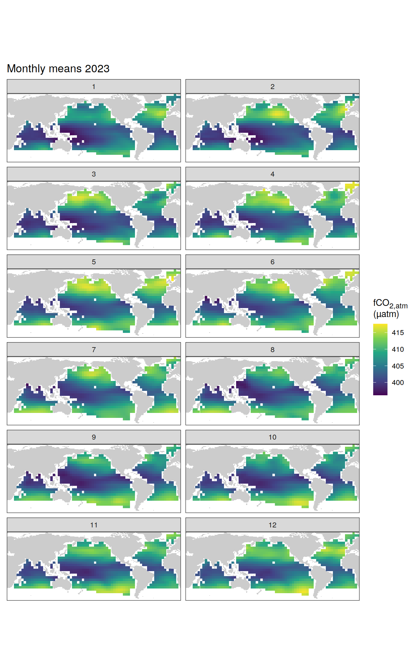
[[2]]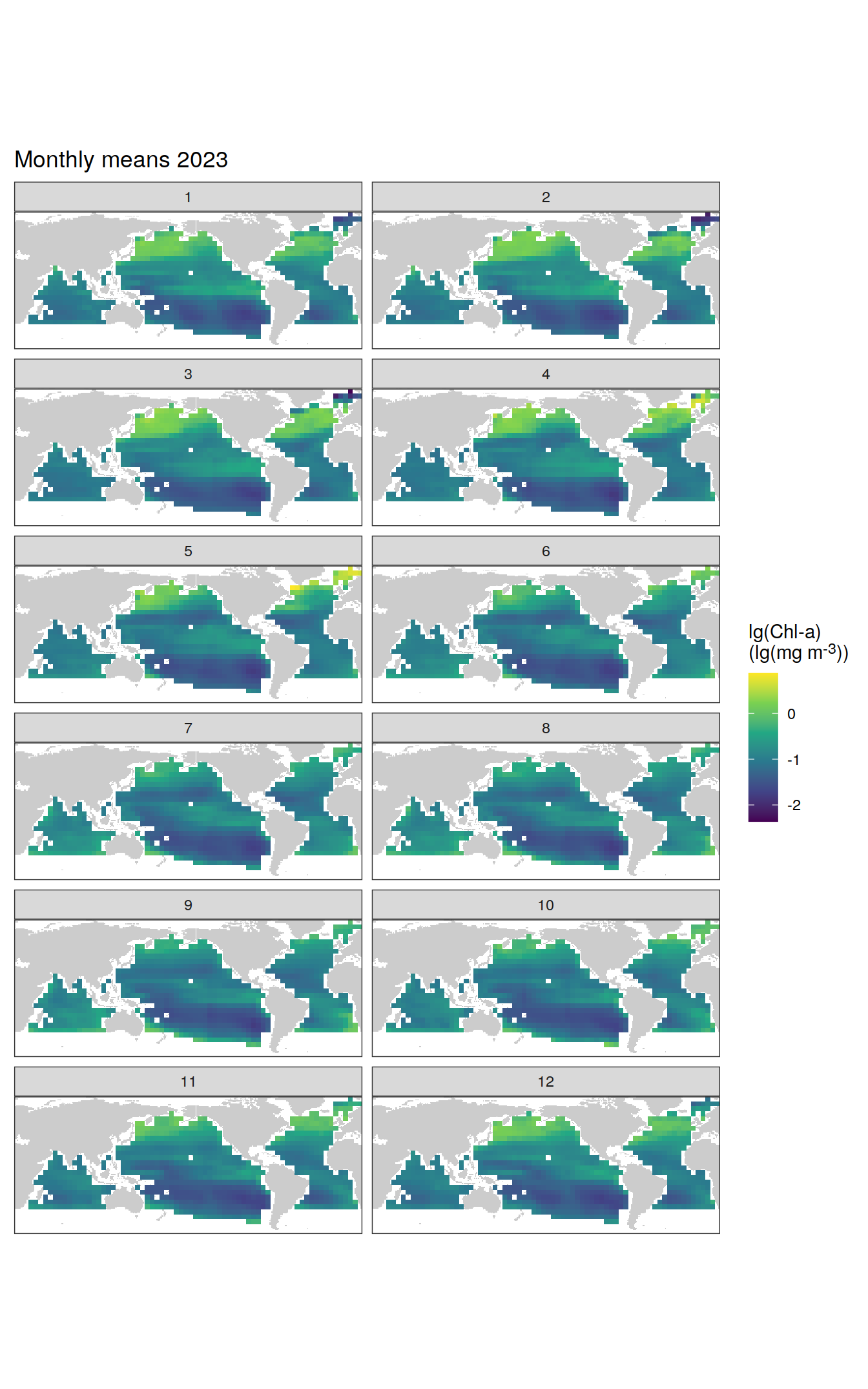
[[3]]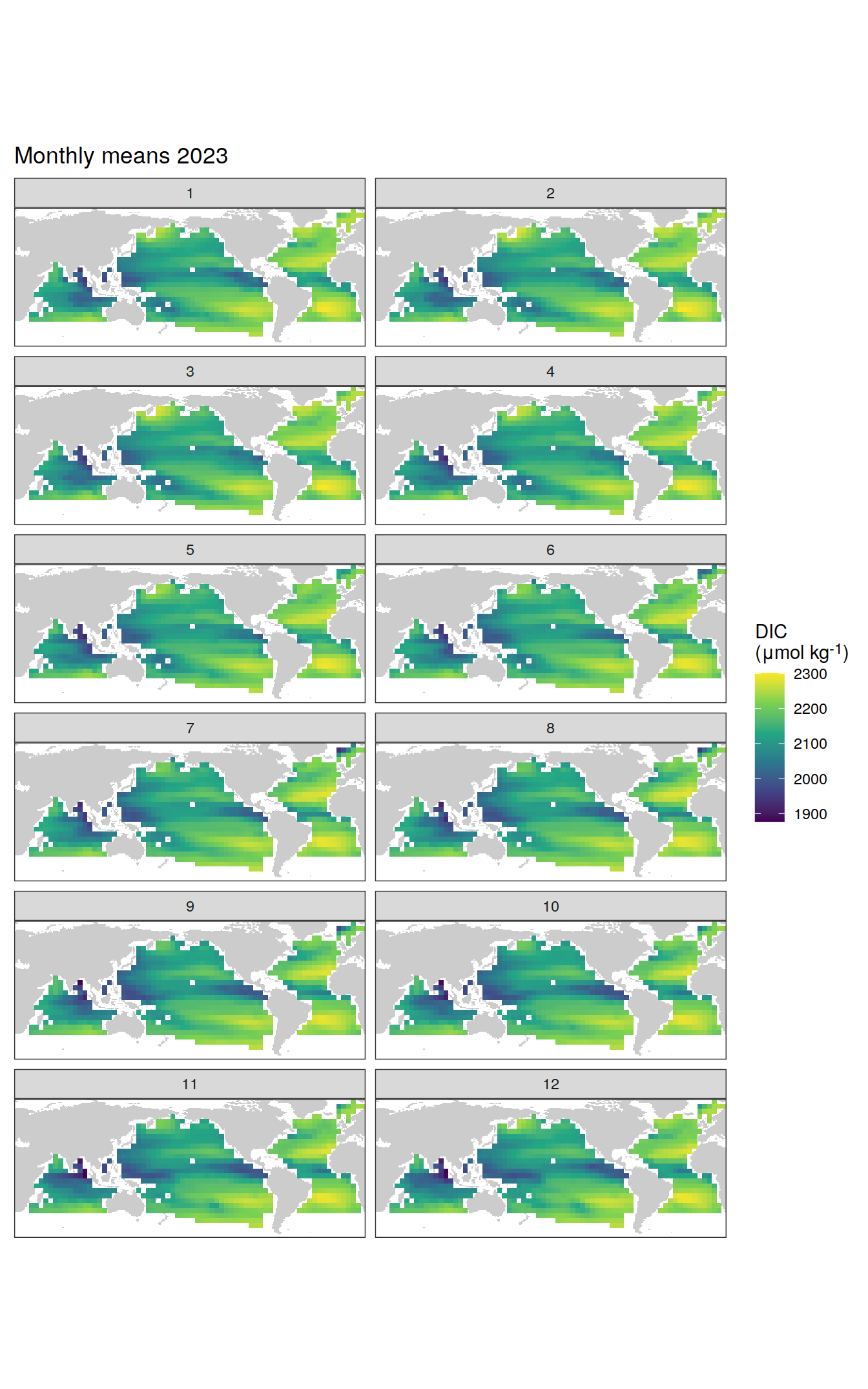
[[4]]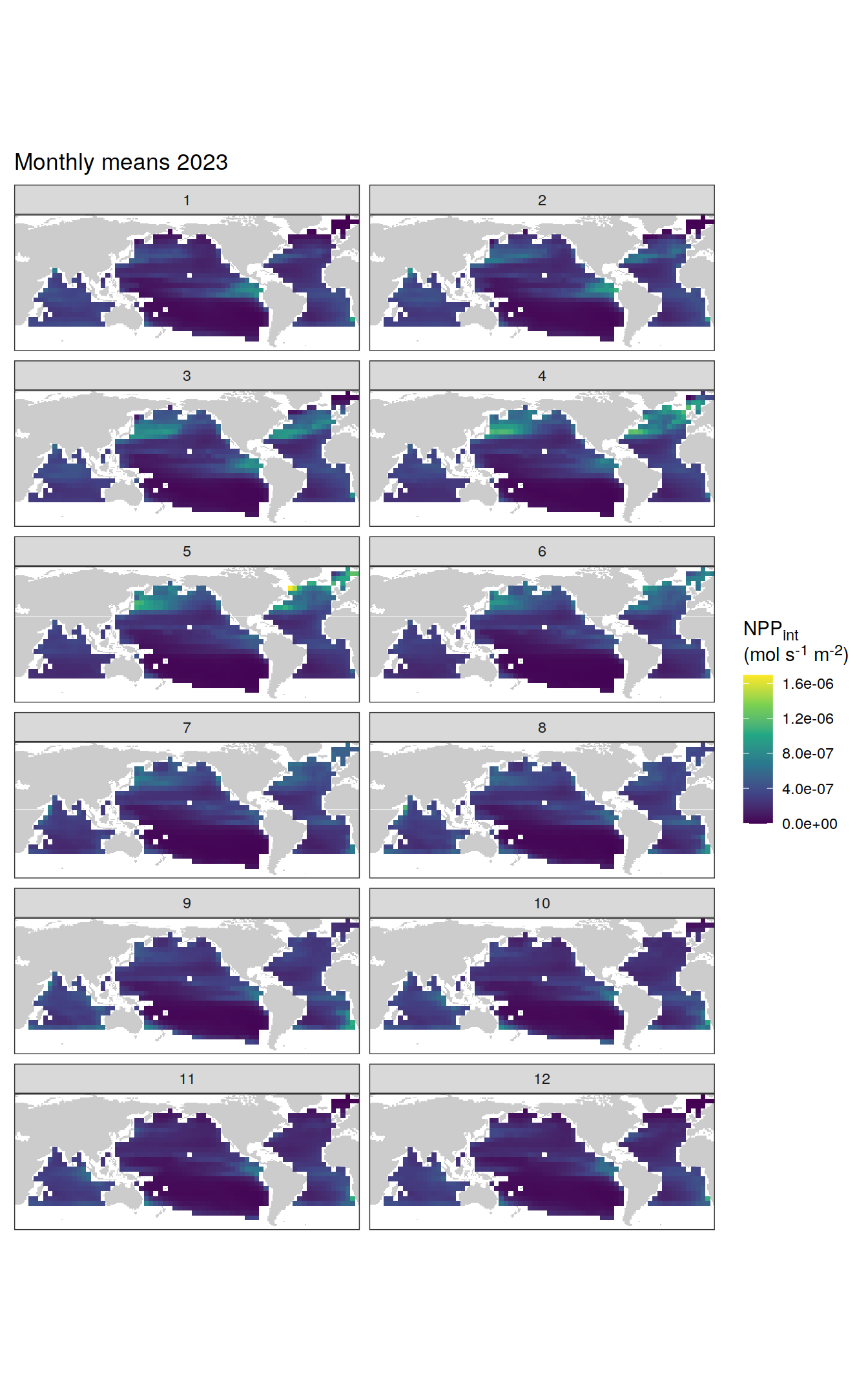
[[5]]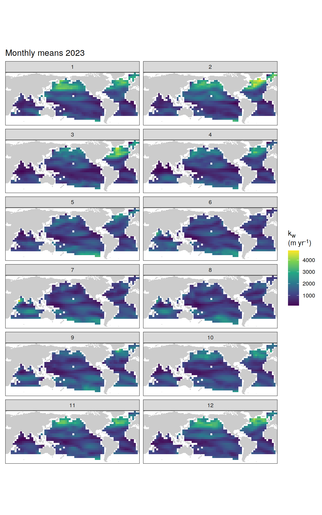
[[6]]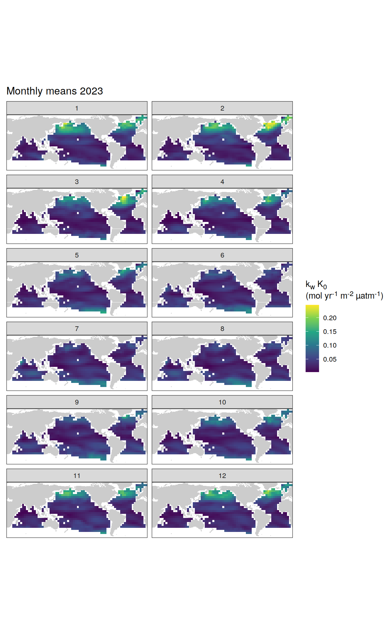
[[7]]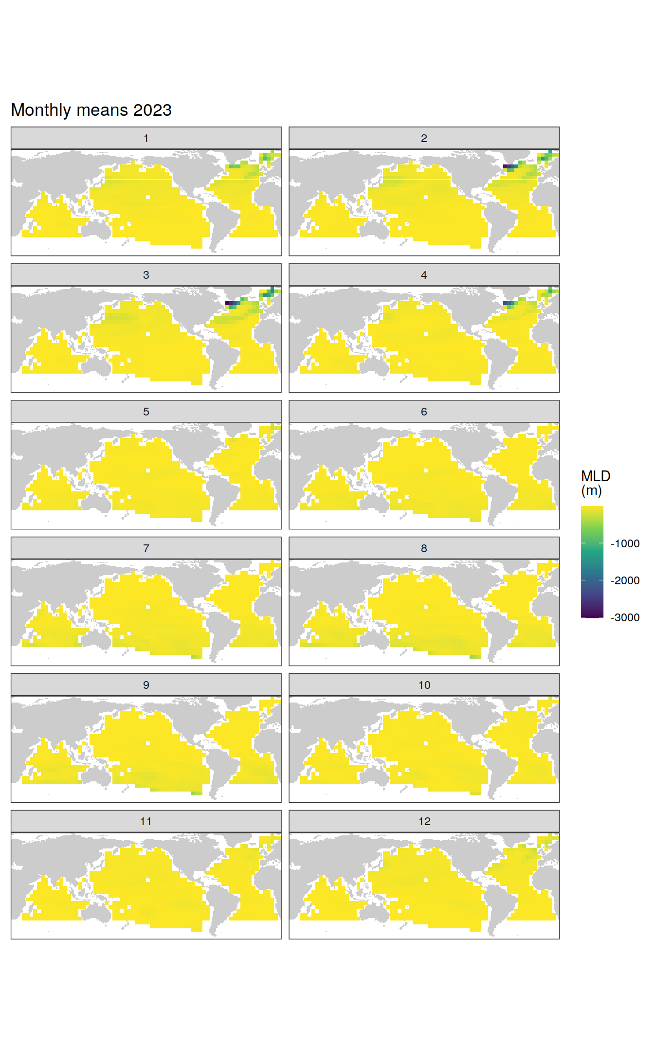
[[8]]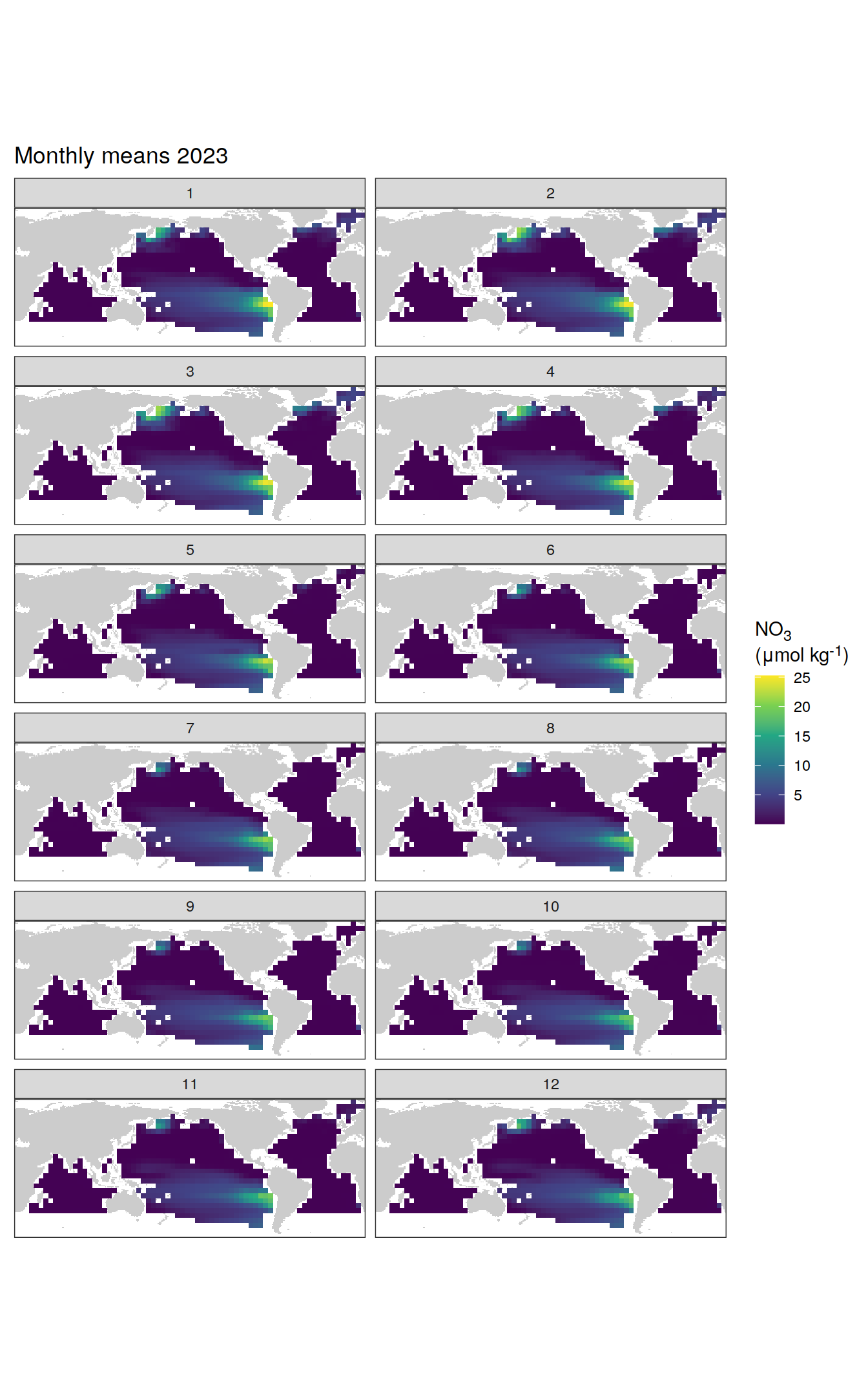
[[9]]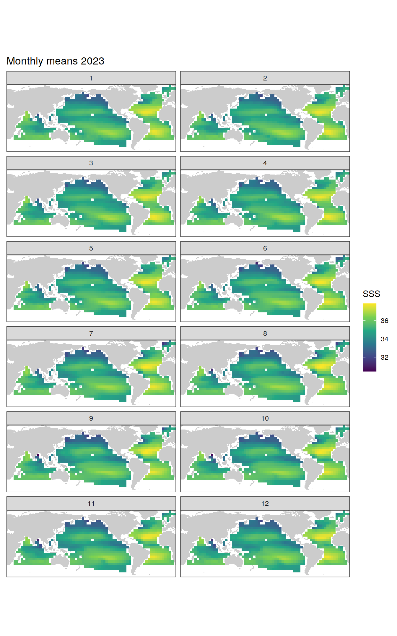
[[10]]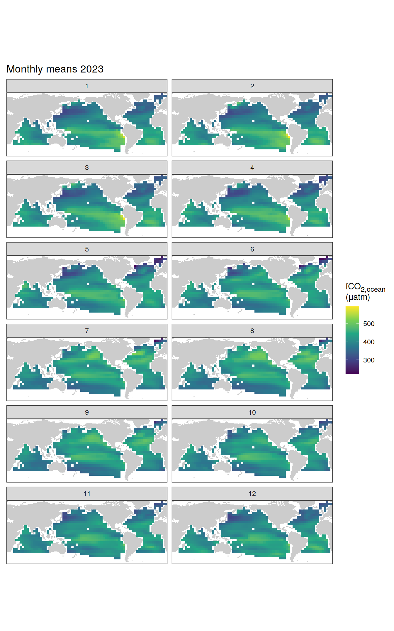
[[11]]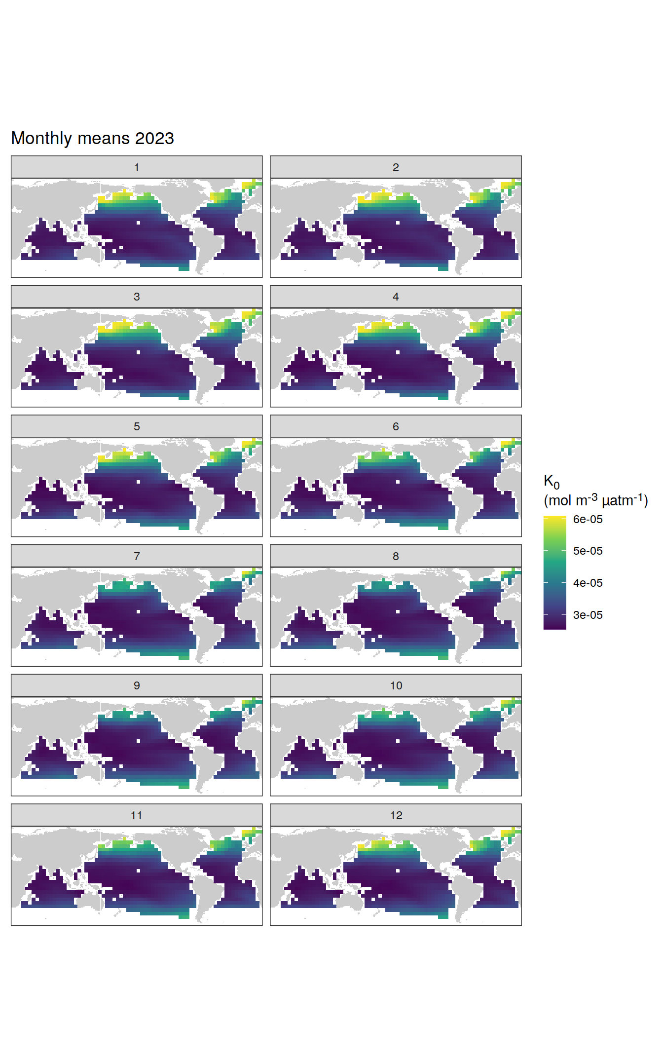
[[12]]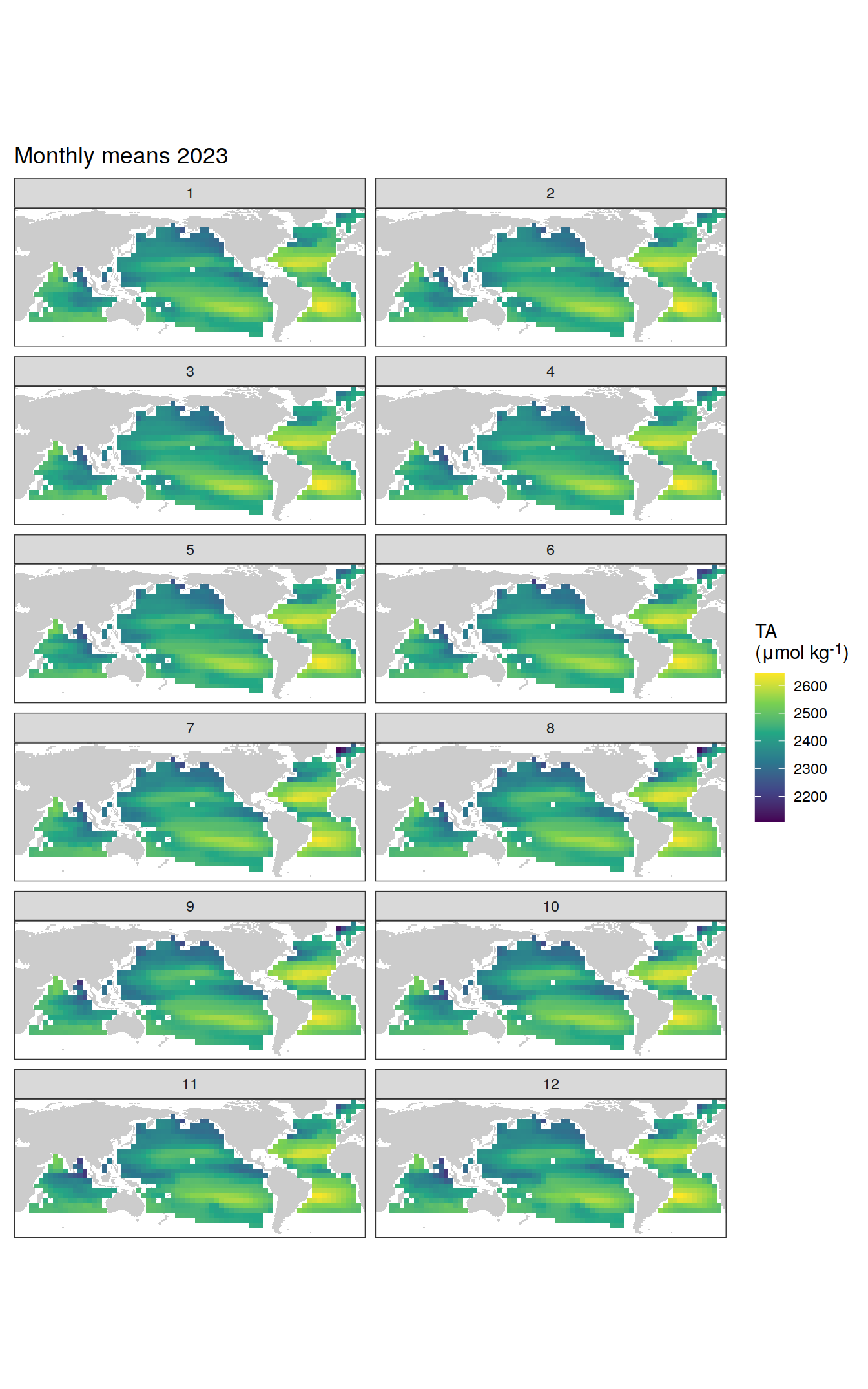
[[13]]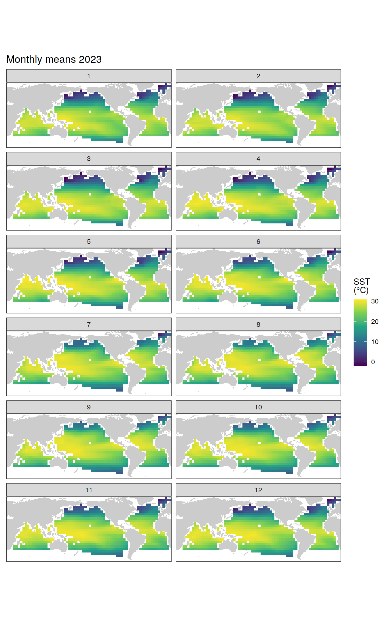
| Version | Author | Date |
|---|---|---|
| 054921b | jens-daniel-mueller | 2024-05-23 |
pco2_product_coarse_monthly_regression %>%
  filter(year == 2023,
         name %in% name_divergent) %>%
  group_split(name) %>%
  # head(1) %>%
  map(
    ~ map +
      geom_tile(data = .x,
                aes(lon, lat, fill = value)) +
      labs(title = paste("Monthly means", 2023)) +
      scale_fill_divergent(name = labels_breaks(.x %>% distinct(name))) +
      theme(legend.title = element_markdown()) +
      facet_wrap( ~ month, ncol = 2)
  )
[[1]]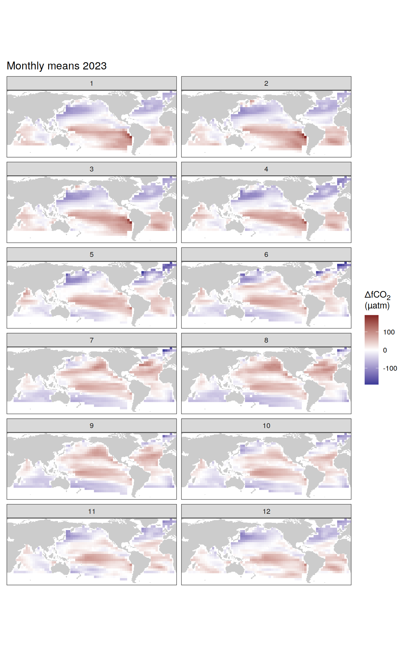
| Version | Author | Date |
|---|---|---|
| 054921b | jens-daniel-mueller | 2024-05-23 |
[[2]]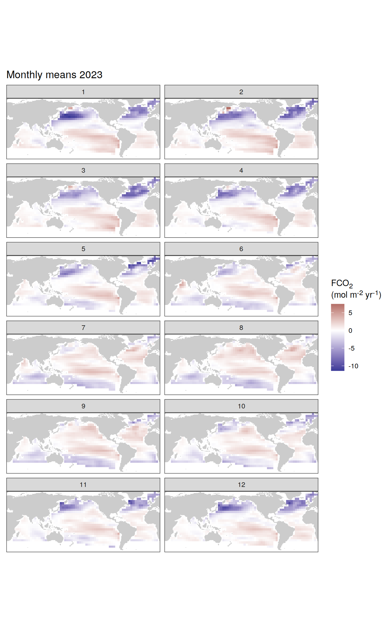
Trends
pco2_product_coarse_monthly_regression %>%
  group_by(name) %>%
  filter(year %in% c(min(year), max(year))) %>%
  ungroup() %>%
  select(-c(value, resid)) %>%
  arrange(year) %>%
  group_by(lon, lat, name, month) %>%
  mutate(change = fit - lag(fit),
         period = paste(lag(year), year, sep = "-")) %>%
  ungroup() %>%
  filter(!is.na(change)) %>%
  group_split(name) %>%
  # head(1) %>%
  map(
    ~ map +
      geom_tile(data = .x,
                aes(lon, lat, fill = change)) +
      labs(title =  paste("Change: ", .x$period)) +
      scale_fill_divergent(name = labels_breaks(.x %>% distinct(name))) +
      theme(legend.title = element_markdown()) +
      facet_wrap(~ month, ncol = 2)
  )
[[1]]
[[2]]
[[3]]
[[4]]
[[5]]
[[6]]
[[7]]
[[8]]
[[9]]
[[10]]
[[11]]
[[12]]
[[13]]
| Version | Author | Date |
|---|---|---|
| 054921b | jens-daniel-mueller | 2024-05-23 |
[[14]]
| Version | Author | Date |
|---|---|---|
| 054921b | jens-daniel-mueller | 2024-05-23 |
[[15]]
2023 anomaly
pco2_product_coarse_monthly_regression %>%
  filter(year == 2023) %>%
  group_split(name) %>%
  # head(1) %>%
  map(
    ~ map +
      geom_tile(data = .x,
                aes(lon, lat, fill = resid)) +
      labs(title = paste(2023, "anomaly")) +
      scale_fill_divergent(name = labels_breaks(.x %>% distinct(name))) +
      theme(legend.title = element_markdown()) +
      facet_wrap( ~ month, ncol = 2)
  )
[[1]]
[[2]]
[[3]]
[[4]]
[[5]]
[[6]]
[[7]]
[[8]]
[[9]]
[[10]]
[[11]]
[[12]]
[[13]]
| Version | Author | Date |
|---|---|---|
| 054921b | jens-daniel-mueller | 2024-05-23 |
[[14]]
| Version | Author | Date |
|---|---|---|
| 054921b | jens-daniel-mueller | 2024-05-23 |
[[15]]
pco2_product_coarse_monthly_regression %>%
  # filter(year == 2023) %>%
  write_csv(paste0("../data/","FESOM-REcoM","_","2023","_anomaly_map_monthly.csv"))
Hovmoeller plots
The following Hovmoeller plots show the anomalies from the prediction of the linear/quadratic fits.
Hovmoeller plots are first presented as annual means, and than as monthly means. Note that the predictions for the monthly Hovmoeller plots are done individually for each month, such the mean seasonal anomaly from the annual mean is removed.
2023 annual anomalies
pco2_product_hovmoeller_monthly_annual_regression <-
  pco2_product_hovmoeller_monthly_annual %>%
  anomaly_determination(lat) %>%
  filter(!is.na(resid))


pco2_product_hovmoeller_monthly_annual_regression %>%
  # filter(name == "mld") %>%
  group_split(name) %>%
  # head(1) %>%
  map(
    ~ ggplot(data = .x,
             aes(year, lat, fill = resid)) +
      geom_raster() +
      scale_fill_divergent(name = labels_breaks(.x %>% distinct(name))) +
      theme(legend.title = element_markdown()) +
      coord_cartesian(expand = 0) +
      labs(title = "Annual mean anomalies",
           y = "Latitude") +
      theme(axis.title.x = element_blank())
  )
[[1]]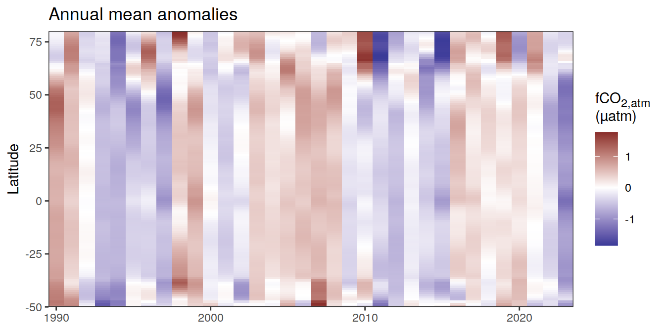
[[2]]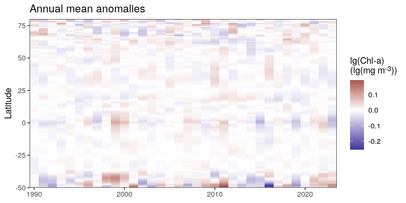
[[3]]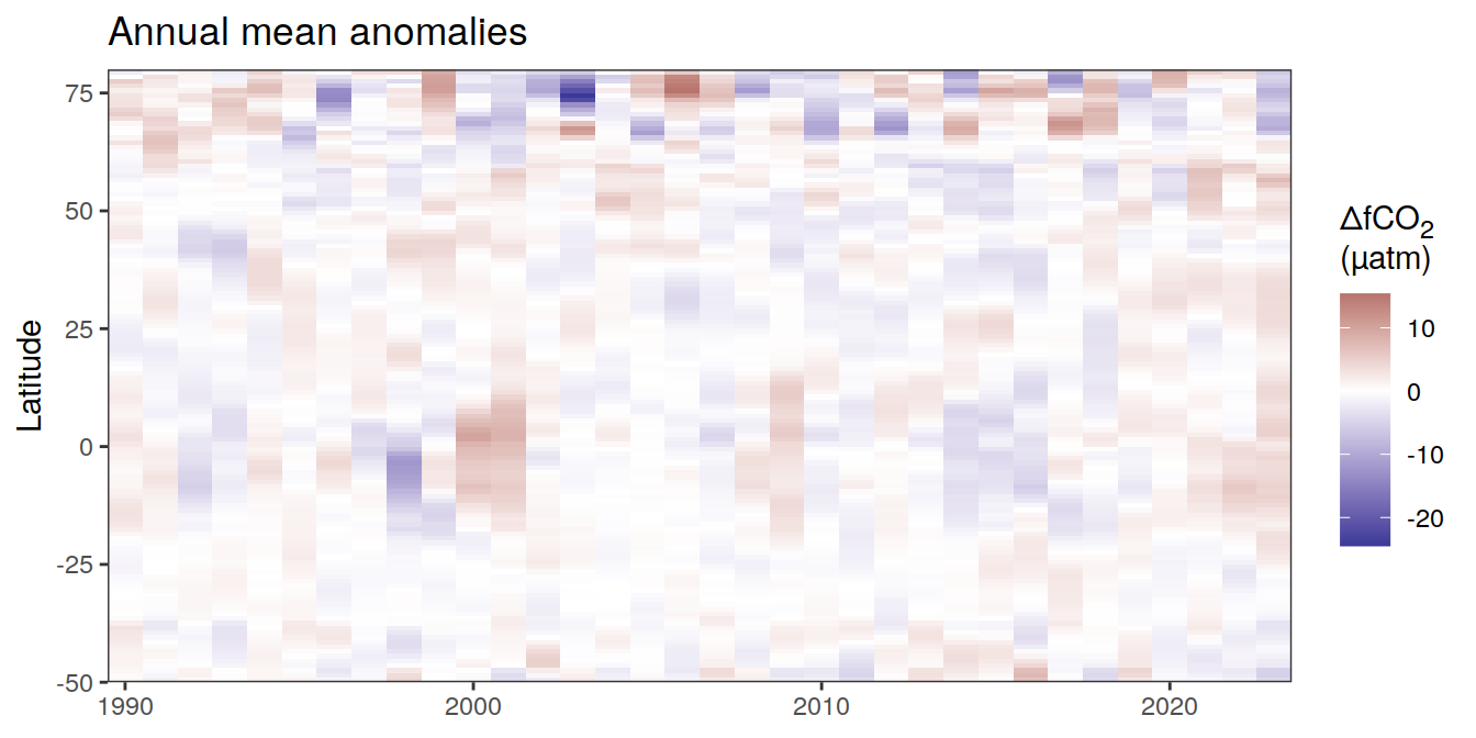
[[4]]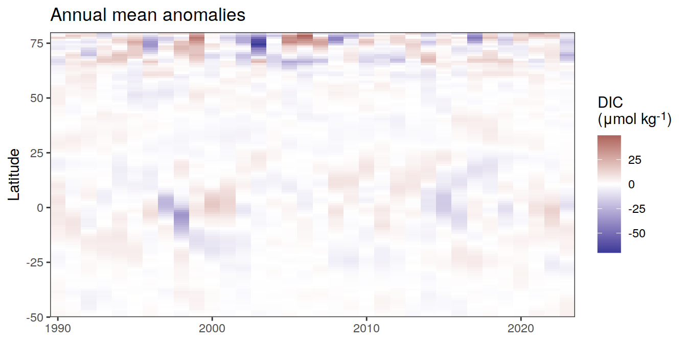
[[5]]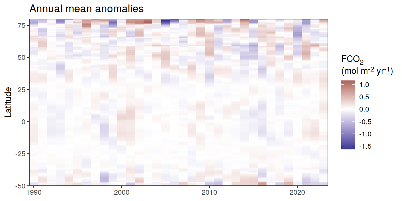
[[6]]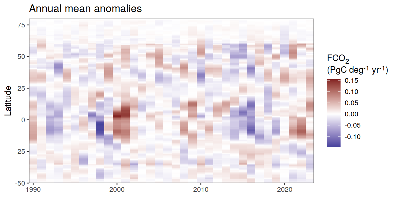
[[7]]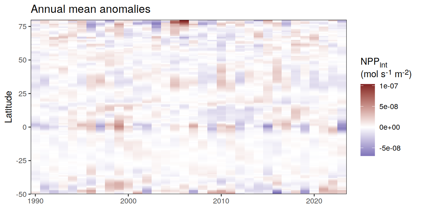
[[8]]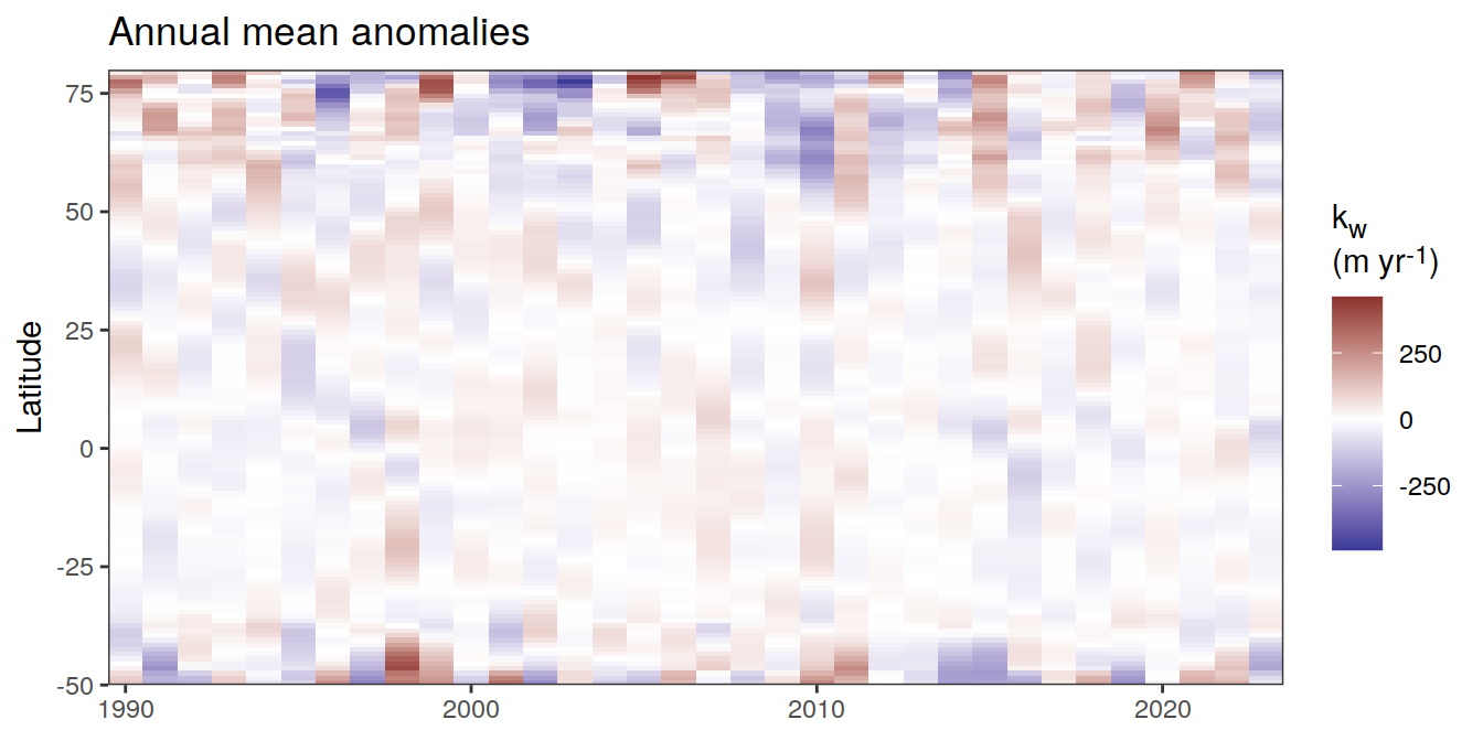
[[9]]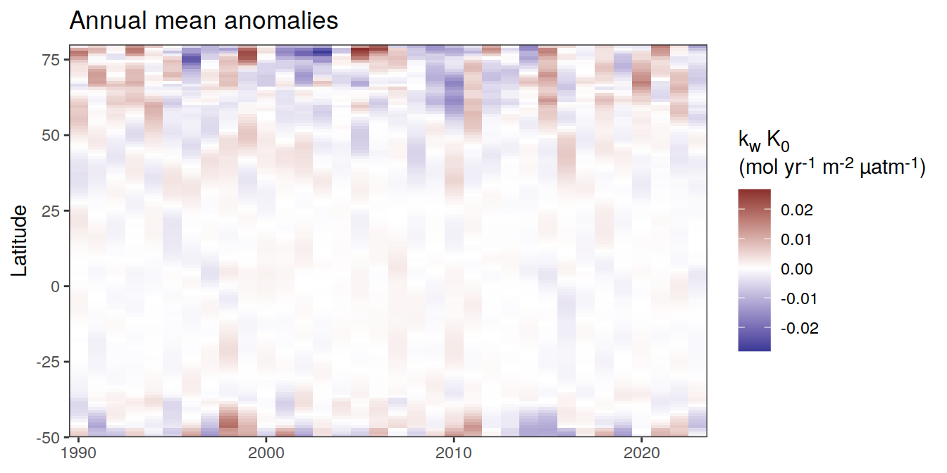
[[10]]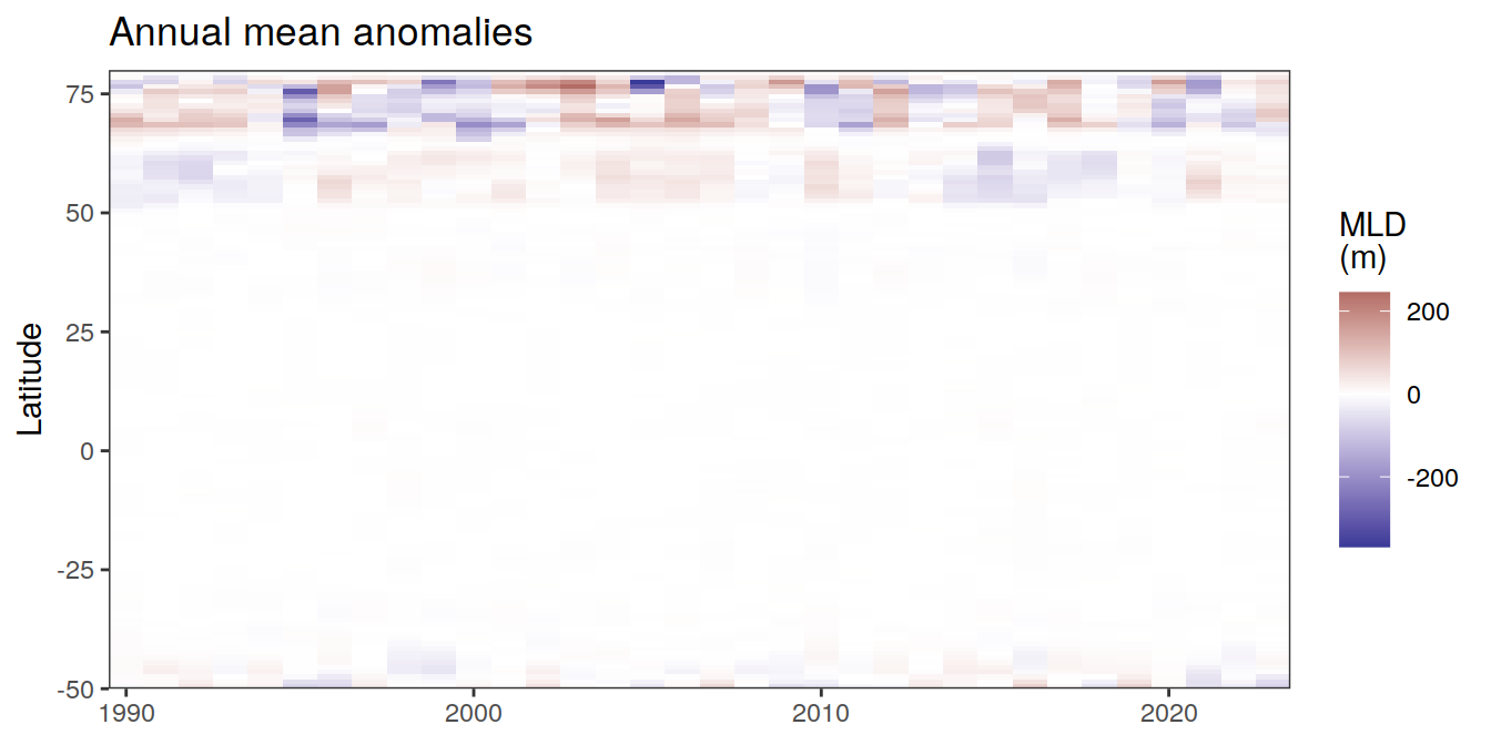
[[11]]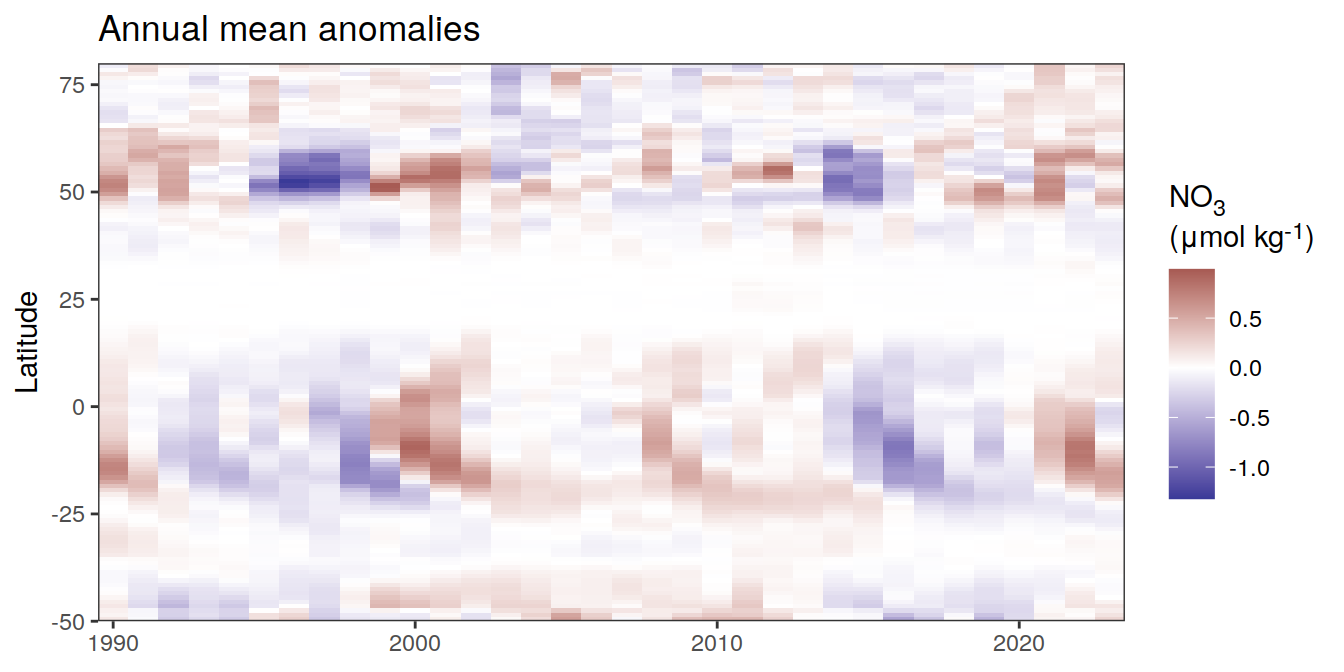
[[12]]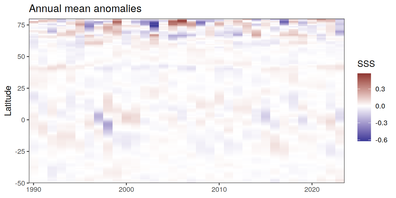
[[13]]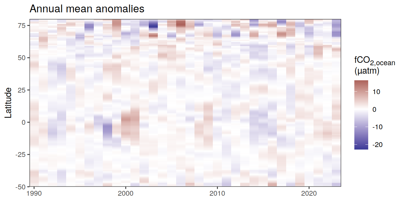
[[14]]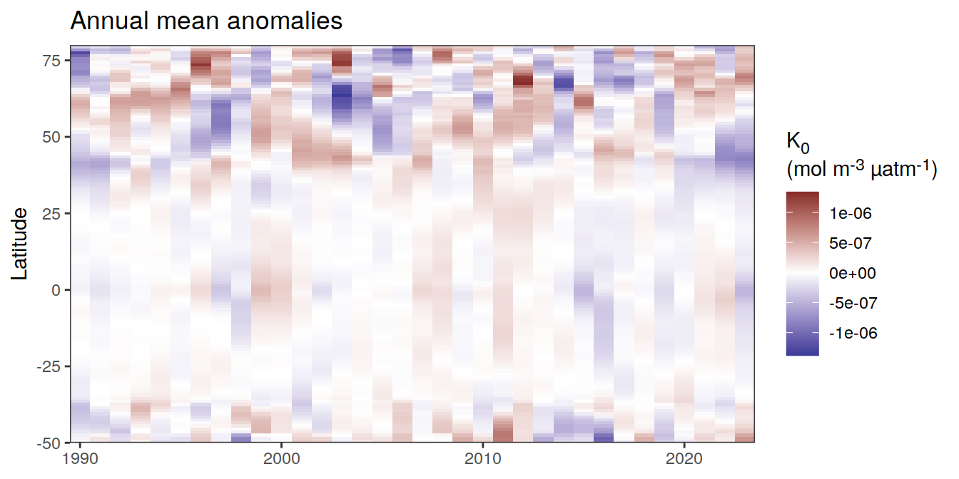
| Version | Author | Date |
|---|---|---|
| 054921b | jens-daniel-mueller | 2024-05-23 |
[[15]]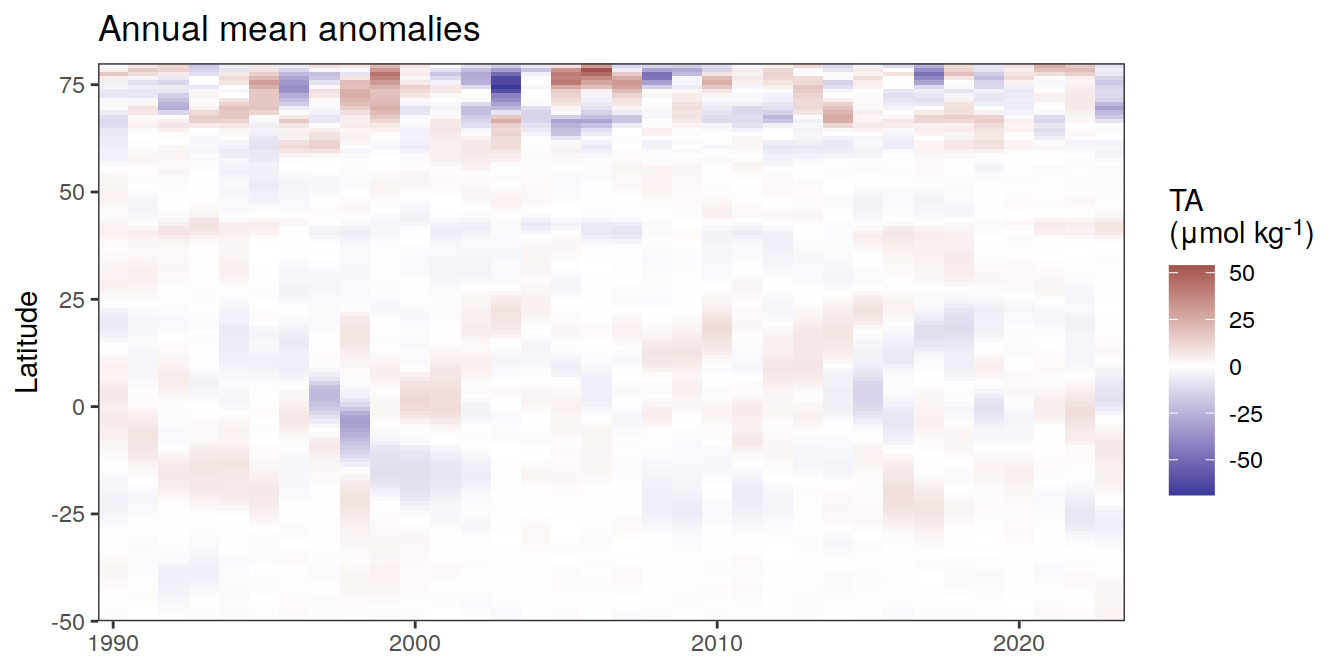
| Version | Author | Date |
|---|---|---|
| 054921b | jens-daniel-mueller | 2024-05-23 |
[[16]]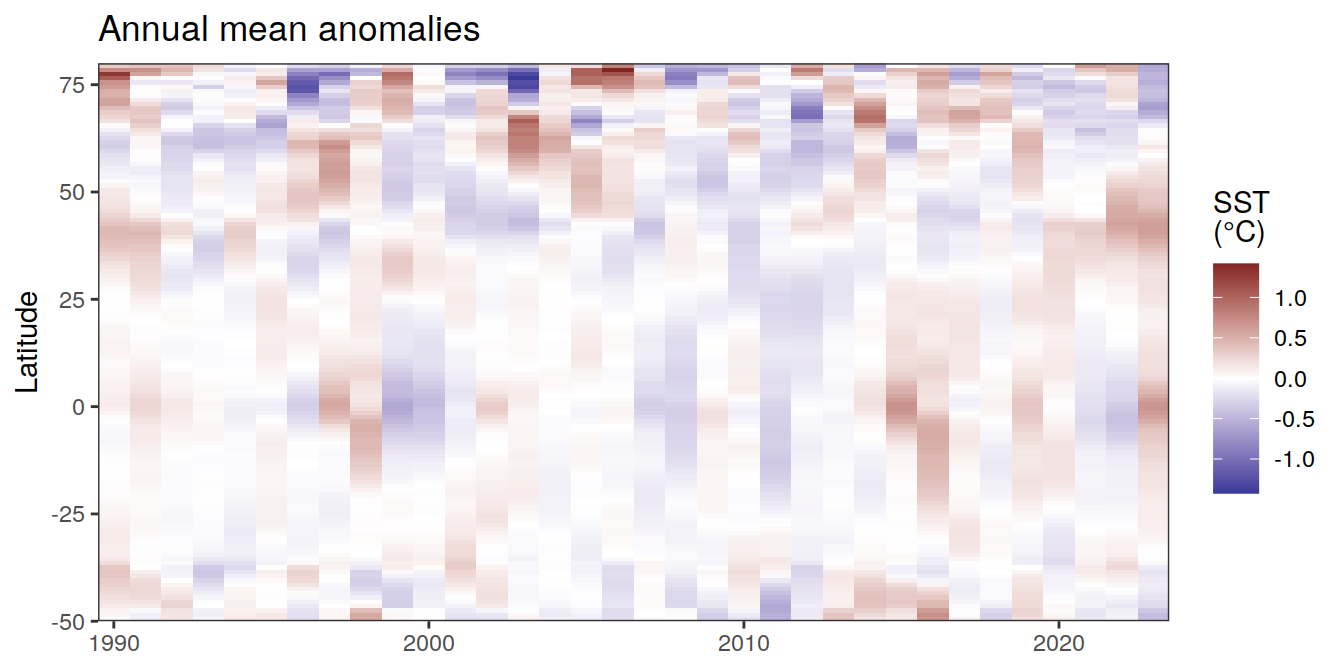
2023 monthly anomalies
pco2_product_hovmoeller_monthly_regression <-
  pco2_product_hovmoeller_monthly %>%
  select(-c(decimal)) %>%
  anomaly_determination(lat, month) %>%
  filter(!is.na(resid))


pco2_product_hovmoeller_monthly_regression <-
  pco2_product_hovmoeller_monthly_regression %>%
  mutate(decimal = year + (month - 1) / 12)

pco2_product_hovmoeller_monthly_regression %>%
  group_split(name) %>%
  # head(1) %>%
  map(
    ~ ggplot(data = .x,
             aes(decimal, lat, fill = resid)) +
      geom_raster() +
      scale_fill_divergent(name = labels_breaks(.x %>% distinct(name))) +
      theme(legend.title = element_markdown()) +
      coord_cartesian(expand = 0) +
      labs(title = "Monthly mean anomalies",
           y = "Latitude") +
      theme(axis.title.x = element_blank())
  )
[[1]]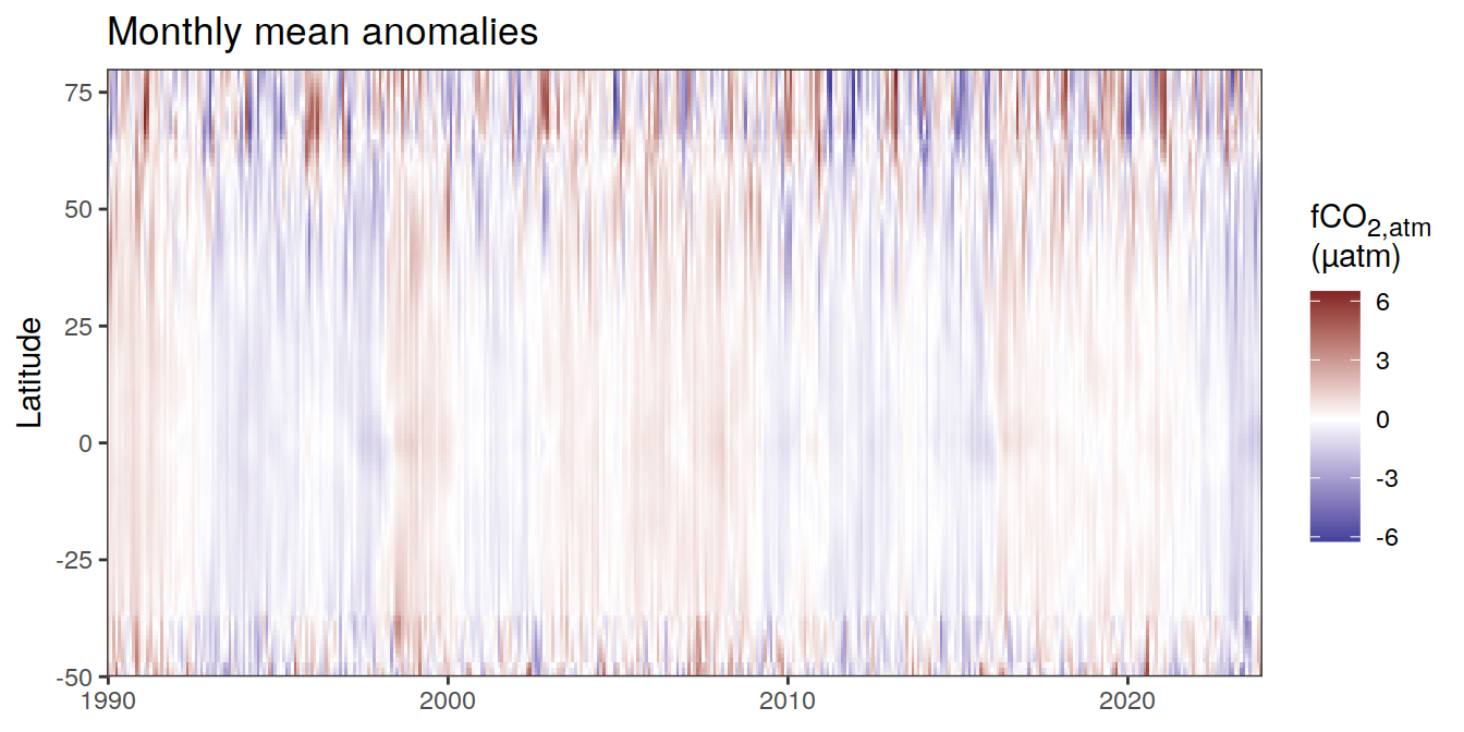
[[2]]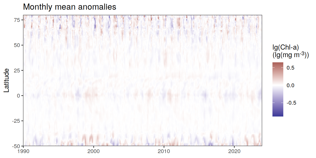
[[3]]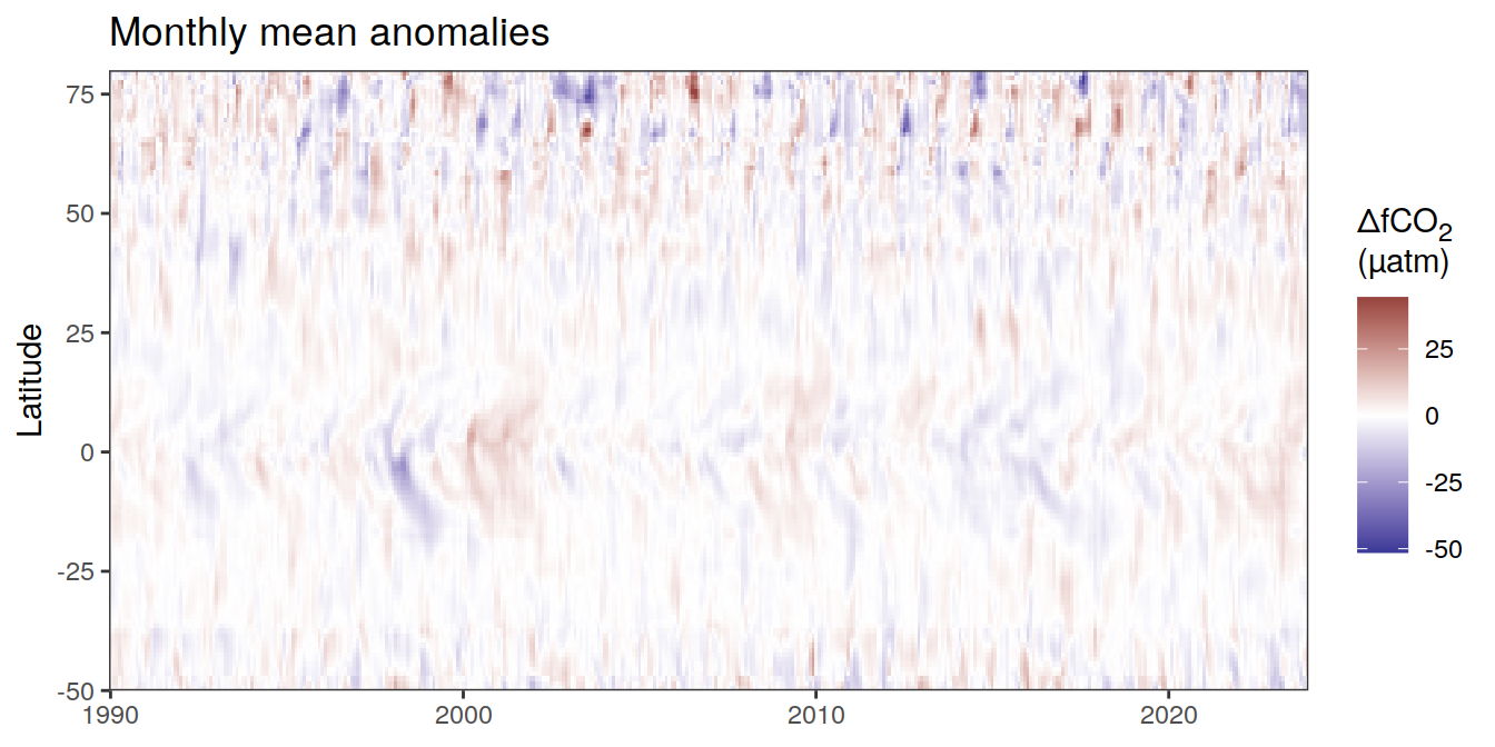
[[4]]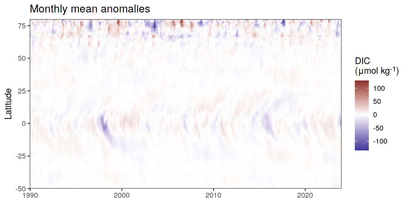
[[5]]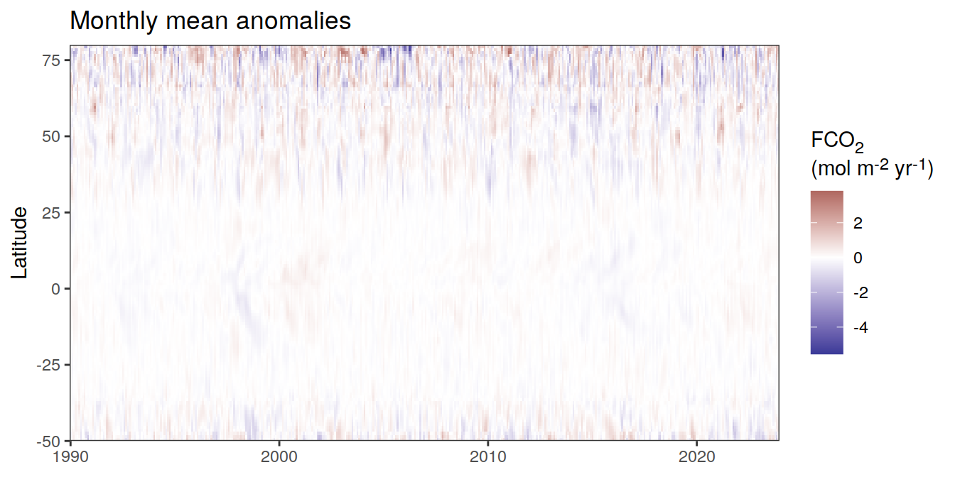
[[6]]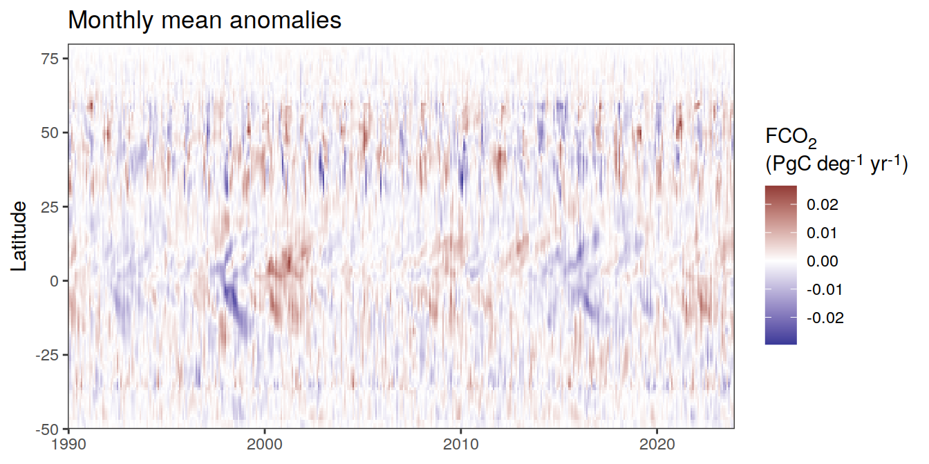
[[7]]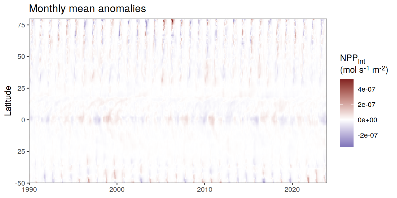
[[8]]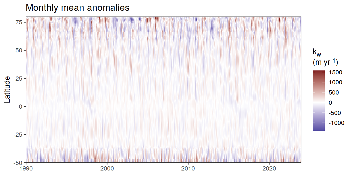
[[9]]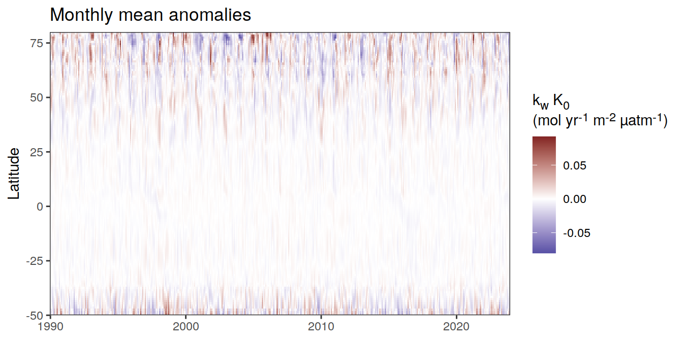
[[10]]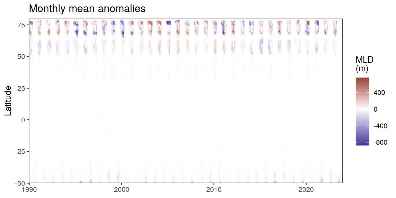
[[11]]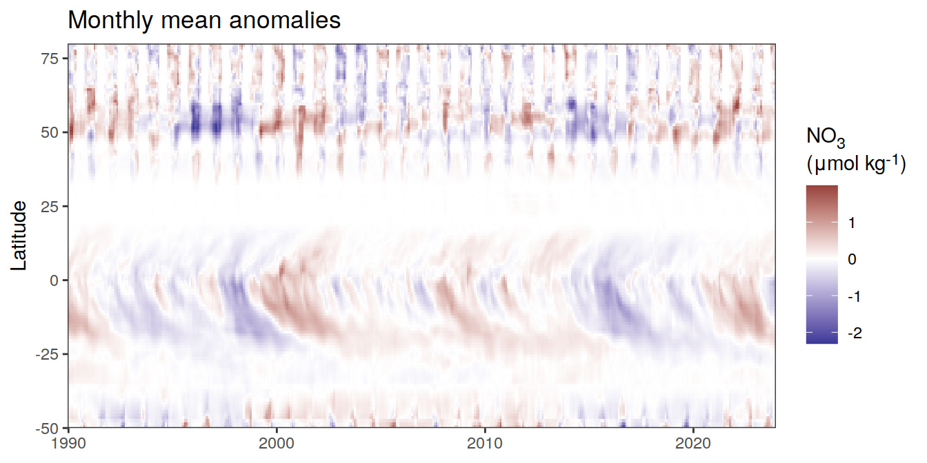
[[12]]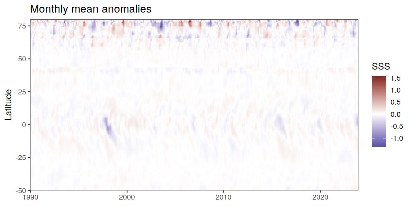
[[13]]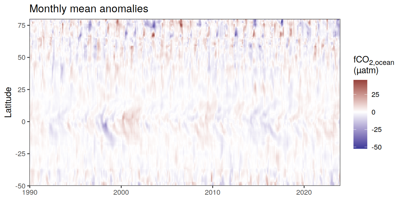
[[14]]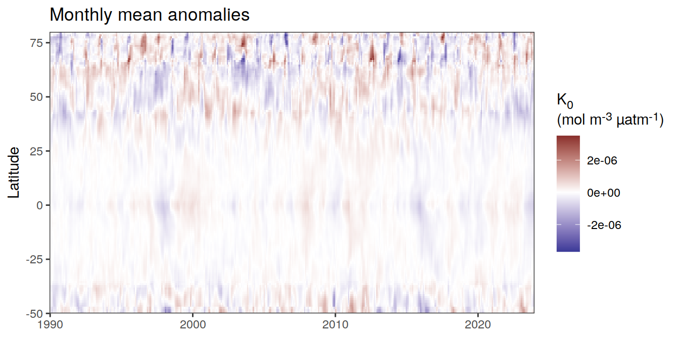
| Version | Author | Date |
|---|---|---|
| 054921b | jens-daniel-mueller | 2024-05-23 |
[[15]]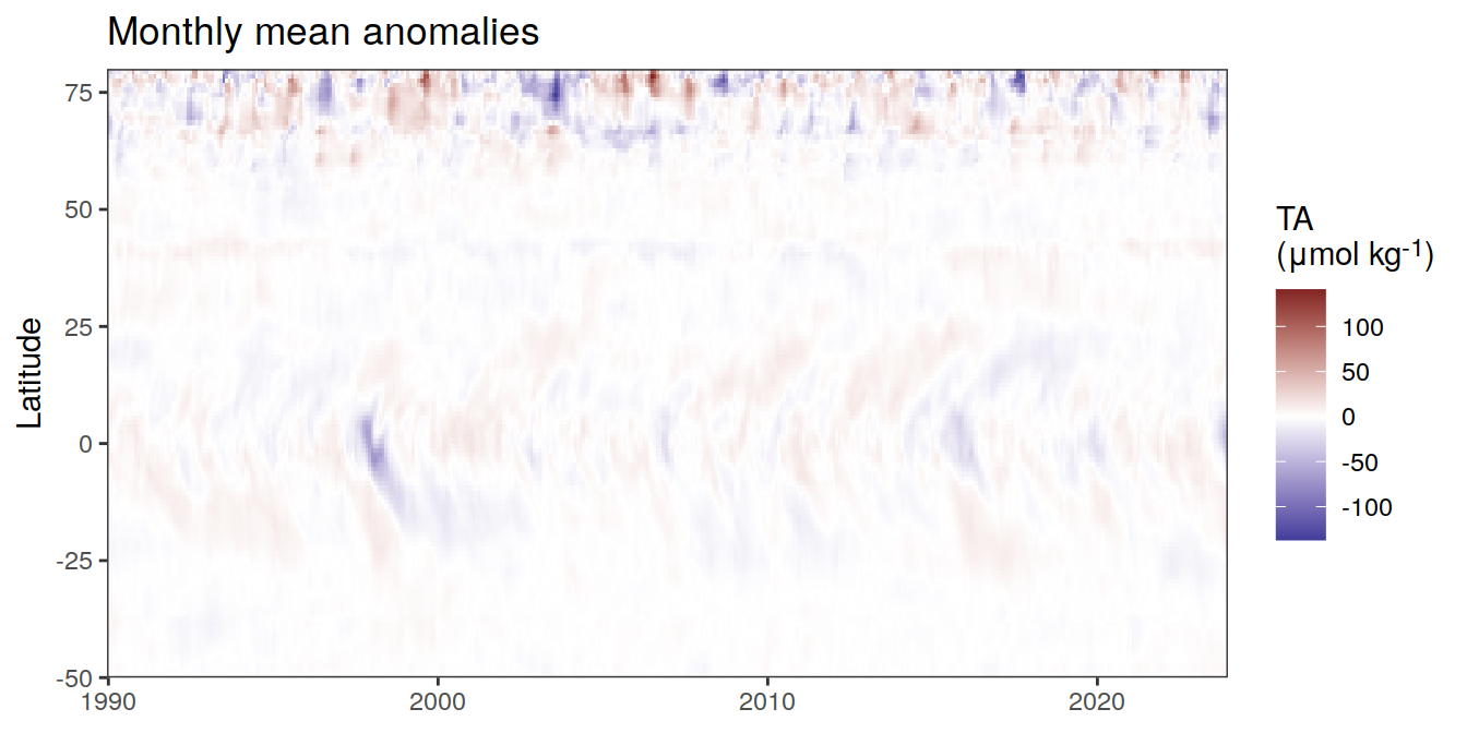
| Version | Author | Date |
|---|---|---|
| 054921b | jens-daniel-mueller | 2024-05-23 |
[[16]]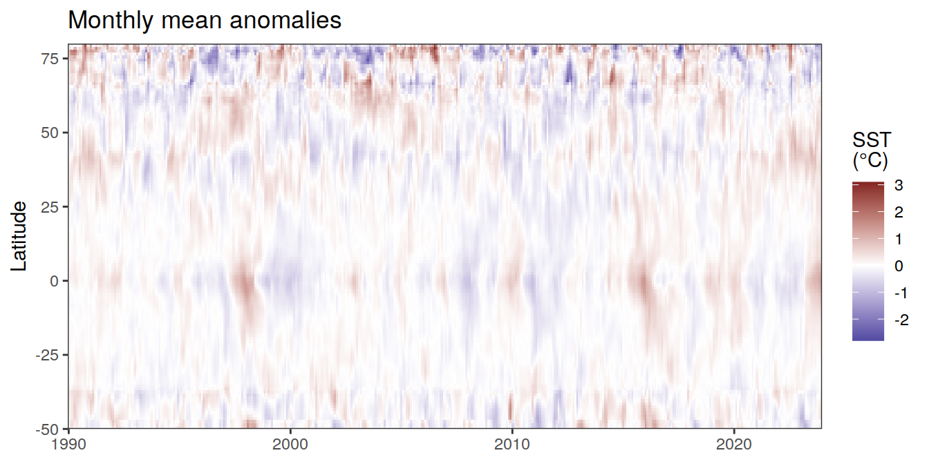
pco2_product_hovmoeller_monthly_regression %>%
  write_csv(paste0("../data/","FESOM-REcoM","_","2023","_anomaly_hovmoeller_monthly.csv"))
Three years prior 2023
pco2_product_hovmoeller_monthly_regression %>%
  filter(between(year, 2023-2, 2023)) %>%
  group_split(name) %>%
  # head(1) %>%
  map(
    ~ ggplot(data = .x,
             aes(decimal, lat, fill = resid)) +
      geom_raster() +
      scale_fill_divergent(name = labels_breaks(.x %>% distinct(name))) +
      theme(legend.title = element_markdown()) +
      coord_cartesian(expand = 0) +
      labs(title = "Monthly mean anomalies",
           y = "Latitude") +
      theme(axis.title.x = element_blank())
  )
[[1]]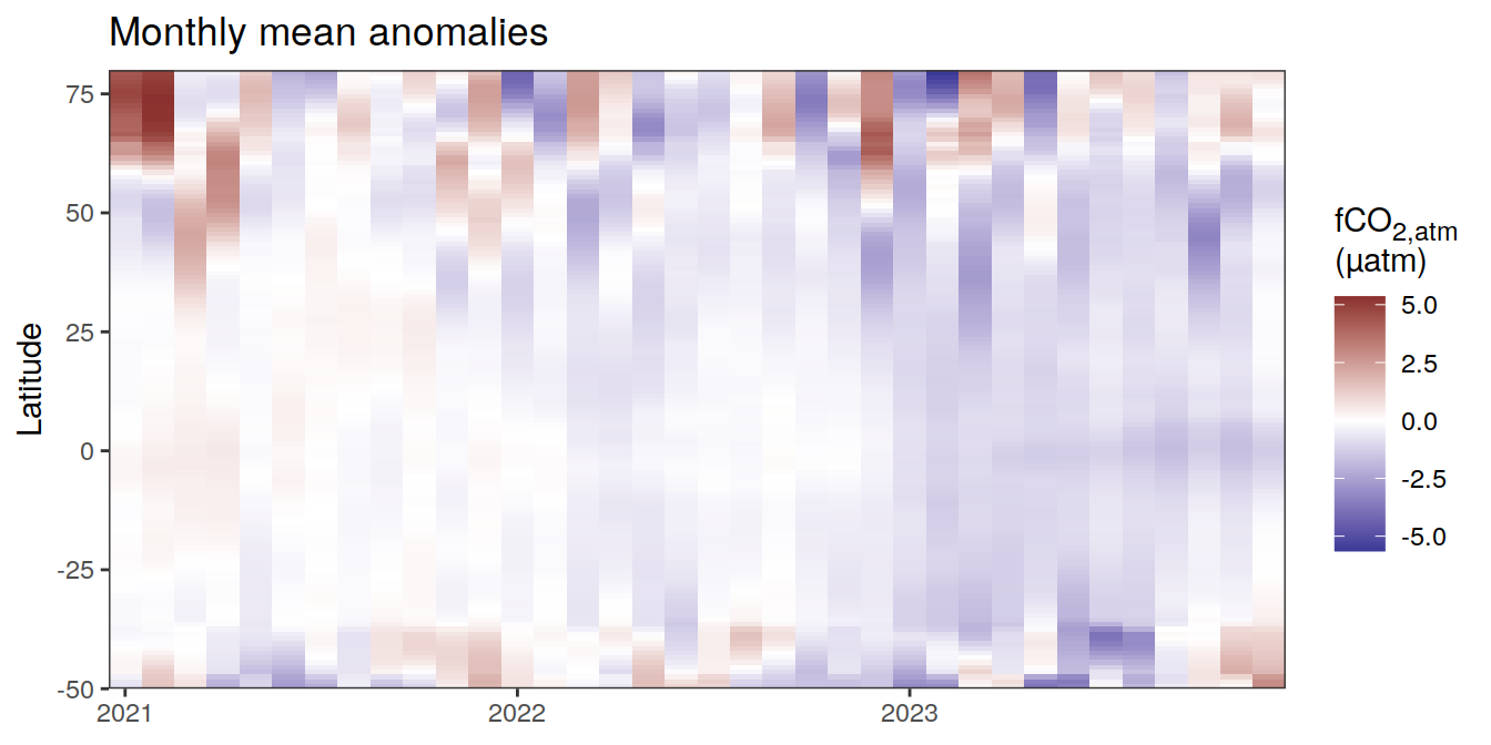
[[2]]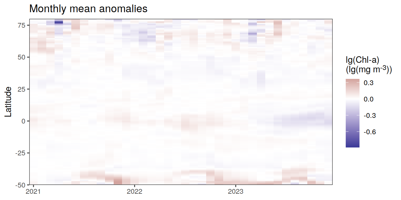
[[3]]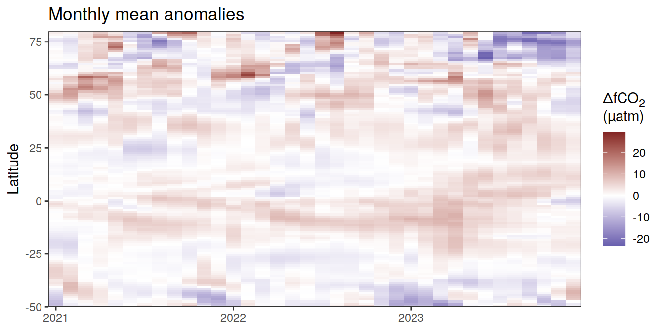
[[4]]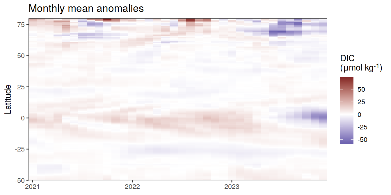
[[5]]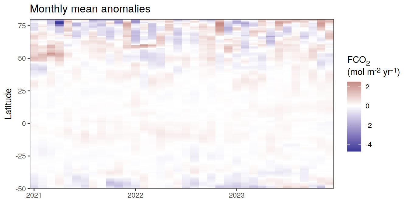
[[6]]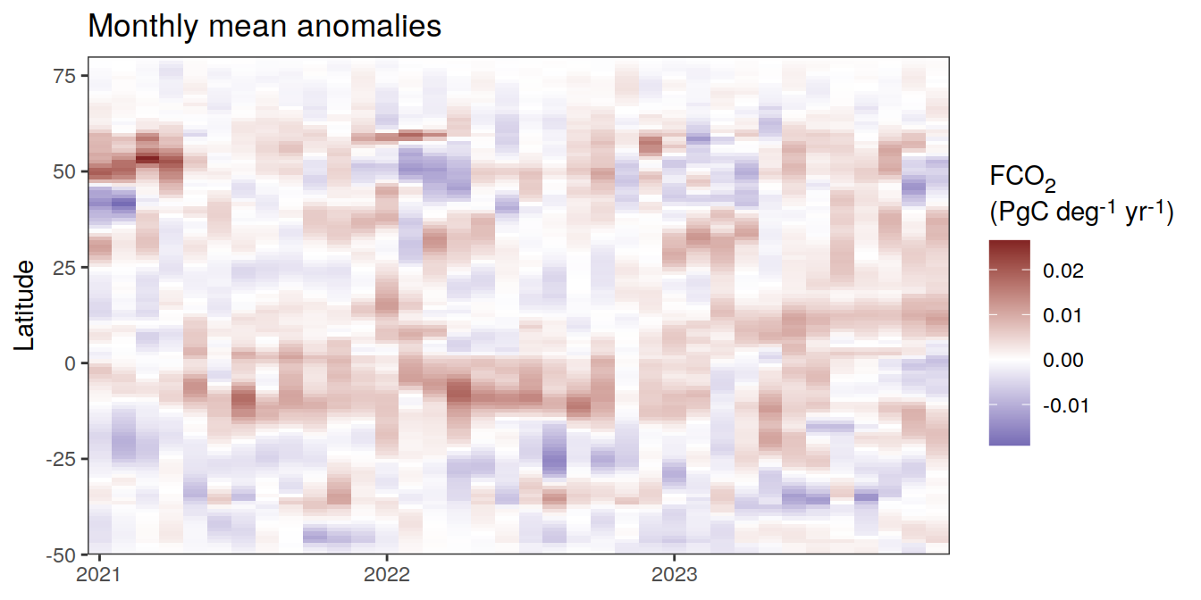
[[7]]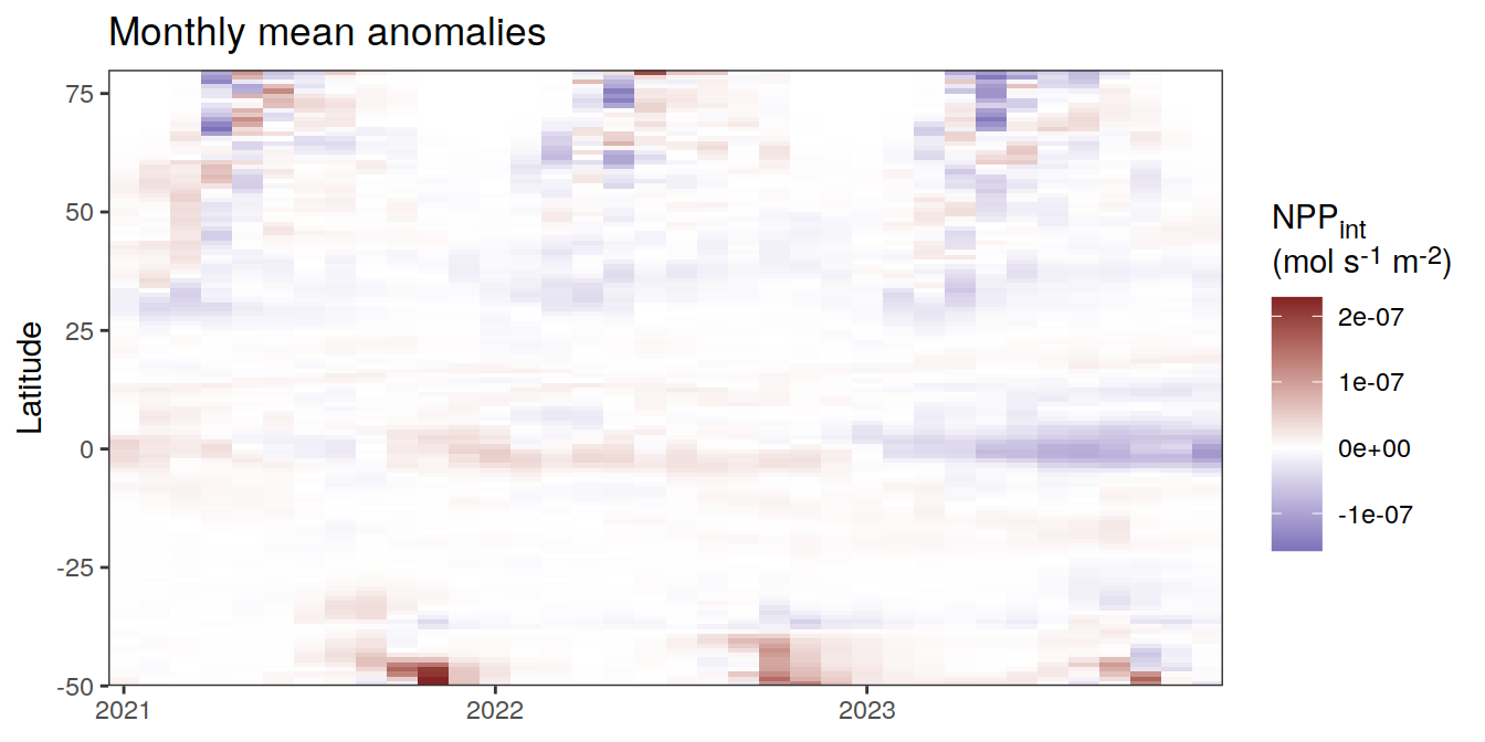
[[8]]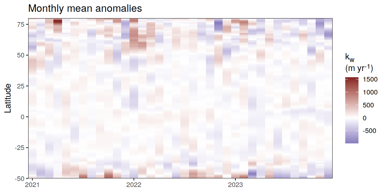
[[9]]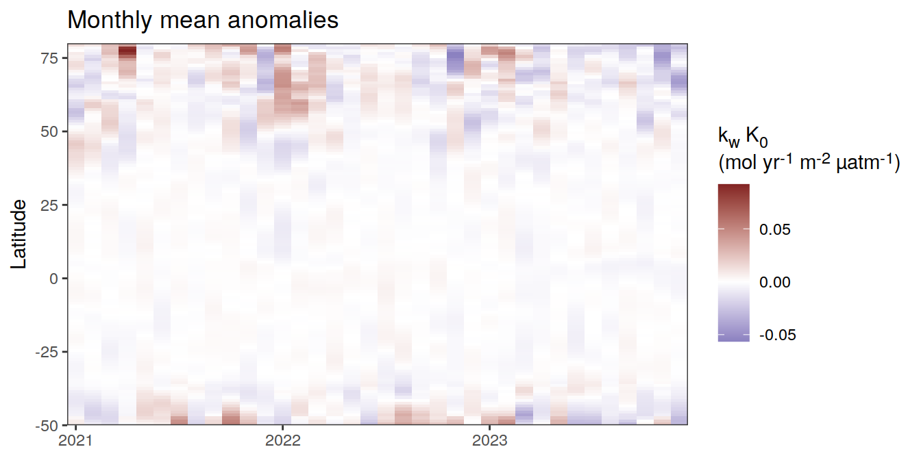
[[10]]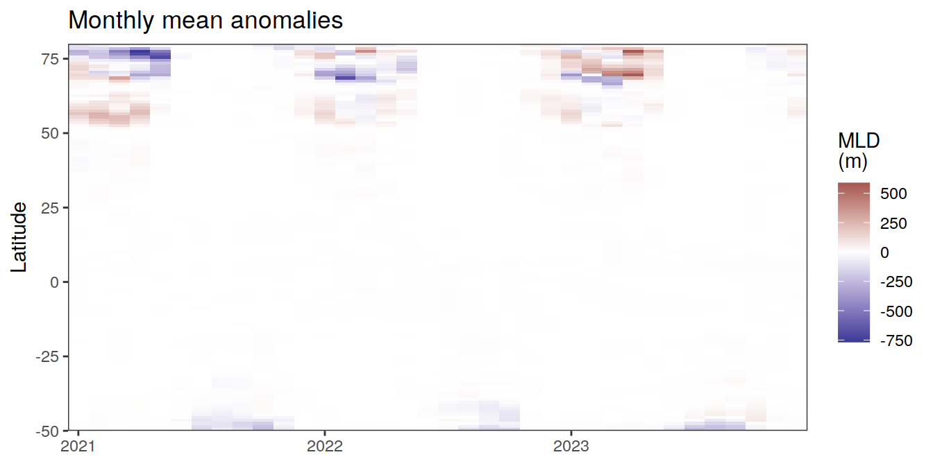
[[11]]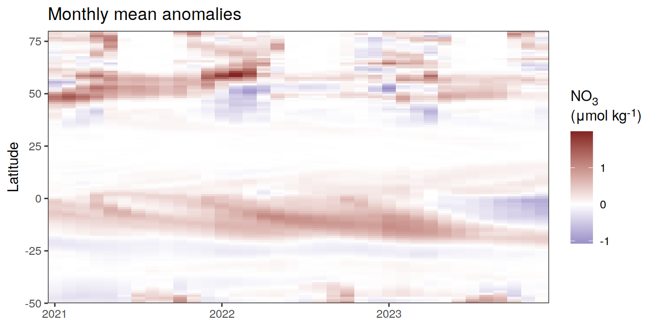
[[12]]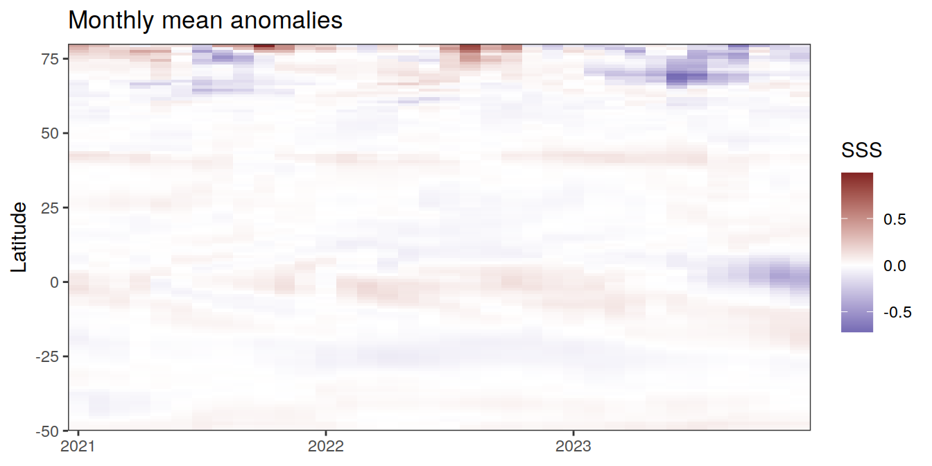
[[13]]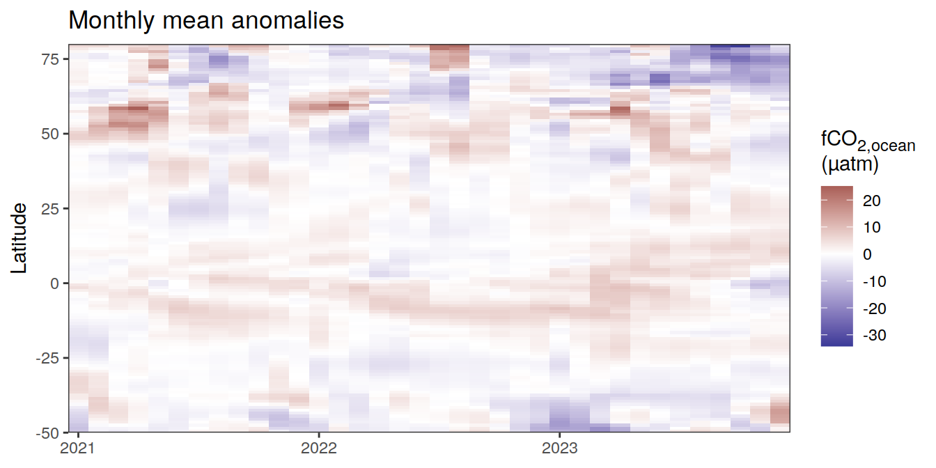
[[14]]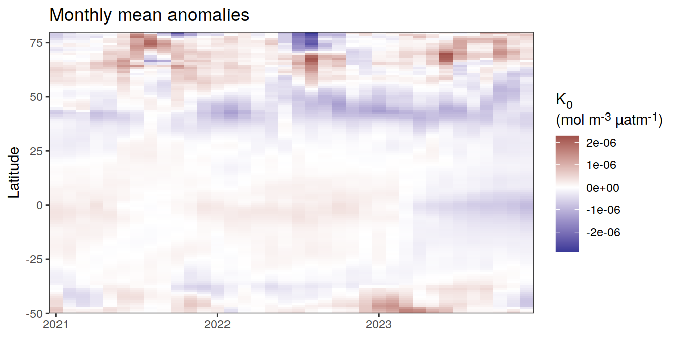
| Version | Author | Date |
|---|---|---|
| 054921b | jens-daniel-mueller | 2024-05-23 |
[[15]]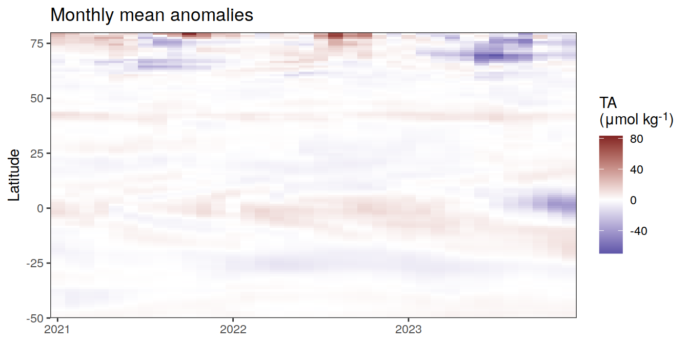
| Version | Author | Date |
|---|---|---|
| 054921b | jens-daniel-mueller | 2024-05-23 |
[[16]]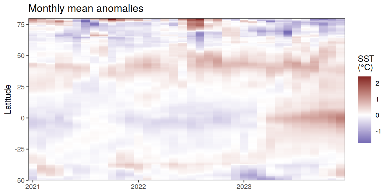
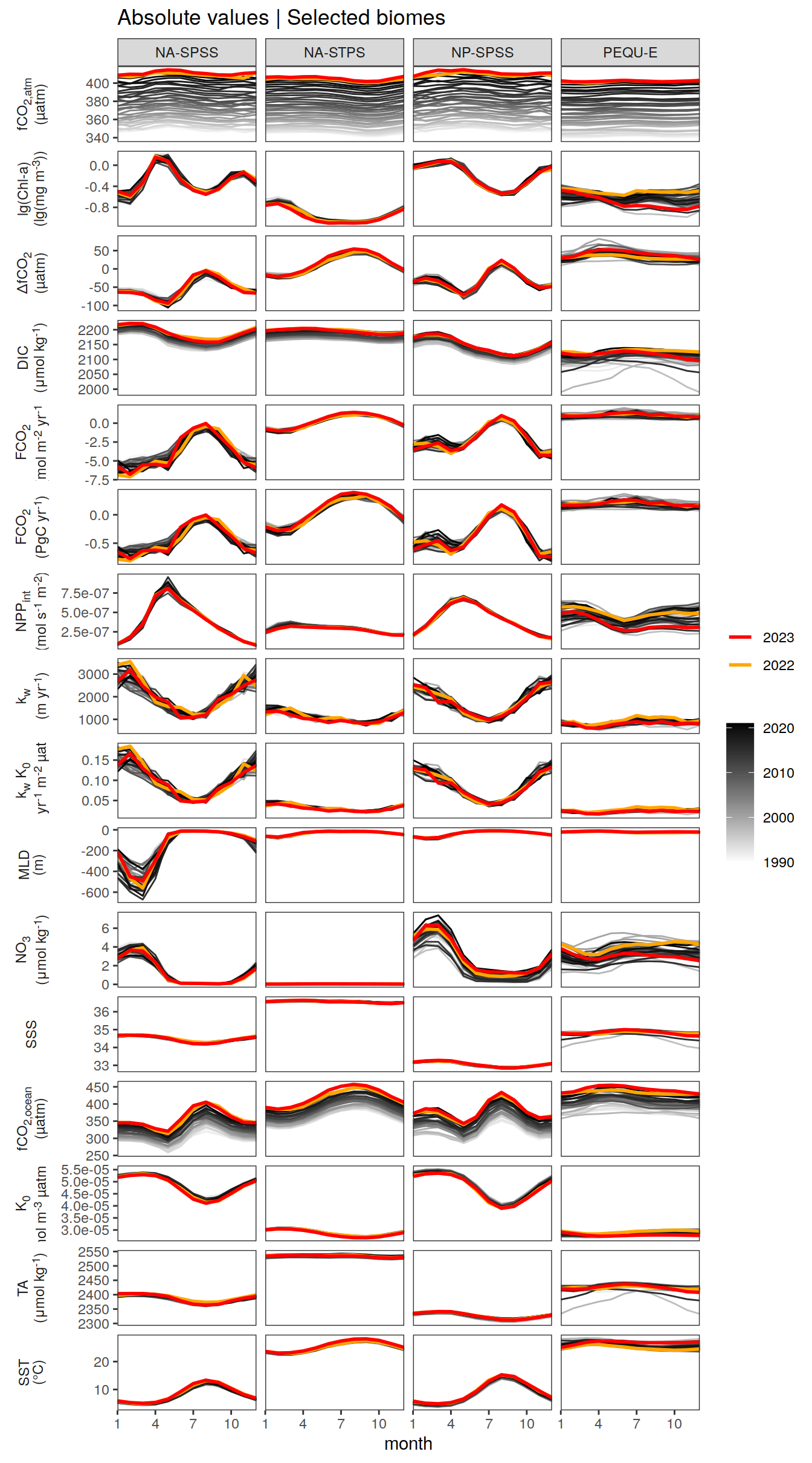
Regional means and integrals
The following plots show regionally averaged (or integrated) values of each variable as provided through the pCO2 product, as well as the anomalies from the prediction of a linear/quadratic fit.
Anomalies are first presented relative to the predicted annual mean of each year, hence preserving the seasonality. Furthermore, anomalies are presented relative to the predicted monthly mean values, such that the mean seasonality is removed.
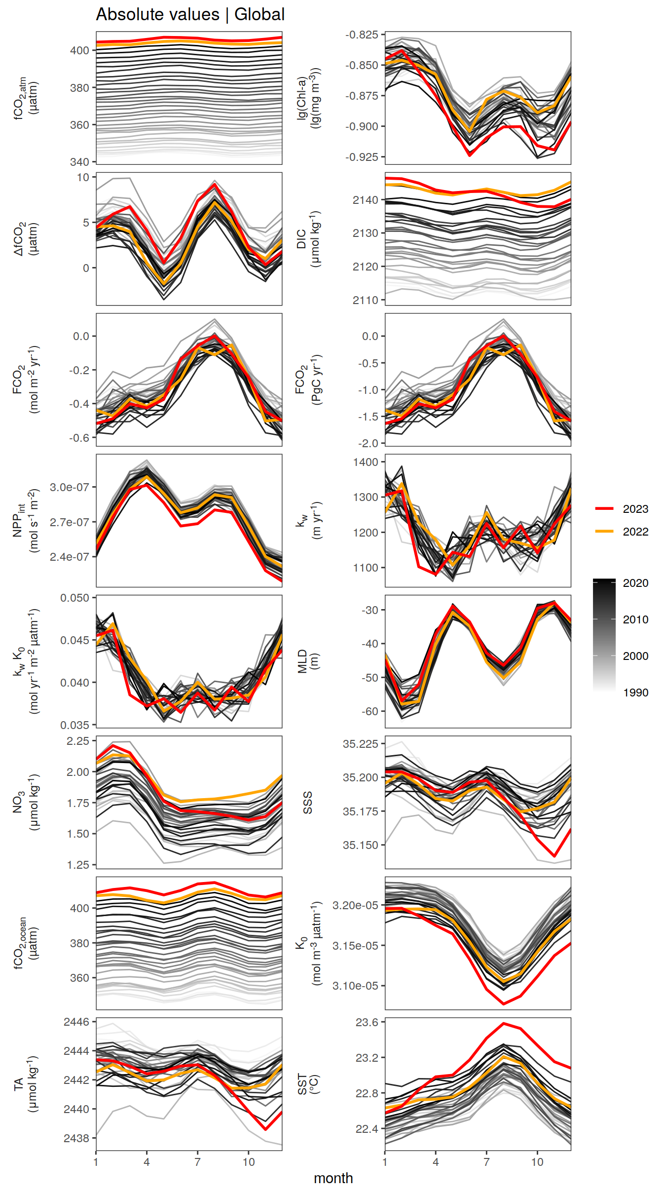
2023 absolute values
Global
fig.height <- pco2_product_monthly %>%
  distinct(name) %>%
  nrow()

fig.height <- (fig.height + 2) * 0.1
pco2_product_monthly %>%
filter(biome %in% "Global") %>%
ggplot(aes(month, value, group = as.factor(year))) +
geom_path(data = . %>% filter(!between(year, 2023-1, 2023)),
aes(col = year)) +
scale_color_grayC() +
new_scale_color() +
geom_path(data = . %>% filter(between(year, 2023-1, 2023)),
aes(col = as.factor(year)),
linewidth = 1) +
scale_color_manual(values = c("orange", "red"),
guide = guide_legend(reverse = TRUE,
order = 1)) +
scale_x_continuous(breaks = seq(1, 12, 3), expand = c(0, 0)) +
labs(title = "Absolute values | Global") +
facet_wrap(name ~ .,
scales = "free_y",
labeller = labeller(name = x_axis_labels),
strip.position = "left",
ncol = 2) +
theme(
strip.text.y.left = element_markdown(),
strip.placement = "outside",
strip.background.y = element_blank(),
legend.title = element_blank(),
axis.title.y = element_blank()
)
| Version | Author | Date |
|---|---|---|
| 054921b | jens-daniel-mueller | 2024-05-23 |
| 38f6f6e | jens-daniel-mueller | 2024-05-22 |
| be285dc | jens-daniel-mueller | 2024-05-21 |
| 51df30d | jens-daniel-mueller | 2024-05-15 |
| 009791f | jens-daniel-mueller | 2024-05-14 |
| 3b5d16b | jens-daniel-mueller | 2024-05-13 |
| fb21e78 | jens-daniel-mueller | 2024-05-08 |
| c7897dc | jens-daniel-mueller | 2024-05-08 |
Selected biomes
pco2_product_monthly %>%
  filter(biome %in% key_biomes) %>%
  ggplot(aes(month, value, group = as.factor(year))) +
  geom_path(data = . %>% filter(!between(year, 2023-1, 2023)),
            aes(col = year)) +
  scale_color_grayC() +
  new_scale_color() +
  geom_path(data = . %>% filter(between(year, 2023-1, 2023)),
            aes(col = as.factor(year)),
            linewidth = 1) +
  scale_color_manual(values = c("orange", "red"),
                     guide = guide_legend(reverse = TRUE,
                                          order = 1)) +
  scale_x_continuous(breaks = seq(1, 12, 3), expand = c(0, 0)) +
  labs(title = "Absolute values | Selected biomes") +
  facet_grid(name ~ biome,
             scales = "free_y",
             labeller = labeller(name = x_axis_labels),
             switch = "y") +
  theme(
    strip.text.y.left = element_markdown(),
    strip.placement = "outside",
    strip.background.y = element_blank(),
    legend.title = element_blank(),
    axis.title.y = element_blank()
  )
| Version | Author | Date |
|---|---|---|
| 054921b | jens-daniel-mueller | 2024-05-23 |
| 38f6f6e | jens-daniel-mueller | 2024-05-22 |
| be285dc | jens-daniel-mueller | 2024-05-21 |
| 51df30d | jens-daniel-mueller | 2024-05-15 |
| 009791f | jens-daniel-mueller | 2024-05-14 |
| 3b5d16b | jens-daniel-mueller | 2024-05-13 |
| fb21e78 | jens-daniel-mueller | 2024-05-08 |
| c7897dc | jens-daniel-mueller | 2024-05-08 |
pco2_product_monthly %>%
  filter(biome %in% key_biomes) %>%
  group_split(biome) %>%
  # head(1) %>%
  map(
    ~ ggplot(data = .x,
             aes(month, value, group = as.factor(year))) +
      geom_path(data = . %>% filter(!between(year, 2023-1, 2023)),
                aes(col = year)) +
      scale_color_grayC() +
      new_scale_color() +
      geom_path(
        data = . %>% filter(between(year, 2023-1, 2023)),
        aes(col = as.factor(year)),
        linewidth = 1
      ) +
      scale_color_manual(
        values = c("orange", "red"),
        guide = guide_legend(reverse = TRUE,
                             order = 1)
      ) +
      scale_x_continuous(breaks = seq(1, 12, 3), expand = c(0, 0)) +
  labs(title = paste("Absolute values |", .x$biome)) +
  facet_wrap(name ~ .,
             scales = "free_y",
             labeller = labeller(name = x_axis_labels),
             strip.position = "left",
             ncol = 2) +
  theme(
    strip.text.y.left = element_markdown(),
    strip.placement = "outside",
    strip.background.y = element_blank(),
    legend.title = element_blank(),
    axis.title.y = element_blank()
  )
  )
[[1]]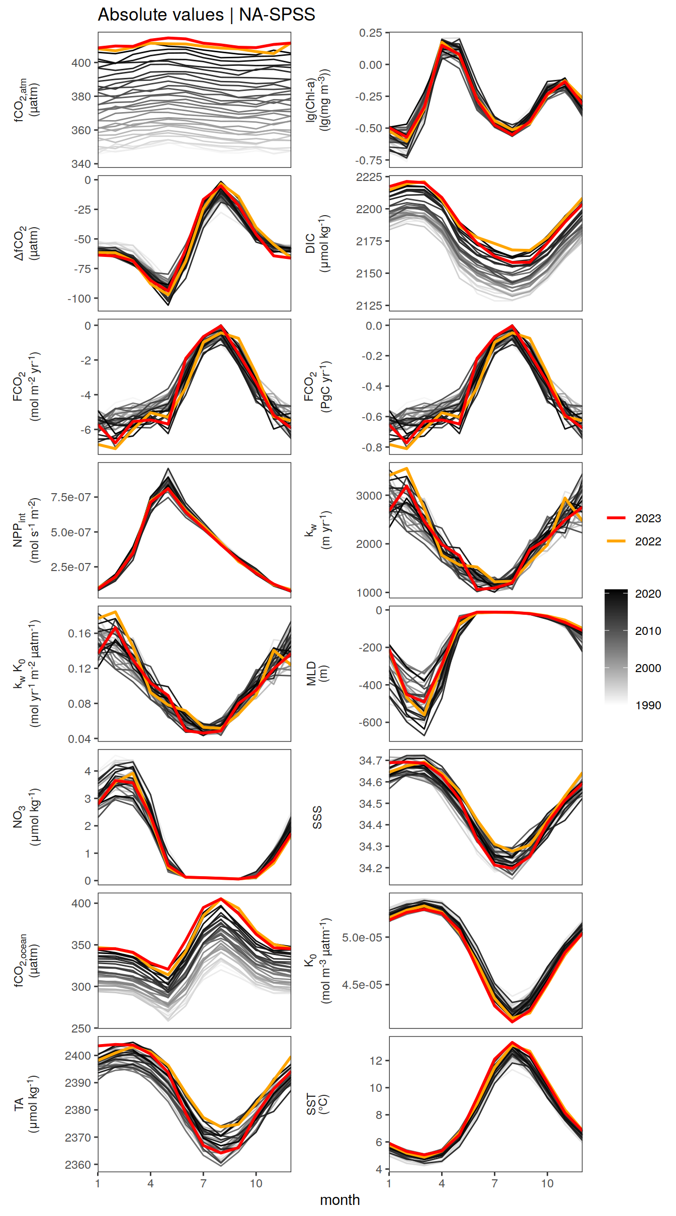
[[2]]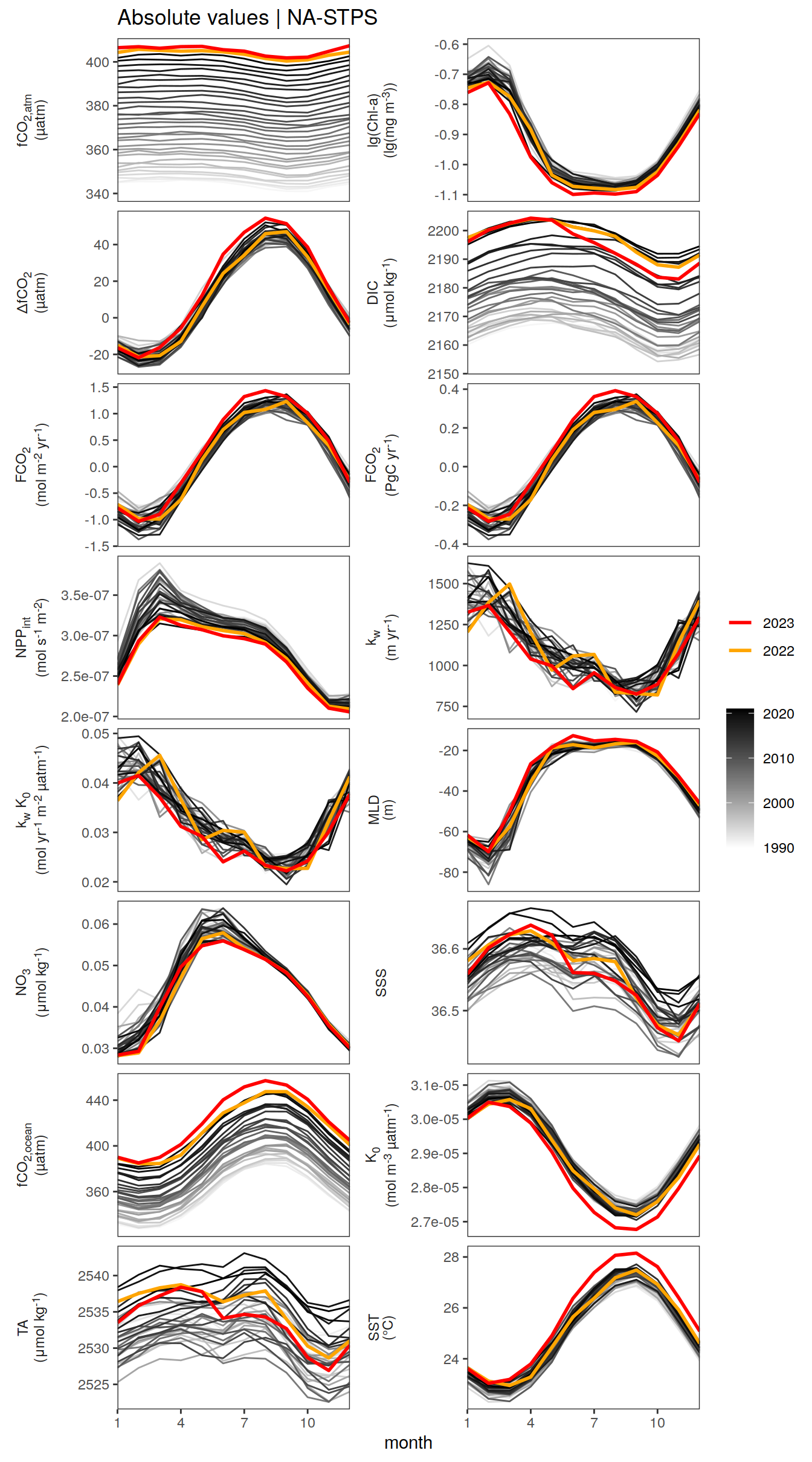
[[3]]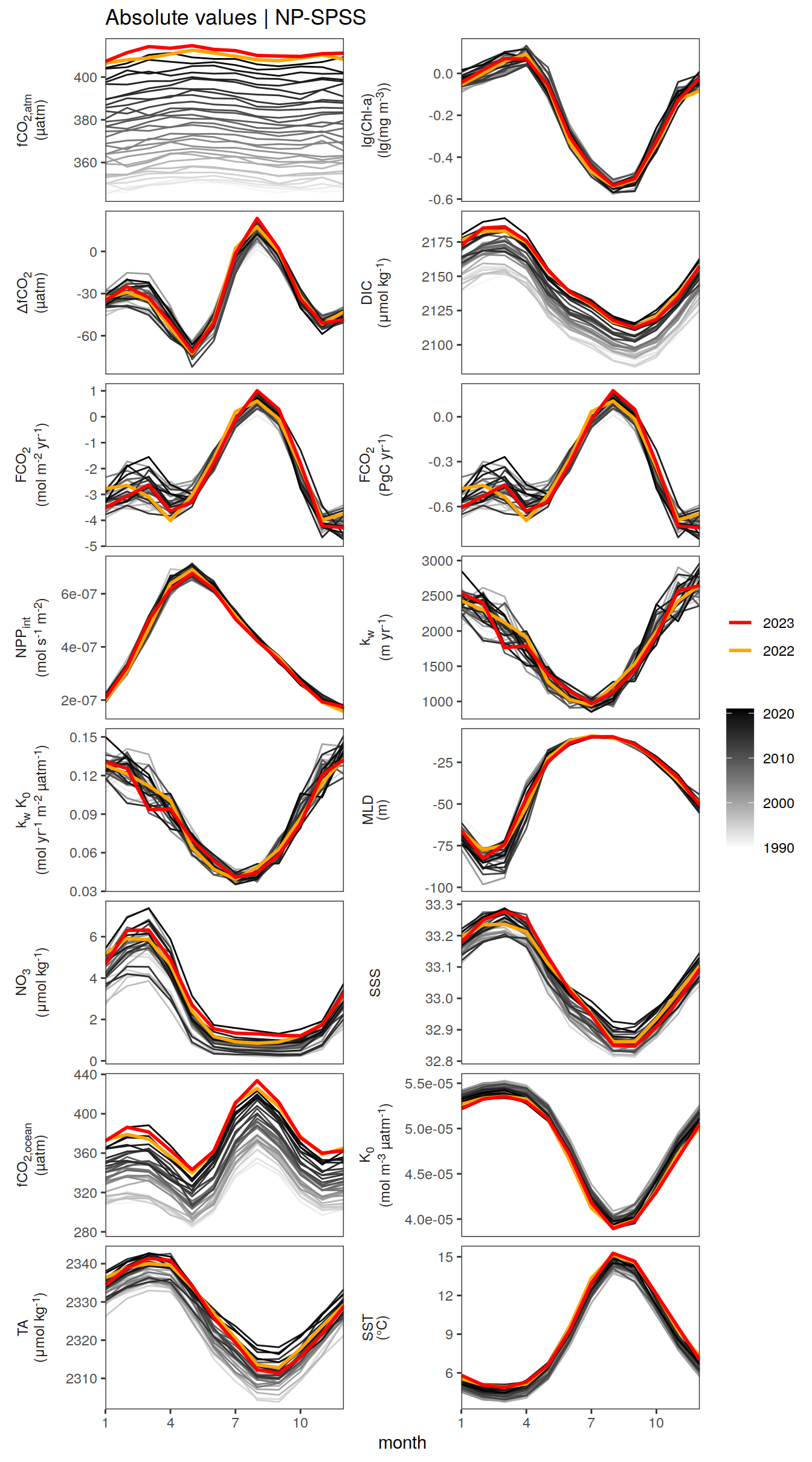
[[4]]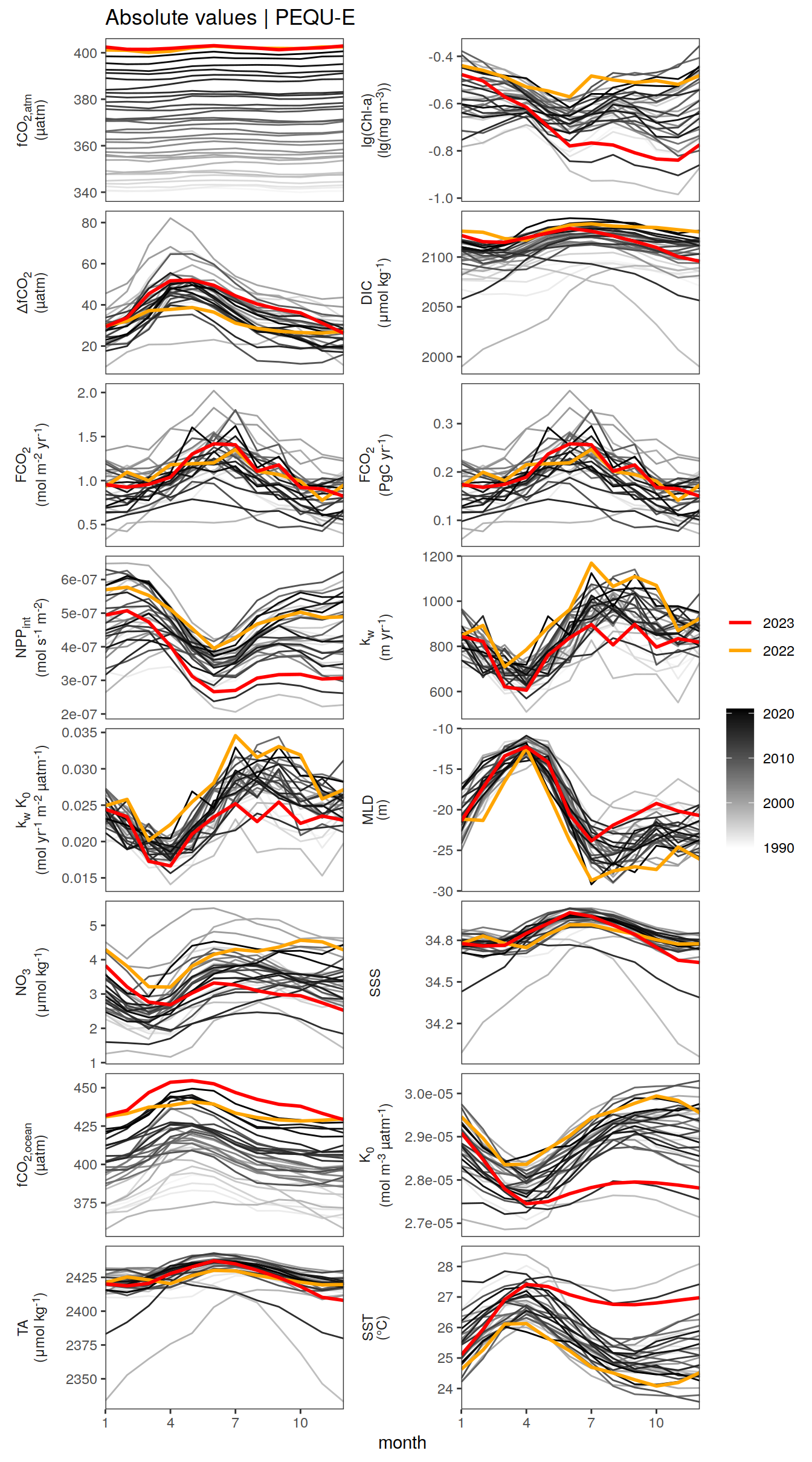
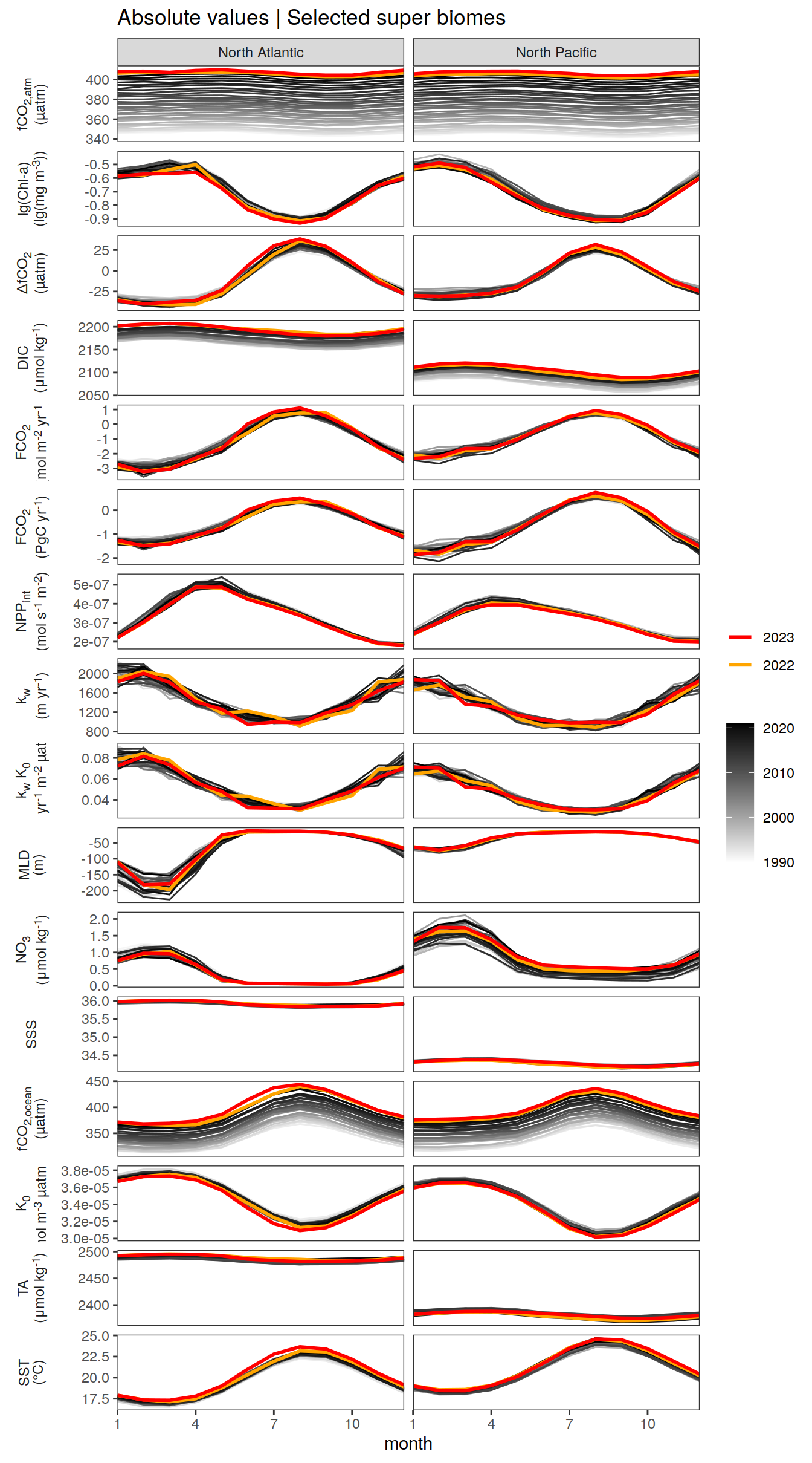
Super biomes
pco2_product_monthly %>%
  filter(biome %in% super_biomes) %>%
  ggplot(aes(month, value, group = as.factor(year))) +
  geom_path(data = . %>% filter(!between(year, 2023-1, 2023)),
            aes(col = year)) +
  scale_color_grayC() +
  new_scale_color() +
  geom_path(data = . %>% filter(between(year, 2023-1, 2023)),
            aes(col = as.factor(year)),
            linewidth = 1) +
  scale_color_manual(values = c("orange", "red"),
                     guide = guide_legend(reverse = TRUE,
                                          order = 1)) +
  scale_x_continuous(breaks = seq(1, 12, 3), expand = c(0, 0)) +
  labs(title = "Absolute values | Selected super biomes") +
  facet_grid(name ~ biome,
             scales = "free_y",
             labeller = labeller(name = x_axis_labels),
             switch = "y") +
  theme(
    strip.text.y.left = element_markdown(),
    strip.placement = "outside",
    strip.background.y = element_blank(),
    legend.title = element_blank(),
    axis.title.y = element_blank()
  )
| Version | Author | Date |
|---|---|---|
| 054921b | jens-daniel-mueller | 2024-05-23 |
| 38f6f6e | jens-daniel-mueller | 2024-05-22 |
| be285dc | jens-daniel-mueller | 2024-05-21 |
| 51df30d | jens-daniel-mueller | 2024-05-15 |
| 009791f | jens-daniel-mueller | 2024-05-14 |
| 3b5d16b | jens-daniel-mueller | 2024-05-13 |
| fb21e78 | jens-daniel-mueller | 2024-05-08 |
| c7897dc | jens-daniel-mueller | 2024-05-08 |
pco2_product_monthly %>%
  filter(biome %in% super_biomes) %>%
  group_split(biome) %>%
  # head(1) %>%
  map(
    ~ ggplot(data = .x,
             aes(month, value, group = as.factor(year))) +
      geom_path(data = . %>% filter(!between(year, 2023-1, 2023)),
                aes(col = year)) +
      scale_color_grayC() +
      new_scale_color() +
      geom_path(
        data = . %>% filter(between(year, 2023-1, 2023)),
        aes(col = as.factor(year)),
        linewidth = 1
      ) +
      scale_color_manual(
        values = c("orange", "red"),
        guide = guide_legend(reverse = TRUE,
                             order = 1)
      ) +
      scale_x_continuous(breaks = seq(1, 12, 3), expand = c(0, 0)) +
  labs(title = paste("Absolute values |", .x$biome)) +
  facet_wrap(name ~ .,
             scales = "free_y",
             labeller = labeller(name = x_axis_labels),
             strip.position = "left",
             ncol = 2) +
  theme(
    strip.text.y.left = element_markdown(),
    strip.placement = "outside",
    strip.background.y = element_blank(),
    legend.title = element_blank(),
    axis.title.y = element_blank()
  )
  )
[[1]]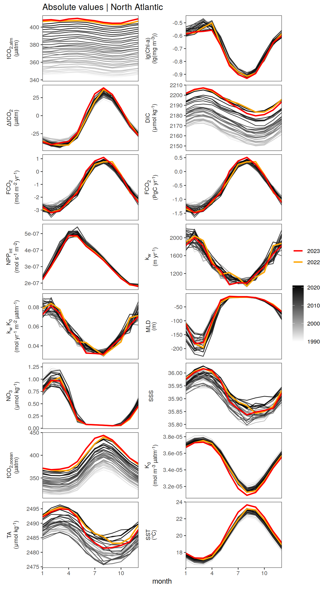
[[2]]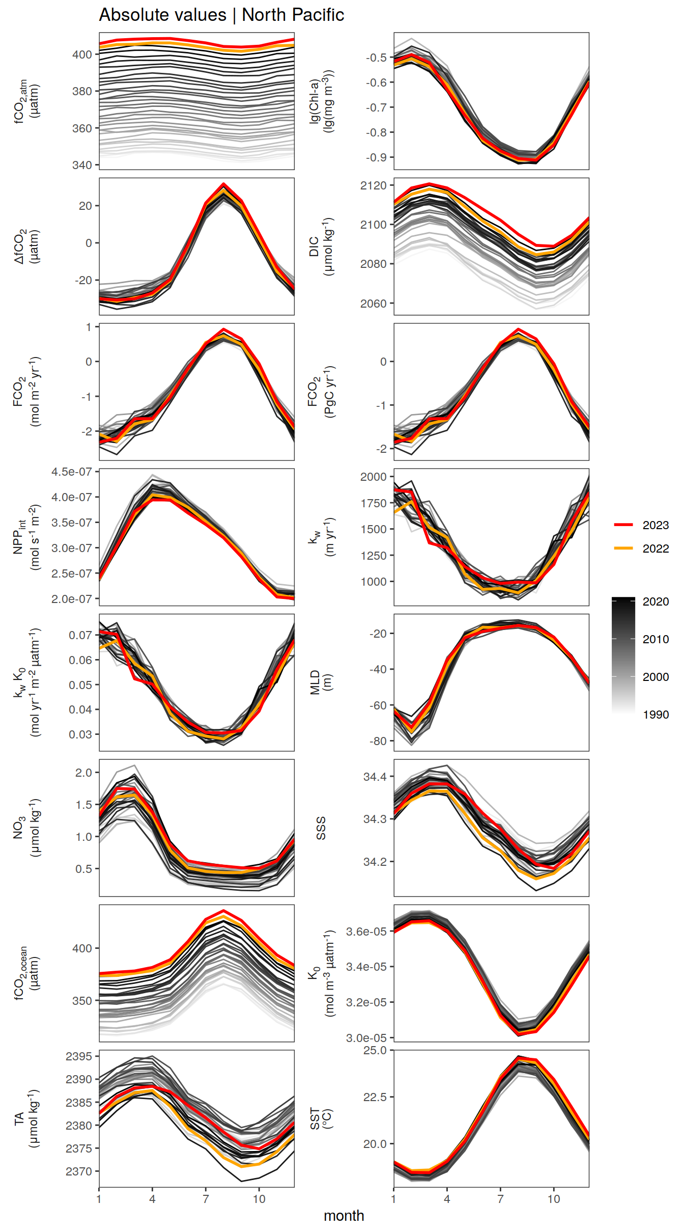
2023 anomalies
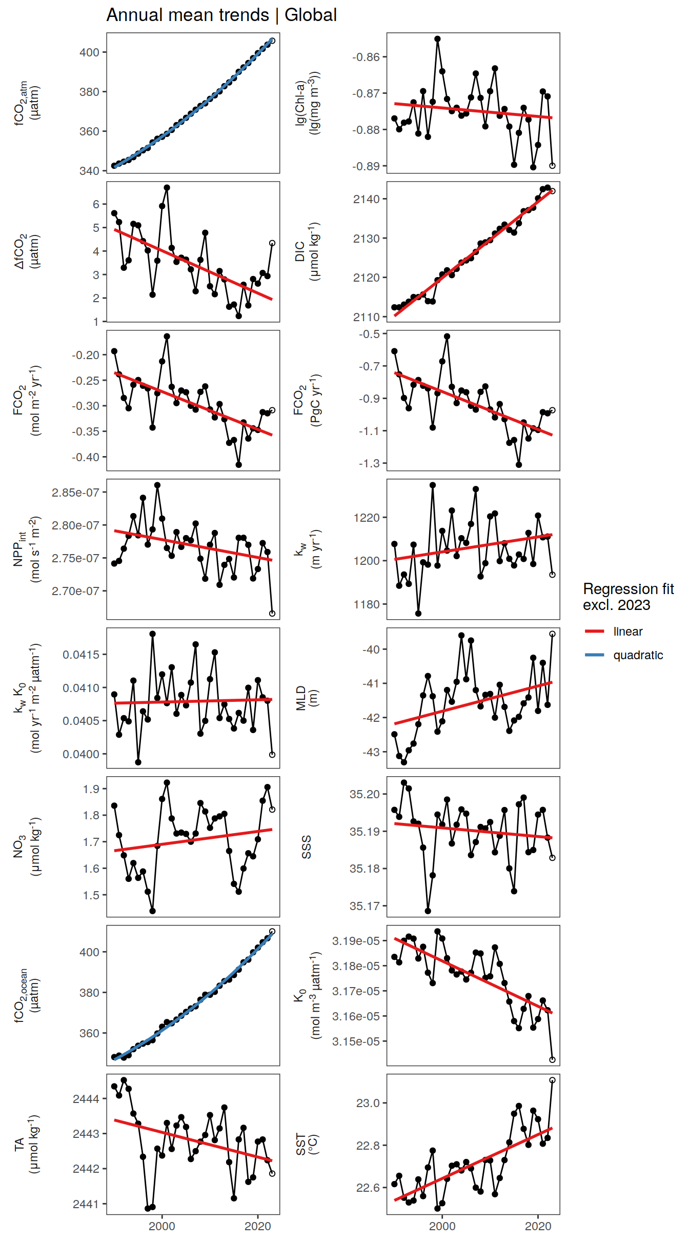
Annual mean trends
pco2_product_annual <-
  pco2_product_monthly %>%
  group_by(year, biome, name) %>%
  summarise(value = mean(value)) %>%
  ungroup()

pco2_product_annual %>%
  filter(biome %in% "Global") %>%
  ggplot(aes(year, value)) +
  geom_path() +
  geom_point(data = . %>% filter(year != 2023)) +
  geom_point(data = . %>% filter(year == 2023),
             shape = 1) +
  geom_smooth(data = . %>% filter(year != 2023,
                                  !(name %in% name_quadratic_fit)),
              method = "lm",
              fullrange = TRUE,
              aes(col = "linear"),
              se = FALSE) +
  geom_smooth(data = . %>% filter(year != 2023,
                                  name %in% name_quadratic_fit),
              method = "lm",
              fullrange = TRUE,
              formula = y ~ x + I(x^2),
              aes(col = "quadratic"),
              se = FALSE) +
  scale_color_brewer(
    palette = "Set1",
    name = paste("Regression fit\nexcl.", 2023)) +
  scale_x_continuous(breaks = seq(1980, 2020, 20)) +
  labs(title = "Annual mean trends | Global") +
  facet_wrap(name ~ .,
             scales = "free_y",
             labeller = labeller(name = x_axis_labels),
             strip.position = "left",
             ncol = 2) +
  theme(
    strip.text.y.left = element_markdown(),
    strip.placement = "outside",
    strip.background.y = element_blank(),
    axis.title = element_blank()
  )
| Version | Author | Date |
|---|---|---|
| 054921b | jens-daniel-mueller | 2024-05-23 |
| 38f6f6e | jens-daniel-mueller | 2024-05-22 |
| be285dc | jens-daniel-mueller | 2024-05-21 |
| 51df30d | jens-daniel-mueller | 2024-05-15 |
| 009791f | jens-daniel-mueller | 2024-05-14 |
| 3b5d16b | jens-daniel-mueller | 2024-05-13 |
| fb21e78 | jens-daniel-mueller | 2024-05-08 |
| c7897dc | jens-daniel-mueller | 2024-05-08 |
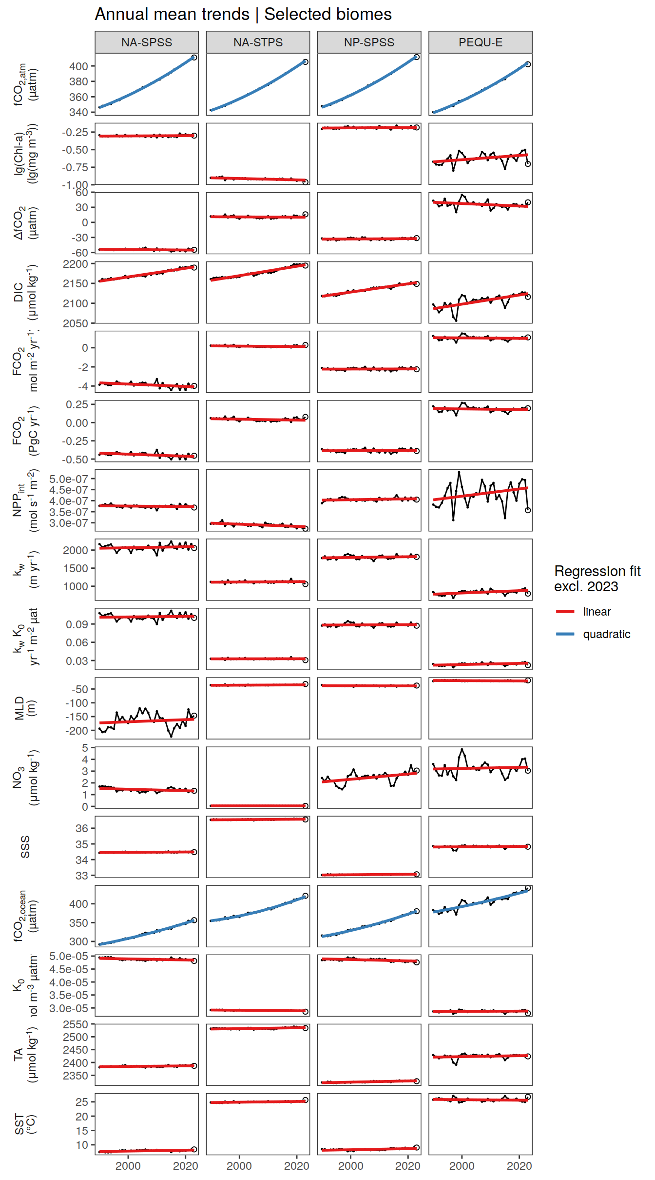
pco2_product_annual %>%
  filter(biome %in% key_biomes) %>%
  ggplot(aes(year, value)) +
  geom_path() +
  geom_point(data = . %>% filter(year != 2023),
             size = 0.2) +
  geom_point(data = . %>% filter(year == 2023),
             shape = 1) +
  geom_smooth(data = . %>% filter(year != 2023,
                                  !(name %in% name_quadratic_fit)),
              method = "lm",
              fullrange = TRUE,
              aes(col = "linear"),
              se = FALSE) +
  geom_smooth(data = . %>% filter(year != 2023,
                                  name %in% name_quadratic_fit),
              method = "lm",
              fullrange = TRUE,
              formula = y ~ x + I(x^2),
              aes(col = "quadratic"),
              se = FALSE) +
  scale_color_brewer(
    palette = "Set1",
    name = paste("Regression fit\nexcl.", 2023)) +
  scale_x_continuous(breaks = seq(1980, 2020, 20)) +
  labs(title = "Annual mean trends | Selected biomes") +
  facet_grid(name ~ biome,
             scales = "free_y",
             labeller = labeller(name = x_axis_labels),
             switch = "y") +
  theme(
    strip.text.y.left = element_markdown(),
    strip.placement = "outside",
    strip.background.y = element_blank(),
    axis.title = element_blank()
  )
| Version | Author | Date |
|---|---|---|
| 054921b | jens-daniel-mueller | 2024-05-23 |
| 38f6f6e | jens-daniel-mueller | 2024-05-22 |
| be285dc | jens-daniel-mueller | 2024-05-21 |
| 51df30d | jens-daniel-mueller | 2024-05-15 |
| 009791f | jens-daniel-mueller | 2024-05-14 |
| 3b5d16b | jens-daniel-mueller | 2024-05-13 |
| fb21e78 | jens-daniel-mueller | 2024-05-08 |
| c7897dc | jens-daniel-mueller | 2024-05-08 |
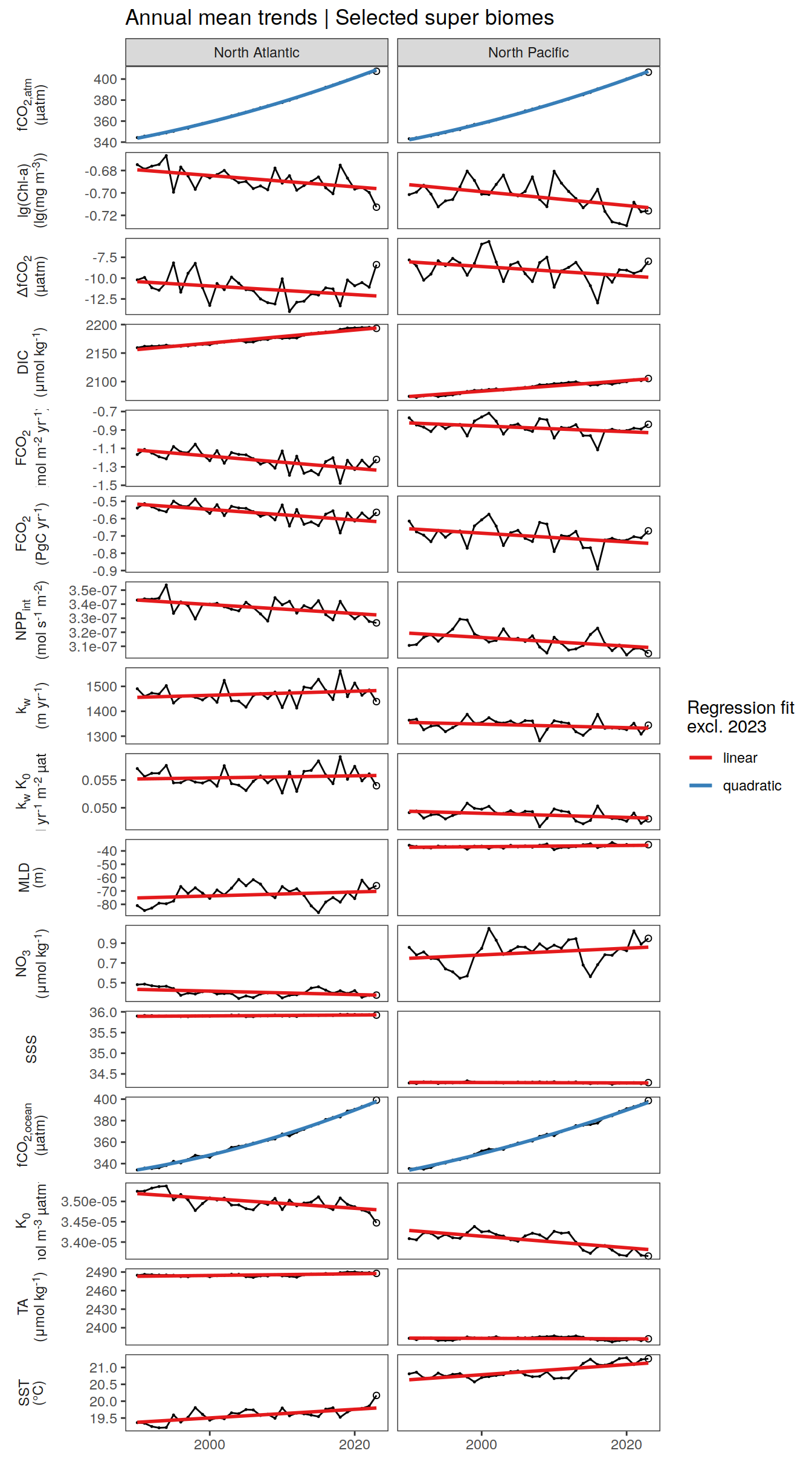
pco2_product_annual %>%
  filter(biome %in% super_biomes) %>%
  ggplot(aes(year, value)) +
  geom_path() +
  geom_point(data = . %>% filter(year != 2023),
             size = 0.2) +
  geom_point(data = . %>% filter(year == 2023),
             shape = 1) +
  geom_smooth(data = . %>% filter(year != 2023,
                                  !(name %in% name_quadratic_fit)),
              method = "lm",
              fullrange = TRUE,
              aes(col = "linear"),
              se = FALSE) +
  geom_smooth(data = . %>% filter(year != 2023,
                                  name %in% name_quadratic_fit),
              method = "lm",
              fullrange = TRUE,
              formula = y ~ x + I(x^2),
              aes(col = "quadratic"),
              se = FALSE) +
  scale_color_brewer(
    palette = "Set1",
    name = paste("Regression fit\nexcl.", 2023)) +
  scale_x_continuous(breaks = seq(1980, 2020, 20)) +
  labs(title = "Annual mean trends | Selected super biomes") +
  facet_grid(name ~ biome,
             scales = "free_y",
             labeller = labeller(name = x_axis_labels),
             switch = "y") +
  theme(
    strip.text.y.left = element_markdown(),
    strip.placement = "outside",
    strip.background.y = element_blank(),
    axis.title = element_blank()
  )
| Version | Author | Date |
|---|---|---|
| 054921b | jens-daniel-mueller | 2024-05-23 |
| 38f6f6e | jens-daniel-mueller | 2024-05-22 |
| be285dc | jens-daniel-mueller | 2024-05-21 |
| 51df30d | jens-daniel-mueller | 2024-05-15 |
| 009791f | jens-daniel-mueller | 2024-05-14 |
| 3b5d16b | jens-daniel-mueller | 2024-05-13 |
| fb21e78 | jens-daniel-mueller | 2024-05-08 |
| c7897dc | jens-daniel-mueller | 2024-05-08 |
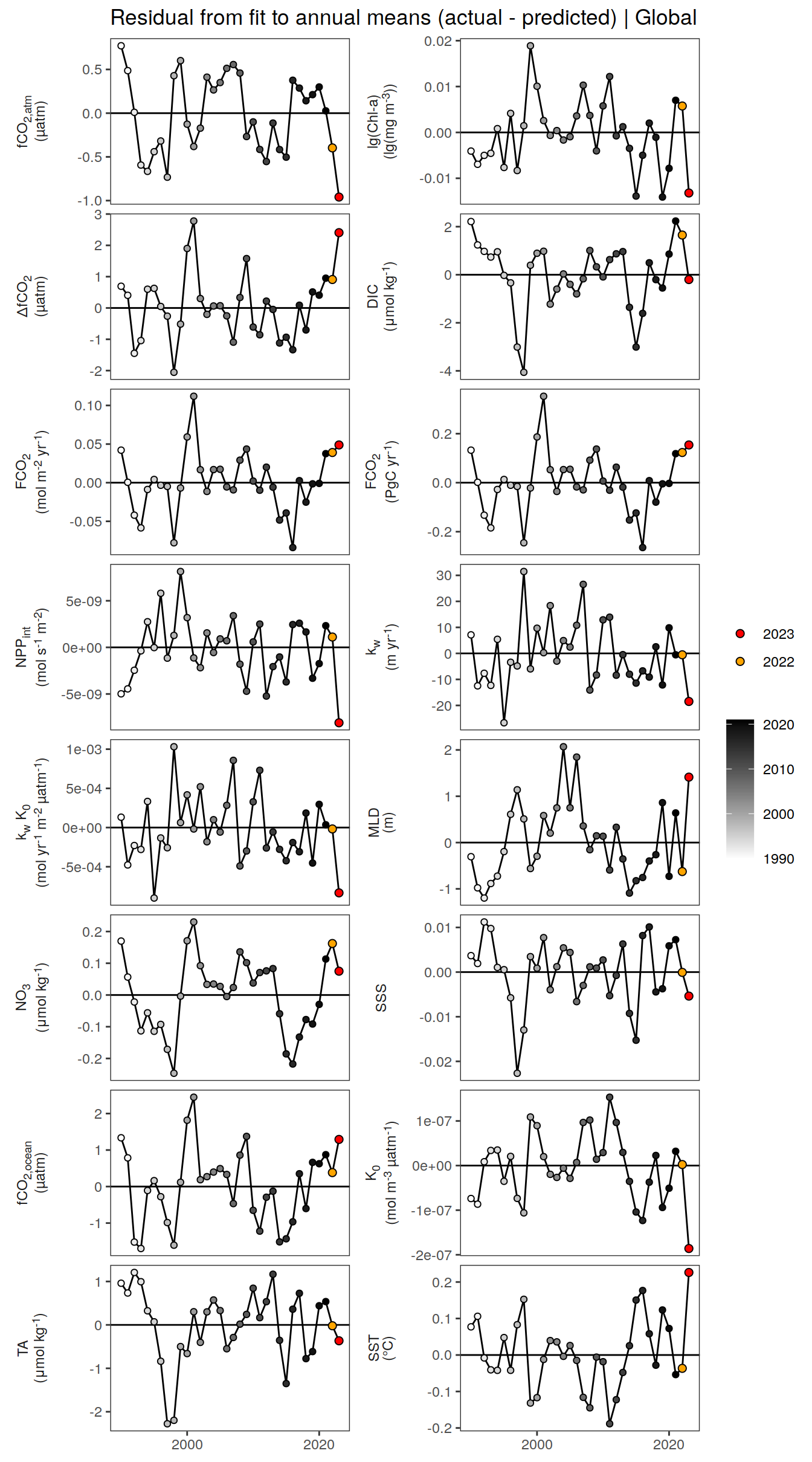
pco2_product_annual_regression <-
  pco2_product_annual %>%
  anomaly_determination(biome)


pco2_product_annual_regression %>%
  filter(biome %in% "Global") %>%
  ggplot(aes(year, resid)) +
  geom_hline(yintercept = 0) +
  geom_path() +
  geom_point(data = . %>% filter(!between(year, 2023-1, 2023)),
             aes(fill = year),
             shape = 21) +
  scale_fill_grayC() +
  new_scale_fill() +
  geom_point(data = . %>% filter(between(year, 2023-1, 2023)),
             aes(fill = as.factor(year)),
             shape = 21, size = 2)  +
  scale_fill_manual(values = c("orange", "red"),
                     guide = guide_legend(reverse = TRUE,
                                          order = 1)) +
  scale_x_continuous(breaks = seq(1980, 2020, 20)) +
  labs(title = "Residual from fit to annual means (actual - predicted) | Global") +
  facet_wrap(name ~ .,
             scales = "free_y",
             labeller = labeller(name = x_axis_labels),
             strip.position = "left",
             ncol = 2) +
  theme(
    strip.text.y.left = element_markdown(),
    strip.placement = "outside",
    strip.background.y = element_blank(),
    axis.title = element_blank(),
    legend.title = element_blank()
  )
| Version | Author | Date |
|---|---|---|
| 054921b | jens-daniel-mueller | 2024-05-23 |
| 38f6f6e | jens-daniel-mueller | 2024-05-22 |
| be285dc | jens-daniel-mueller | 2024-05-21 |
| 51df30d | jens-daniel-mueller | 2024-05-15 |
| 009791f | jens-daniel-mueller | 2024-05-14 |
| 3b5d16b | jens-daniel-mueller | 2024-05-13 |
| fb21e78 | jens-daniel-mueller | 2024-05-08 |
| c7897dc | jens-daniel-mueller | 2024-05-08 |
pco2_product_annual_regression %>%
  filter(biome %in% key_biomes) %>%
  ggplot(aes(year, resid)) +
  geom_hline(yintercept = 0) +
  geom_path() +
  geom_point(data = . %>% filter(!between(year, 2023-1, 2023)),
             aes(fill = year),
             shape = 21) +
  scale_fill_grayC() +
  new_scale_fill() +
  geom_point(data = . %>% filter(between(year, 2023-1, 2023)),
             aes(fill = as.factor(year)),
             shape = 21, size = 2)  +
  scale_fill_manual(values = c("orange", "red"),
                     guide = guide_legend(reverse = TRUE,
                                          order = 1)) +
  scale_x_continuous(breaks = seq(1980, 2020, 20)) +
  labs(title = "Residual from fit to annual means (actual - predicted) | Selected biomes") +
  facet_grid(name ~ biome,
             scales = "free_y",
             labeller = labeller(name = x_axis_labels),
             switch = "y") +
  theme(
    strip.text.y.left = element_markdown(),
    strip.placement = "outside",
    strip.background.y = element_blank(),
    axis.title = element_blank(),
    legend.title = element_blank()
  )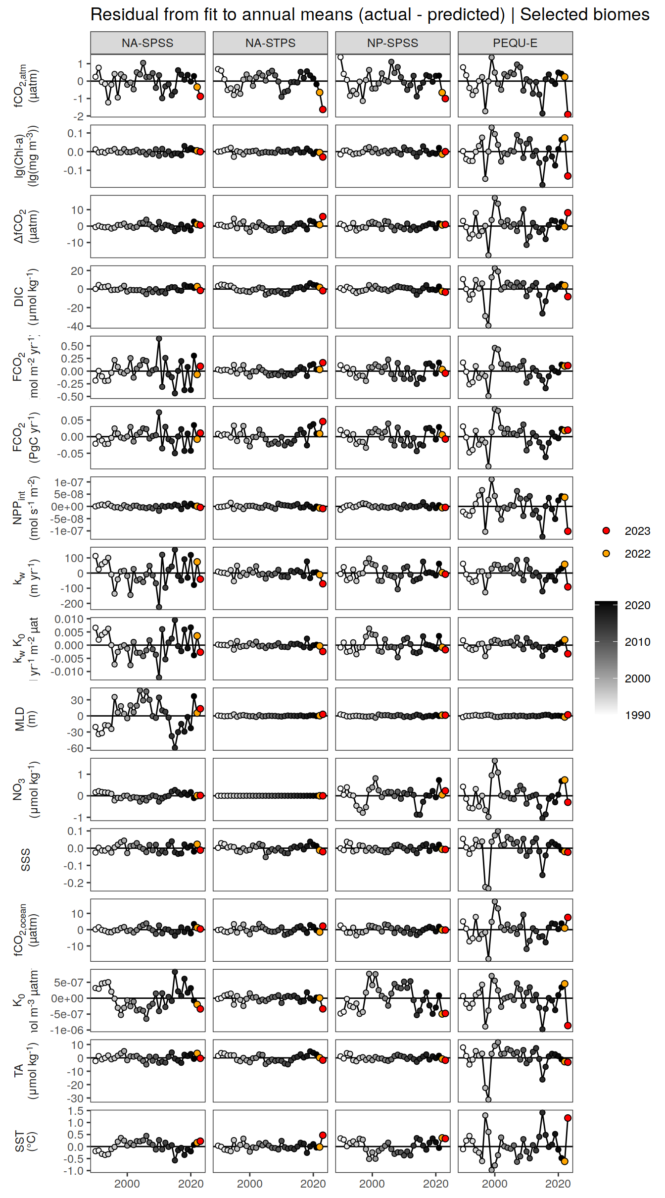
| Version | Author | Date |
|---|---|---|
| 054921b | jens-daniel-mueller | 2024-05-23 |
| 38f6f6e | jens-daniel-mueller | 2024-05-22 |
| be285dc | jens-daniel-mueller | 2024-05-21 |
| 51df30d | jens-daniel-mueller | 2024-05-15 |
| 009791f | jens-daniel-mueller | 2024-05-14 |
| 3b5d16b | jens-daniel-mueller | 2024-05-13 |
| fb21e78 | jens-daniel-mueller | 2024-05-08 |
| c7897dc | jens-daniel-mueller | 2024-05-08 |
pco2_product_annual_regression %>%
  filter(biome %in% super_biomes) %>%
  ggplot(aes(year, resid)) +
  geom_hline(yintercept = 0) +
  geom_path() +
  geom_point(data = . %>% filter(!between(year, 2023-1, 2023)),
             aes(fill = year),
             shape = 21) +
  scale_fill_grayC() +
  new_scale_fill() +
  geom_point(data = . %>% filter(between(year, 2023-1, 2023)),
             aes(fill = as.factor(year)),
             shape = 21, size = 2)  +
  scale_fill_manual(values = c("orange", "red"),
                     guide = guide_legend(reverse = TRUE,
                                          order = 1)) +
  scale_x_continuous(breaks = seq(1980, 2020, 20)) +
  labs(title = "Residual from fit to annual means (actual - predicted) | Selected super biomes") +
  facet_grid(name ~ biome,
             scales = "free_y",
             labeller = labeller(name = x_axis_labels),
             switch = "y") +
  theme(
    strip.text.y.left = element_markdown(),
    strip.placement = "outside",
    strip.background.y = element_blank(),
    axis.title = element_blank(),
    legend.title = element_blank()
  )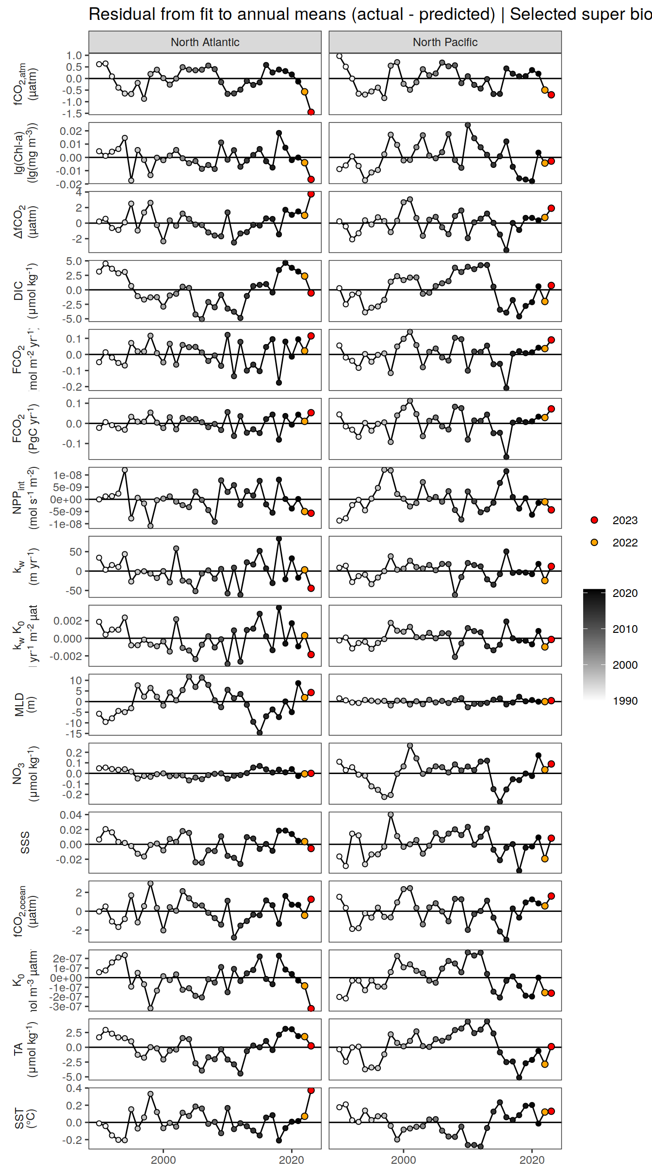
| Version | Author | Date |
|---|---|---|
| 054921b | jens-daniel-mueller | 2024-05-23 |
| 38f6f6e | jens-daniel-mueller | 2024-05-22 |
| be285dc | jens-daniel-mueller | 2024-05-21 |
| 51df30d | jens-daniel-mueller | 2024-05-15 |
| 009791f | jens-daniel-mueller | 2024-05-14 |
| 3b5d16b | jens-daniel-mueller | 2024-05-13 |
| fb21e78 | jens-daniel-mueller | 2024-05-08 |
| c7897dc | jens-daniel-mueller | 2024-05-08 |
pco2_product_annual_regression %>%
  filter(biome != "global") %>%
  ggplot(aes(biome, resid)) +
  geom_hline(yintercept = 0) +
  geom_jitter(data = . %>% filter(!between(year, 2023-1, 2023)),
             aes(fill = year),
             shape = 21, width = 0.2) +
  scale_fill_grayC() +
  new_scale_fill() +
  geom_point(data = . %>% filter(between(year, 2023-1, 2023)),
             aes(fill = as.factor(year)),
             shape = 21, size = 2)  +
  scale_fill_manual(values = c("orange", "red"),
                     guide = guide_legend(reverse = TRUE,
                                          order = 1)) +
  labs(title = "Residual from fit to annual means (actual - predicted) | All biomes") +
  facet_grid(name ~ .,
             scales = "free_y",
             labeller = labeller(name = x_axis_labels),
             switch = "y") +
  theme(
    strip.text.y.left = element_markdown(),
    strip.placement = "outside",
    strip.background.y = element_blank(),
    axis.title = element_blank(),
    legend.title = element_blank(),
        axis.text.x = element_text(angle = 90, vjust = 0.5, hjust=1)
  )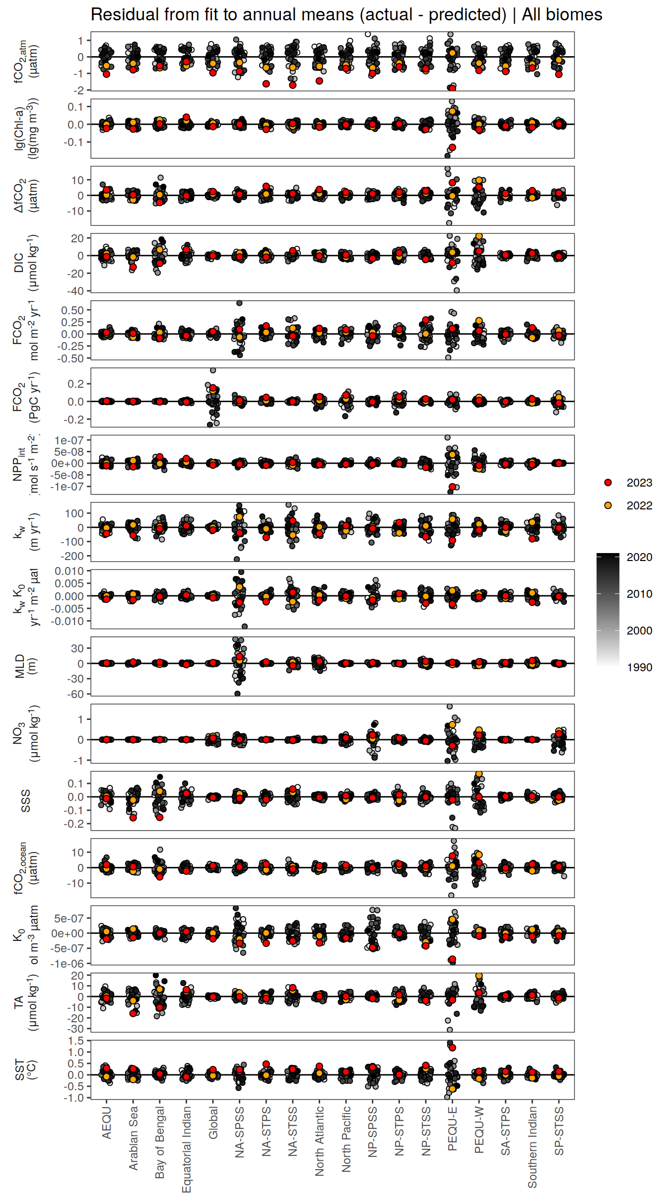
| Version | Author | Date |
|---|---|---|
| 054921b | jens-daniel-mueller | 2024-05-23 |
| 38f6f6e | jens-daniel-mueller | 2024-05-22 |
| be285dc | jens-daniel-mueller | 2024-05-21 |
| 51df30d | jens-daniel-mueller | 2024-05-15 |
| 009791f | jens-daniel-mueller | 2024-05-14 |
| 3b5d16b | jens-daniel-mueller | 2024-05-13 |
| fb21e78 | jens-daniel-mueller | 2024-05-08 |
| c7897dc | jens-daniel-mueller | 2024-05-08 |
pco2_product_annual_regression %>%
  write_csv(paste0("../data/","FESOM-REcoM","_","2023","_biome_annual_regression.csv"))
pco2_product_annual_detrended <-
full_join(pco2_product_monthly,
pco2_product_annual_regression %>% select(-c(value, resid))) %>%
mutate(resid = value - fit)
pco2_product_annual_detrended %>%
filter(biome %in% "Global") %>%
ggplot(aes(month, resid, group = as.factor(year))) +
geom_path(data = . %>% filter(!between(year, 2023-1, 2023)),
aes(col = year)) +
scale_color_grayC() +
new_scale_color() +
geom_path(data = . %>% filter(between(year, 2023-1, 2023)),
aes(col = as.factor(year)),
linewidth = 1) +
scale_color_manual(values = c("orange", "red"),
guide = guide_legend(reverse = TRUE,
order = 1)) +
scale_x_continuous(breaks = seq(1, 12, 3), expand = c(0, 0)) +
labs(title = "Anomalies from predicted annual mean | Global") +
facet_wrap(name ~ .,
scales = "free_y",
labeller = labeller(name = x_axis_labels),
strip.position = "left",
ncol = 2) +
theme(
strip.text.y.left = element_markdown(),
strip.placement = "outside",
strip.background.y = element_blank(),
axis.title.y = element_blank(),
legend.title = element_blank()
)
| Version | Author | Date |
|---|---|---|
| 054921b | jens-daniel-mueller | 2024-05-23 |
| 38f6f6e | jens-daniel-mueller | 2024-05-22 |
| be285dc | jens-daniel-mueller | 2024-05-21 |
| 51df30d | jens-daniel-mueller | 2024-05-15 |
| 009791f | jens-daniel-mueller | 2024-05-14 |
| 3b5d16b | jens-daniel-mueller | 2024-05-13 |
| fb21e78 | jens-daniel-mueller | 2024-05-08 |
| c7897dc | jens-daniel-mueller | 2024-05-08 |
pco2_product_annual_detrended %>%
  filter(biome %in% key_biomes) %>%
  ggplot(aes(month, resid, group = as.factor(year))) +
  geom_path(data = . %>% filter(!between(year, 2023-1, 2023)),
            aes(col = year)) +
  scale_color_grayC() +
  new_scale_color() +
  geom_path(data = . %>% filter(between(year, 2023-1, 2023)),
            aes(col = as.factor(year)),
            linewidth = 1) +
  scale_color_manual(values = c("orange", "red"),
                     guide = guide_legend(reverse = TRUE,
                                          order = 1)) +
  scale_x_continuous(breaks = seq(1, 12, 3), expand = c(0, 0)) +
  labs(title = "Anomalies from predicted annual mean | Selected biomes") +
  facet_grid(name ~ biome,
             scales = "free_y",
             labeller = labeller(name = x_axis_labels),
             switch = "y") +
  theme(
    strip.text.y.left = element_markdown(),
    strip.placement = "outside",
    strip.background.y = element_blank(),
    axis.title.y = element_blank(),
    legend.title = element_blank(),
        axis.text.x = element_text(angle = 90, vjust = 0.5, hjust=1)
  )
| Version | Author | Date |
|---|---|---|
| 054921b | jens-daniel-mueller | 2024-05-23 |
| 38f6f6e | jens-daniel-mueller | 2024-05-22 |
| be285dc | jens-daniel-mueller | 2024-05-21 |
| 51df30d | jens-daniel-mueller | 2024-05-15 |
| 009791f | jens-daniel-mueller | 2024-05-14 |
| 3b5d16b | jens-daniel-mueller | 2024-05-13 |
| fb21e78 | jens-daniel-mueller | 2024-05-08 |
| c7897dc | jens-daniel-mueller | 2024-05-08 |
pco2_product_annual_detrended %>%
  filter(biome %in% super_biomes) %>%
  ggplot(aes(month, resid, group = as.factor(year))) +
  geom_path(data = . %>% filter(!between(year, 2023-1, 2023)),
            aes(col = year)) +
  scale_color_grayC() +
  new_scale_color() +
  geom_path(data = . %>% filter(between(year, 2023-1, 2023)),
            aes(col = as.factor(year)),
            linewidth = 1) +
  scale_color_manual(values = c("orange", "red"),
                     guide = guide_legend(reverse = TRUE,
                                          order = 1)) +
  scale_x_continuous(breaks = seq(1, 12, 3), expand = c(0, 0)) +
  labs(title = "Anomalies from predicted annual mean | Selected super biomes") +
  facet_grid(name ~ biome,
             scales = "free_y",
             labeller = labeller(name = x_axis_labels),
             switch = "y") +
  theme(
    strip.text.y.left = element_markdown(),
    strip.placement = "outside",
    strip.background.y = element_blank(),
    axis.title.y = element_blank(),
    legend.title = element_blank(),
        axis.text.x = element_text(angle = 90, vjust = 0.5, hjust=1)
  )
| Version | Author | Date |
|---|---|---|
| 054921b | jens-daniel-mueller | 2024-05-23 |
| 38f6f6e | jens-daniel-mueller | 2024-05-22 |
| be285dc | jens-daniel-mueller | 2024-05-21 |
| 51df30d | jens-daniel-mueller | 2024-05-15 |
| 009791f | jens-daniel-mueller | 2024-05-14 |
| 3b5d16b | jens-daniel-mueller | 2024-05-13 |
| fb21e78 | jens-daniel-mueller | 2024-05-08 |
| c7897dc | jens-daniel-mueller | 2024-05-08 |
pco2_product_annual_detrended %>%
  filter(biome %in% key_biomes) %>%
  group_split(biome) %>%
  # head(1) %>%
  map(
    ~ ggplot(data = .x,
             aes(month, resid, group = as.factor(year))) +
      geom_path(data = . %>% filter(!between(year, 2023-1, 2023)),
                aes(col = year)) +
      scale_color_grayC() +
      new_scale_color() +
      geom_path(
        data = . %>% filter(between(year, 2023-1, 2023)),
        aes(col = as.factor(year)),
        linewidth = 1
      ) +
      scale_color_manual(
        values = c("orange", "red"),
        guide = guide_legend(reverse = TRUE,
                             order = 1)
      ) +
      scale_x_continuous(breaks = seq(1, 12, 3), expand = c(0, 0)) +
      labs(title = paste("Anomalies from predicted annual mean |", .x$biome)) +
      facet_wrap(
        name ~ .,
        scales = "free_y",
        labeller = labeller(name = x_axis_labels),
        strip.position = "left",
        ncol = 2
      ) +
      theme(
        strip.text.y.left = element_markdown(),
        strip.placement = "outside",
        strip.background.y = element_blank(),
        axis.title = element_blank(),
        legend.title = element_blank()
      )
  )
[[1]]
[[2]]
[[3]]
[[4]]
pco2_product_annual_detrended %>%
  filter(biome %in% super_biomes) %>%
  group_split(biome) %>%
  # head(1) %>%
  map(
    ~ ggplot(data = .x,
             aes(month, resid, group = as.factor(year))) +
      geom_path(data = . %>% filter(!between(year, 2023-1, 2023)),
                aes(col = year)) +
      scale_color_grayC() +
      new_scale_color() +
      geom_path(
        data = . %>% filter(between(year, 2023-1, 2023)),
        aes(col = as.factor(year)),
        linewidth = 1
      ) +
      scale_color_manual(
        values = c("orange", "red"),
        guide = guide_legend(reverse = TRUE,
                             order = 1)
      ) +
      scale_x_continuous(breaks = seq(1, 12, 3), expand = c(0, 0)) +
      labs(title = paste("Anomalies from predicted annual mean |", .x$biome)) +
      facet_wrap(
        name ~ .,
        scales = "free_y",
        labeller = labeller(name = x_axis_labels),
        strip.position = "left",
        ncol = 2
      ) +
      theme(
        strip.text.y.left = element_markdown(),
        strip.placement = "outside",
        strip.background.y = element_blank(),
        axis.title = element_blank(),
        legend.title = element_blank()
      )
  )
[[1]]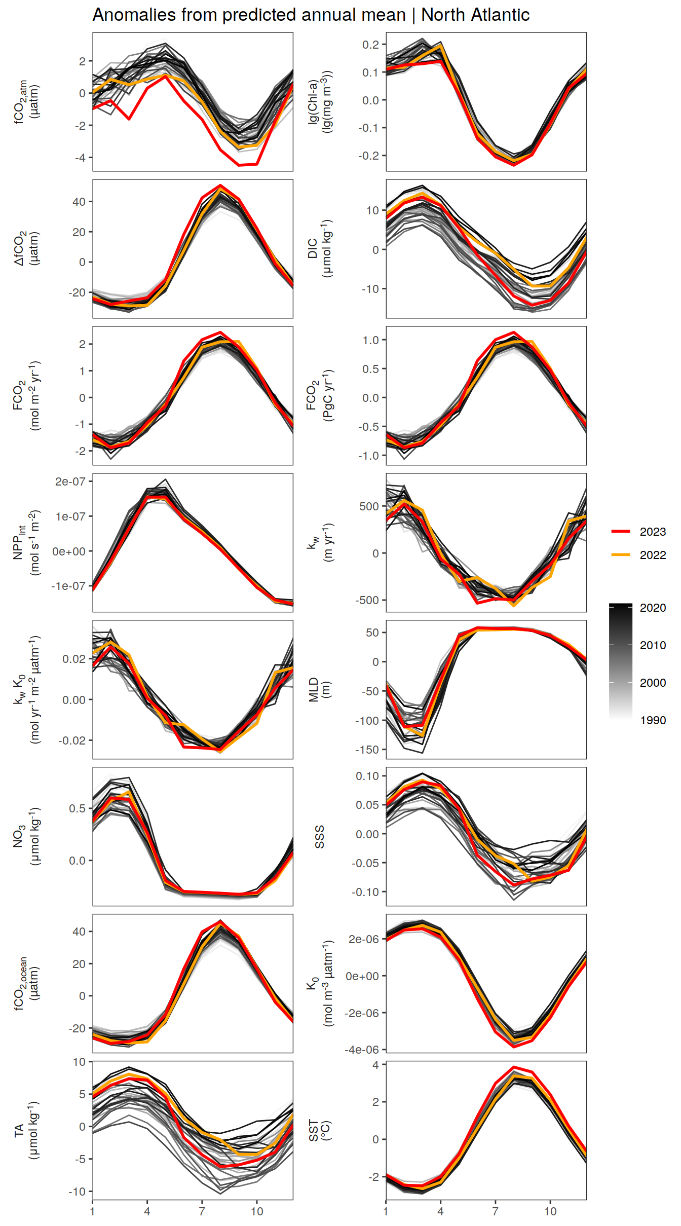
[[2]]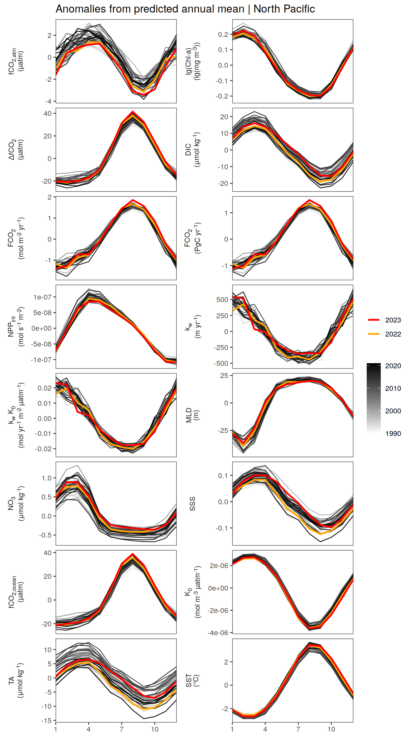
pco2_product_annual_detrended %>%
  write_csv(paste0("../data/","FESOM-REcoM","_","2023","_biome_annual_detrended.csv"))
Monthly mean trends
pco2_product_monthly %>%
  filter(biome %in% "Global") %>%
  mutate(month = as.factor(month)) %>%
  ggplot(aes(year, value, col = month)) +
  # geom_point() +
  geom_smooth(data = . %>% filter(year != 2023,
                                  !(name %in% name_quadratic_fit)),
              method = "lm",
              se = FALSE,
              fullrange = TRUE) +
  geom_smooth(
    data = . %>% filter(year != 2023,
                        name %in% name_quadratic_fit),
    method = "lm",
    fullrange = TRUE,
    formula = y ~ x + I(x ^ 2),
    se = FALSE
  ) +
  scale_color_scico_d(palette = "romaO",
    name = paste("Regression fit\nexcl.", 2023)) +
  scale_x_continuous(breaks = seq(1980, 2020, 20)) +
  labs(title = "Monthly mean trends | Global") +
  facet_wrap(name ~ .,
             scales = "free_y",
             labeller = labeller(name = x_axis_labels),
             strip.position = "left",
             ncol = 2) +
  theme(
    strip.text.y.left = element_markdown(),
    strip.placement = "outside",
    strip.background.y = element_blank(),
    axis.title = element_blank()
  )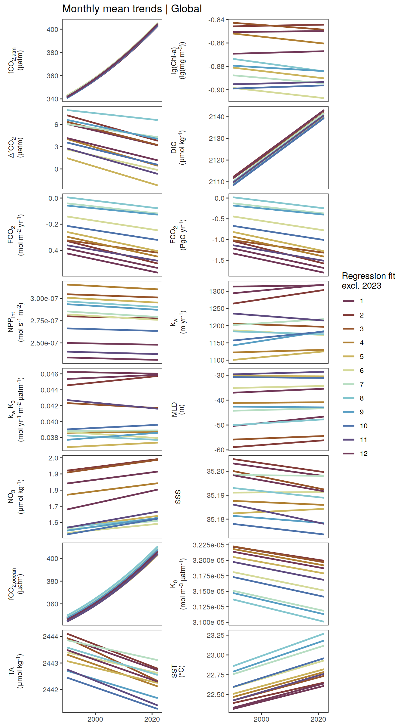
| Version | Author | Date |
|---|---|---|
| 054921b | jens-daniel-mueller | 2024-05-23 |
| 38f6f6e | jens-daniel-mueller | 2024-05-22 |
| be285dc | jens-daniel-mueller | 2024-05-21 |
| 51df30d | jens-daniel-mueller | 2024-05-15 |
| 009791f | jens-daniel-mueller | 2024-05-14 |
| 3b5d16b | jens-daniel-mueller | 2024-05-13 |
| fb21e78 | jens-daniel-mueller | 2024-05-08 |
| c7897dc | jens-daniel-mueller | 2024-05-08 |
pco2_product_monthly %>%
  filter(biome %in% key_biomes) %>%
  mutate(month = as.factor(month)) %>%
  ggplot(aes(year, value, col = month)) +
  # geom_point() +
  geom_smooth(data = . %>% filter(year != 2023,
                                  !(name %in% name_quadratic_fit)),
              method = "lm",
              fullrange = TRUE,
              se = FALSE) +
  geom_smooth(
    data = . %>% filter(year != 2023,
                        name %in% name_quadratic_fit),
    method = "lm",
    fullrange = TRUE,
    formula = y ~ x + I(x ^ 2),
    se = FALSE
  ) +
  scale_color_scico_d(palette = "romaO",
    name = paste("Regression fit\nexcl.", 2023)) +
  scale_x_continuous(breaks = seq(1980, 2020, 20)) +
  labs(title = "Monthly mean trends | Selected biomes") +
  facet_grid(name ~ biome,
             scales = "free_y",
             labeller = labeller(name = x_axis_labels),
             switch = "y") +
  theme(
    strip.text.y.left = element_markdown(),
    strip.placement = "outside",
    strip.background.y = element_blank(),
    axis.title = element_blank()
  )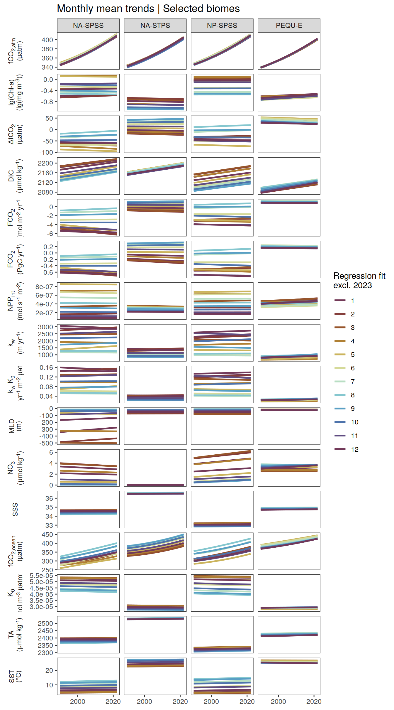
| Version | Author | Date |
|---|---|---|
| 054921b | jens-daniel-mueller | 2024-05-23 |
| 38f6f6e | jens-daniel-mueller | 2024-05-22 |
| be285dc | jens-daniel-mueller | 2024-05-21 |
| 51df30d | jens-daniel-mueller | 2024-05-15 |
| 009791f | jens-daniel-mueller | 2024-05-14 |
| 3b5d16b | jens-daniel-mueller | 2024-05-13 |
| fb21e78 | jens-daniel-mueller | 2024-05-08 |
| c7897dc | jens-daniel-mueller | 2024-05-08 |
pco2_product_monthly_regression <-
  pco2_product_monthly %>%
  anomaly_determination(biome, month)


pco2_product_monthly_regression %>%
  filter(biome %in% "Global") %>%
  group_split(month) %>%
  head(1) %>%
  map(
    ~ ggplot(data = .x,
             aes(year, resid)) +
      geom_hline(yintercept = 0) +
      geom_path() +
      geom_point(
        data = . %>% filter(!between(year, 2023-1, 2023)),
        aes(fill = year),
        shape = 21
      ) +
      scale_fill_grayC() +
      new_scale_fill() +
      geom_point(
        data = . %>% filter(between(year, 2023-1, 2023)),
        aes(fill = as.factor(year)),
        shape = 21,
        size = 2
      )  +
      scale_fill_manual(
        values = c("orange", "red"),
        guide = guide_legend(reverse = TRUE,
                             order = 1)
      ) +
      scale_x_continuous(breaks = seq(1980, 2020, 20)) +
      labs(title = "Residual from fit to monthly means (actual - predicted) | Global",
           subtitle = paste("Month:", .x$month)) +
      facet_wrap(
        name ~ .,
        scales = "free_y",
        labeller = labeller(name = x_axis_labels),
        strip.position = "left",
        ncol = 2
      ) +
      theme(
        strip.text.y.left = element_markdown(),
        strip.placement = "outside",
        strip.background.y = element_blank(),
        axis.title = element_blank(),
        legend.title = element_blank()
      )
  )
[[1]]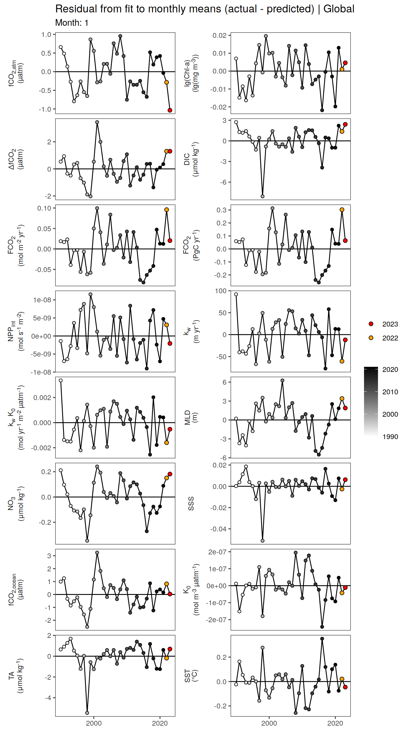
| Version | Author | Date |
|---|---|---|
| 054921b | jens-daniel-mueller | 2024-05-23 |
| 38f6f6e | jens-daniel-mueller | 2024-05-22 |
| be285dc | jens-daniel-mueller | 2024-05-21 |
| 51df30d | jens-daniel-mueller | 2024-05-15 |
| 009791f | jens-daniel-mueller | 2024-05-14 |
| 3b5d16b | jens-daniel-mueller | 2024-05-13 |
| fb21e78 | jens-daniel-mueller | 2024-05-08 |
| c7897dc | jens-daniel-mueller | 2024-05-08 |
pco2_product_monthly_regression %>%
  filter(biome %in% key_biomes) %>%
  group_split(month) %>%
  head(1) %>%
  map(
    ~ ggplot(data = .x,
             aes(year, resid)) +
      geom_hline(yintercept = 0) +
      geom_path() +
      geom_point(
        data = . %>% filter(!between(year, 2023-1, 2023)),
        aes(fill = year),
        shape = 21
      ) +
      scale_fill_grayC() +
      new_scale_fill() +
      geom_point(
        data = . %>% filter(between(year, 2023-1, 2023)),
        aes(fill = as.factor(year)),
        shape = 21,
        size = 2
      )  +
      scale_fill_manual(
        values = c("orange", "red"),
        guide = guide_legend(reverse = TRUE,
                             order = 1)
      ) +
      scale_x_continuous(breaks = seq(1980, 2020, 20)) +
      labs(title = "Residual from fit to monthly means (actual - predicted) | Selected biomes",
           subtitle = paste("Month:", .x$month)) +
      facet_grid(
        name ~ biome,
        scales = "free_y",
        labeller = labeller(name = x_axis_labels),
        switch = "y"
      ) +
      theme(
        strip.text.y.left = element_markdown(),
        strip.placement = "outside",
        strip.background.y = element_blank(),
        axis.title = element_blank(),
        legend.title = element_blank()
      )
  )
[[1]]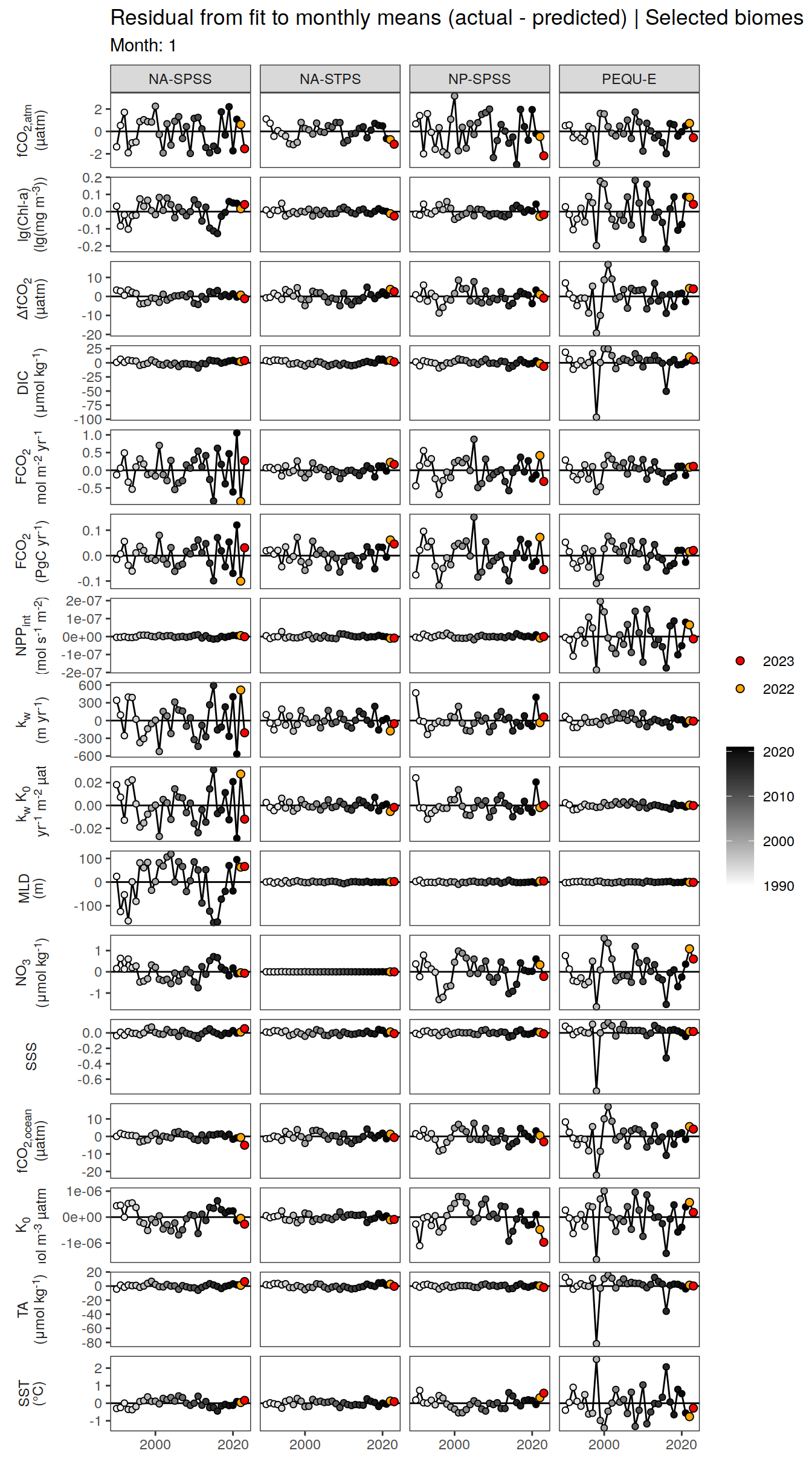
| Version | Author | Date |
|---|---|---|
| 054921b | jens-daniel-mueller | 2024-05-23 |
| 38f6f6e | jens-daniel-mueller | 2024-05-22 |
| be285dc | jens-daniel-mueller | 2024-05-21 |
| 51df30d | jens-daniel-mueller | 2024-05-15 |
| 009791f | jens-daniel-mueller | 2024-05-14 |
| 3b5d16b | jens-daniel-mueller | 2024-05-13 |
| fb21e78 | jens-daniel-mueller | 2024-05-08 |
| c7897dc | jens-daniel-mueller | 2024-05-08 |
pco2_product_monthly_regression %>%
  write_csv(paste0("../data/","FESOM-REcoM","_","2023","_biome_monthly_regression.csv"))
Global
pco2_product_monthly_detrended <-
  full_join(pco2_product_monthly,
            pco2_product_monthly_regression %>% select(-c(value, resid, time))) %>%
  mutate(resid = value - fit)

pco2_product_monthly_detrended %>%
  filter(biome %in% "Global") %>%
  ggplot(aes(month, resid, group = as.factor(year))) +
  geom_path(data = . %>% filter(!between(year, 2023-1, 2023)),
            aes(col = year)) +
  scale_color_grayC() +
  new_scale_color() +
  geom_path(data = . %>% filter(between(year, 2023-1, 2023)),
            aes(col = as.factor(year)),
            linewidth = 1) +
  scale_color_manual(values = c("orange", "red"),
                     guide = guide_legend(reverse = TRUE,
                                          order = 1)) +
  scale_x_continuous(breaks = seq(1, 12, 3), expand = c(0, 0)) +
  labs(title = "Anomalies from predicted monthly mean | Global") +
  facet_wrap(
    name ~ .,
    scales = "free_y",
    labeller = labeller(name = x_axis_labels),
    strip.position = "left",
    ncol = 2
  ) +
  theme(
    strip.text.y.left = element_markdown(),
    strip.placement = "outside",
    strip.background.y = element_blank(),
    axis.title.y = element_blank(),
    legend.title = element_blank()
  )
| Version | Author | Date |
|---|---|---|
| 054921b | jens-daniel-mueller | 2024-05-23 |
| 38f6f6e | jens-daniel-mueller | 2024-05-22 |
| be285dc | jens-daniel-mueller | 2024-05-21 |
| 51df30d | jens-daniel-mueller | 2024-05-15 |
| 009791f | jens-daniel-mueller | 2024-05-14 |
| 3b5d16b | jens-daniel-mueller | 2024-05-13 |
| fb21e78 | jens-daniel-mueller | 2024-05-08 |
| c7897dc | jens-daniel-mueller | 2024-05-08 |
pco2_product_monthly_detrended %>%
  filter(biome %in% key_biomes) %>%
  ggplot(aes(month, resid, group = as.factor(year))) +
  geom_path(data = . %>% filter(!between(year, 2023-1, 2023)),
            aes(col = year)) +
  scale_color_grayC() +
  new_scale_color() +
  geom_path(data = . %>% filter(between(year, 2023-1, 2023)),
            aes(col = as.factor(year)),
            linewidth = 1) +
  scale_color_manual(values = c("orange", "red"),
                     guide = guide_legend(reverse = TRUE,
                                          order = 1)) +
  scale_x_continuous(breaks = seq(1, 12, 3), expand = c(0, 0)) +
  labs(title = "Anomalies from predicted monthly mean | Selected biomes") +
  facet_grid(
    name ~ biome,
    scales = "free_y",
    labeller = labeller(name = x_axis_labels),
    switch = "y"
  ) +
  theme(
    strip.text.y.left = element_markdown(),
    strip.placement = "outside",
    strip.background.y = element_blank(),
    axis.title.y = element_blank(),
    legend.title = element_blank()
  )
| Version | Author | Date |
|---|---|---|
| 054921b | jens-daniel-mueller | 2024-05-23 |
| 38f6f6e | jens-daniel-mueller | 2024-05-22 |
| be285dc | jens-daniel-mueller | 2024-05-21 |
| 51df30d | jens-daniel-mueller | 2024-05-15 |
| 009791f | jens-daniel-mueller | 2024-05-14 |
| 3b5d16b | jens-daniel-mueller | 2024-05-13 |
| fb21e78 | jens-daniel-mueller | 2024-05-08 |
| c7897dc | jens-daniel-mueller | 2024-05-08 |
pco2_product_monthly_detrended %>%
  filter(biome %in% super_biomes) %>%
  ggplot(aes(month, resid, group = as.factor(year))) +
  geom_path(data = . %>% filter(!between(year, 2023-1, 2023)),
            aes(col = year)) +
  scale_color_grayC() +
  new_scale_color() +
  geom_path(data = . %>% filter(between(year, 2023-1, 2023)),
            aes(col = as.factor(year)),
            linewidth = 1) +
  scale_color_manual(values = c("orange", "red"),
                     guide = guide_legend(reverse = TRUE,
                                          order = 1)) +
  scale_x_continuous(breaks = seq(1, 12, 3), expand = c(0, 0)) +
  labs(title = "Anomalies from predicted monthly mean | Selected super biomes") +
  facet_grid(
    name ~ biome,
    scales = "free_y",
    labeller = labeller(name = x_axis_labels),
    switch = "y"
  ) +
  theme(
    strip.text.y.left = element_markdown(),
    strip.placement = "outside",
    strip.background.y = element_blank(),
    axis.title.y = element_blank(),
    legend.title = element_blank()
  )
| Version | Author | Date |
|---|---|---|
| 054921b | jens-daniel-mueller | 2024-05-23 |
| 38f6f6e | jens-daniel-mueller | 2024-05-22 |
| be285dc | jens-daniel-mueller | 2024-05-21 |
| 51df30d | jens-daniel-mueller | 2024-05-15 |
| 009791f | jens-daniel-mueller | 2024-05-14 |
| 3b5d16b | jens-daniel-mueller | 2024-05-13 |
| fb21e78 | jens-daniel-mueller | 2024-05-08 |
| c7897dc | jens-daniel-mueller | 2024-05-08 |
Selected biomes
pco2_product_monthly_detrended %>%
  filter(biome %in% key_biomes) %>%
  ggplot(aes(month, resid, group = as.factor(year))) +
  geom_path(data = . %>% filter(!between(year, 2023-1, 2023)),
            aes(col = year)) +
  scale_color_grayC() +
  new_scale_color() +
  geom_path(data = . %>% filter(between(year, 2023-1, 2023)),
            aes(col = as.factor(year)),
            linewidth = 1) +
  scale_color_manual(values = c("orange", "red"),
                     guide = guide_legend(reverse = TRUE,
                                          order = 1)) +
  scale_x_continuous(breaks = seq(1, 12, 3), expand = c(0, 0)) +
  labs(title = "Anomalies from predicted monthly mean | Selected biomes") +
  facet_grid(
    name ~ biome,
    scales = "free_y",
    labeller = labeller(name = x_axis_labels),
    switch = "y"
  ) +
  theme(
    strip.text.y.left = element_markdown(),
    strip.placement = "outside",
    strip.background.y = element_blank(),
    axis.title.y = element_blank(),
    legend.title = element_blank()
  )
| Version | Author | Date |
|---|---|---|
| 054921b | jens-daniel-mueller | 2024-05-23 |
| 38f6f6e | jens-daniel-mueller | 2024-05-22 |
| be285dc | jens-daniel-mueller | 2024-05-21 |
| 51df30d | jens-daniel-mueller | 2024-05-15 |
| 009791f | jens-daniel-mueller | 2024-05-14 |
| 3b5d16b | jens-daniel-mueller | 2024-05-13 |
| fb21e78 | jens-daniel-mueller | 2024-05-08 |
| c7897dc | jens-daniel-mueller | 2024-05-08 |
pco2_product_monthly_detrended %>%
  filter(biome %in% key_biomes) %>%
  group_split(biome) %>%
  # head(1) %>%
  map(
    ~ ggplot(data = .x,
             aes(month, resid, group = as.factor(year))) +
      geom_path(data = . %>% filter(!between(year, 2023-1, 2023)),
                aes(col = year)) +
      scale_color_grayC() +
      new_scale_color() +
      geom_path(
        data = . %>% filter(between(year, 2023-1, 2023)),
        aes(col = as.factor(year)),
        linewidth = 1
      ) +
      scale_color_manual(
        values = c("orange", "red"),
        guide = guide_legend(reverse = TRUE,
                             order = 1)
      ) +
      scale_x_continuous(breaks = seq(1, 12, 3), expand = c(0, 0)) +
      labs(title = paste("Anomalies from predicted monthly mean |", .x$biome)) +
      facet_wrap(
        name ~ .,
        scales = "free_y",
        labeller = labeller(name = x_axis_labels),
        strip.position = "left",
        ncol = 2
      ) +
      theme(
        strip.text.y.left = element_markdown(),
        strip.placement = "outside",
        strip.background.y = element_blank(),
        axis.title.y = element_blank(),
        legend.title = element_blank()
      )
  )
[[1]]
[[2]]
[[3]]
[[4]]
Super biomes
pco2_product_monthly_detrended %>%
  filter(biome %in% super_biomes) %>%
  ggplot(aes(month, resid, group = as.factor(year))) +
  geom_path(data = . %>% filter(!between(year, 2023-1, 2023)),
            aes(col = year)) +
  scale_color_grayC() +
  new_scale_color() +
  geom_path(data = . %>% filter(between(year, 2023-1, 2023)),
            aes(col = as.factor(year)),
            linewidth = 1) +
  scale_color_manual(values = c("orange", "red"),
                     guide = guide_legend(reverse = TRUE,
                                          order = 1)) +
  scale_x_continuous(breaks = seq(1, 12, 3), expand = c(0, 0)) +
  labs(title = "Anomalies from predicted monthly mean | Selected super biomes") +
  facet_grid(
    name ~ biome,
    scales = "free_y",
    labeller = labeller(name = x_axis_labels),
    switch = "y"
  ) +
  theme(
    strip.text.y.left = element_markdown(),
    strip.placement = "outside",
    strip.background.y = element_blank(),
    axis.title.y = element_blank(),
    legend.title = element_blank()
  )
| Version | Author | Date |
|---|---|---|
| 054921b | jens-daniel-mueller | 2024-05-23 |
| 38f6f6e | jens-daniel-mueller | 2024-05-22 |
| be285dc | jens-daniel-mueller | 2024-05-21 |
| 51df30d | jens-daniel-mueller | 2024-05-15 |
| 009791f | jens-daniel-mueller | 2024-05-14 |
| 3b5d16b | jens-daniel-mueller | 2024-05-13 |
| fb21e78 | jens-daniel-mueller | 2024-05-08 |
| c7897dc | jens-daniel-mueller | 2024-05-08 |
pco2_product_monthly_detrended %>%
  filter(biome %in% super_biomes) %>%
  group_split(biome) %>%
  # head(1) %>%
  map(
    ~ ggplot(data = .x,
             aes(month, resid, group = as.factor(year))) +
      geom_path(data = . %>% filter(!between(year, 2023-1, 2023)),
                aes(col = year)) +
      scale_color_grayC() +
      new_scale_color() +
      geom_path(
        data = . %>% filter(between(year, 2023-1, 2023)),
        aes(col = as.factor(year)),
        linewidth = 1
      ) +
      scale_color_manual(
        values = c("orange", "red"),
        guide = guide_legend(reverse = TRUE,
                             order = 1)
      ) +
      scale_x_continuous(breaks = seq(1, 12, 3), expand = c(0, 0)) +
      labs(title = paste("Anomalies from predicted monthly mean |", .x$biome)) +
      facet_wrap(
        name ~ .,
        scales = "free_y",
        labeller = labeller(name = x_axis_labels),
        strip.position = "left",
        ncol = 2
      ) +
      theme(
        strip.text.y.left = element_markdown(),
        strip.placement = "outside",
        strip.background.y = element_blank(),
        axis.title.y = element_blank(),
        legend.title = element_blank()
      )
  )
[[1]]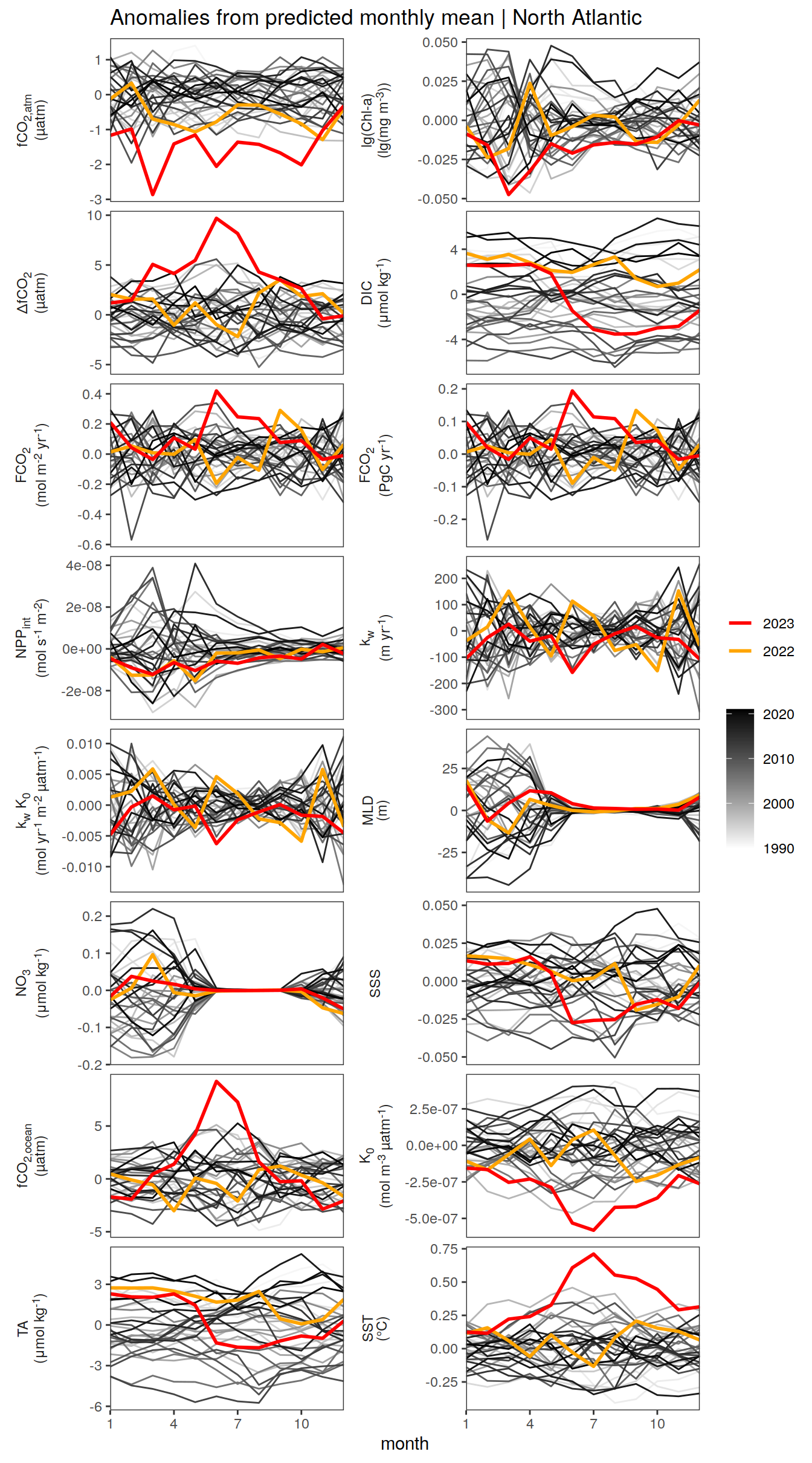
[[2]]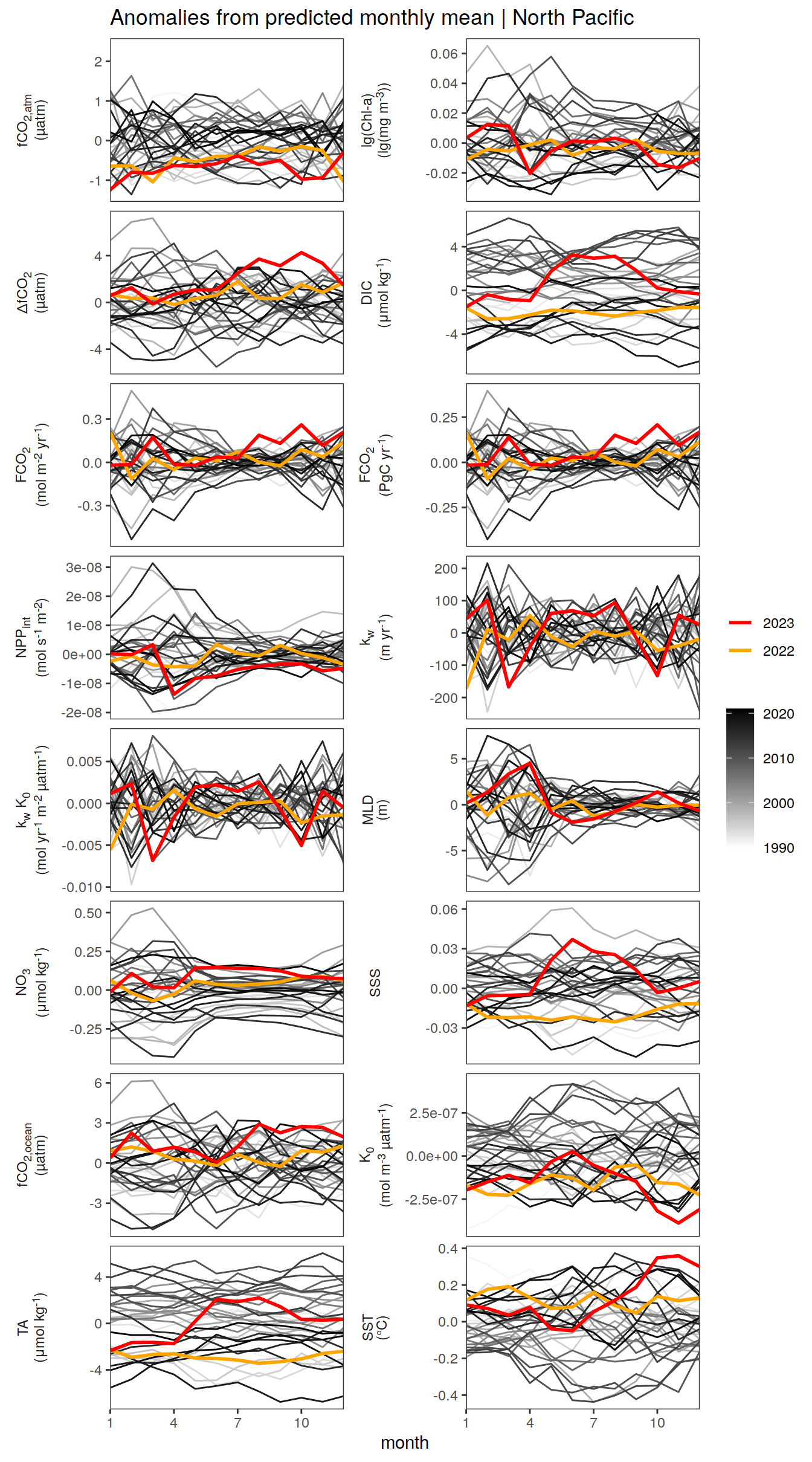
pco2_product_monthly_detrended %>%
  write_csv(paste0("../data/","FESOM-REcoM","_","2023","_biome_monthly_detrended.csv"))
2023 anomaly correlation
The following plots aim to unravel the correlation between regionally integrated monthly flux anomalies and the corresponding anomalies of the means/integrals of each other variable.
Anomalies are first presented are first presented in absolute units. Due to the different flux magnitudes, we need to plot integrated fluxes separately for each region. Secondly, we normalize the monthly anomalies to the spread (expressed as standard deviation) of the residuals from the fit.
Annual anomalies
Absolute
pco2_product_annual_regression %>%
  filter(biome == "Global") %>%
  select(-c(value, fit)) %>%
  pivot_wider(values_from = resid) %>%
  pivot_longer(-c(year, biome, fgco2_int))  %>%
  ggplot(aes(value, fgco2_int)) +
  geom_hline(yintercept = 0) +
  geom_point(data = . %>% filter(!between(year, 2023-1, 2023)),
             aes(fill = year),
             shape = 21) +
  geom_smooth(
    data = . %>% filter(!between(year, 2023-1, 2023)),
    method = "lm",
    se = FALSE,
    fullrange = TRUE,
    aes(col = paste("Regression fit\nexcl.", 2023))
  ) +
  scale_color_grey() +
  scale_fill_grayC()+
  new_scale_fill() +
  geom_point(data = . %>% filter(between(year, 2023-1, 2023)),
             aes(fill = as.factor(year)),
             shape = 21, size = 2)  +
  scale_fill_manual(values = c("orange", "red"),
                     guide = guide_legend(reverse = TRUE,
                                          order = 1)) +
  labs(title = "Globally integrated fluxes",
       y = labels_breaks("fgco2_int")$i_legend_title) +
  facet_wrap(
    ~ name,
    scales = "free_x",
    labeller = labeller(name = x_axis_labels),
    strip.position = "bottom",
    ncol = 2
  ) +
  theme(
    strip.text.x.bottom = element_markdown(),
    strip.placement = "outside",
    strip.background.x = element_blank(),
    axis.title.y = element_markdown(),
    axis.title.x = element_blank(),
    legend.title = element_blank()
  )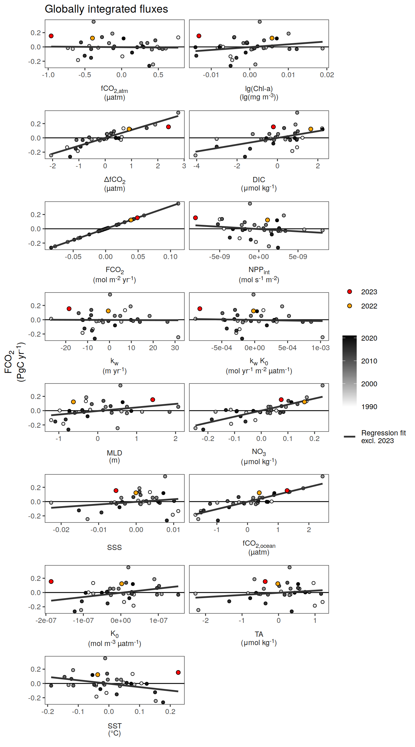
| Version | Author | Date |
|---|---|---|
| 054921b | jens-daniel-mueller | 2024-05-23 |
| 38f6f6e | jens-daniel-mueller | 2024-05-22 |
| be285dc | jens-daniel-mueller | 2024-05-21 |
| 51df30d | jens-daniel-mueller | 2024-05-15 |
| 009791f | jens-daniel-mueller | 2024-05-14 |
| 3b5d16b | jens-daniel-mueller | 2024-05-13 |
| fb21e78 | jens-daniel-mueller | 2024-05-08 |
| c7897dc | jens-daniel-mueller | 2024-05-08 |
Monthly anomalies
Absolute
pco2_product_monthly_detrended_anomaly <-
  pco2_product_monthly_detrended %>%
  select(year, month, biome, name, resid) %>%
  pivot_wider(names_from = name,
              values_from = resid)


pco2_product_monthly_detrended_anomaly %>%
  filter(biome == "Global") %>%
  pivot_longer(-c(year, month, biome, fgco2_int))  %>%
  ggplot(aes(value, fgco2_int)) +
  geom_hline(yintercept = 0) +
  geom_point(data = . %>% filter(year != 2023),
             aes(col = paste(min(year), max(year), sep = "-")),
             alpha = 0.2) +
  geom_smooth(
    data = . %>% filter(year != 2023),
    aes(col = paste(min(year), max(year), sep = "-")),
    method = "lm",
    se = FALSE,
    fullrange = TRUE
  )  +
  scale_color_grey(name = "") +
  new_scale_color() +
  geom_path(data = . %>% filter(year == 2023),
            aes(col = as.factor(month), group = 1))  +
  geom_point(data = . %>% filter(year == 2023),
             aes(fill =  as.factor(month)),
             shape = 21,
             size = 3)  +
  scale_color_scico_d(palette = "buda",
                     guide = guide_legend(reverse = TRUE,
                                          order = 1),
                     name = paste("Month\nof", 2023)) +
  scale_fill_scico_d(palette = "buda",
                     guide = guide_legend(reverse = TRUE,
                                          order = 1),
                     name = paste("Month\nof", 2023)) +
  labs(title = "Globally integrated fluxes",
       y = labels_breaks("fgco2_int")$i_legend_title) +
  facet_wrap(
    ~ name,
    scales = "free_x",
    labeller = labeller(name = x_axis_labels),
    strip.position = "bottom",
    ncol = 2
  ) +
  theme(
    strip.text.x.bottom = element_markdown(),
    strip.placement = "outside",
    strip.background.x = element_blank(),
    axis.title.y = element_markdown(),
    axis.title.x = element_blank()
  )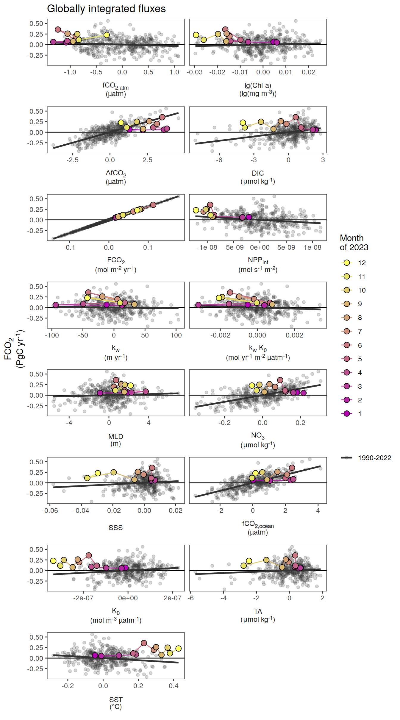
| Version | Author | Date |
|---|---|---|
| 054921b | jens-daniel-mueller | 2024-05-23 |
| 38f6f6e | jens-daniel-mueller | 2024-05-22 |
| be285dc | jens-daniel-mueller | 2024-05-21 |
| 51df30d | jens-daniel-mueller | 2024-05-15 |
| 009791f | jens-daniel-mueller | 2024-05-14 |
| 3b5d16b | jens-daniel-mueller | 2024-05-13 |
| fb21e78 | jens-daniel-mueller | 2024-05-08 |
| c7897dc | jens-daniel-mueller | 2024-05-08 |
pco2_product_monthly_detrended_anomaly %>%
  filter(!(biome %in% c(super_biomes, "Global"))) %>%
  pivot_longer(-c(year, month, biome, fgco2_int))  %>%
  group_split(name) %>%
  # head(1) %>%
  map(
    ~ ggplot(data = .x,
             aes(value, fgco2_int)) +
      geom_hline(yintercept = 0) +
      geom_point(
        data = . %>% filter(year != 2023),
        aes(col = paste(min(year), max(year), sep = "-")),
        alpha = 0.2
      ) +
      geom_smooth(
        data = . %>% filter(year != 2023),
        aes(col = paste(min(year), max(year), sep = "-")),
        method = "lm",
        se = FALSE,
        fullrange = TRUE
      )  +
      scale_color_grey(name = "") +
      new_scale_color() +
      geom_path(data = . %>% filter(year == 2023),
                aes(col = as.factor(month), group = 1))  +
      geom_point(
        data = . %>% filter(year == 2023),
        aes(fill = as.factor(month)),
        shape = 21,
        size = 3
      )  +
      scale_color_scico_d(
        palette = "buda",
        guide = guide_legend(reverse = TRUE,
                             order = 1),
        name = paste("Month\nof", 2023)
      ) +
      scale_fill_scico_d(
        palette = "buda",
        guide = guide_legend(reverse = TRUE,
                             order = 1),
        name = paste("Month\nof", 2023)
      ) +
      facet_wrap( ~ biome, ncol = 3, scales = "free") +
      labs(
        title = "Biome integrated fluxes",
        y = labels_breaks("fgco2_int")$i_legend_title,
        x = labels_breaks(.x %>% distinct(name))$i_legend_title
      ) +
      theme(axis.title.x = element_markdown(),
            axis.title.y = element_markdown())
  )
[[1]]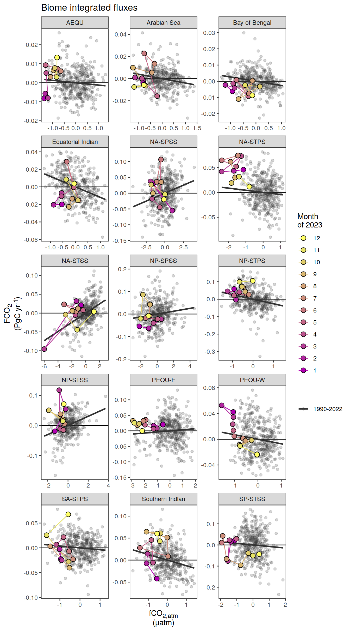
[[2]]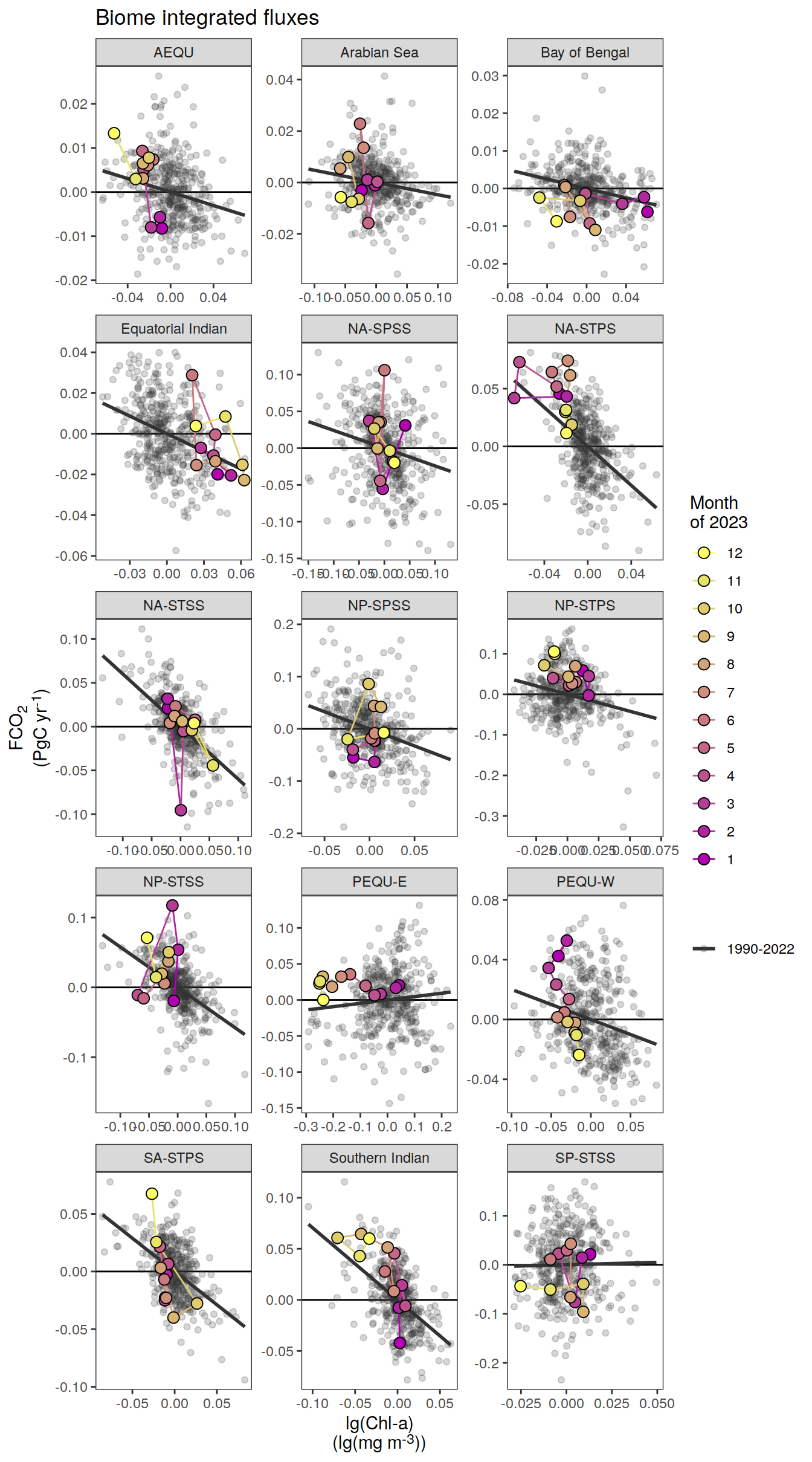
[[3]]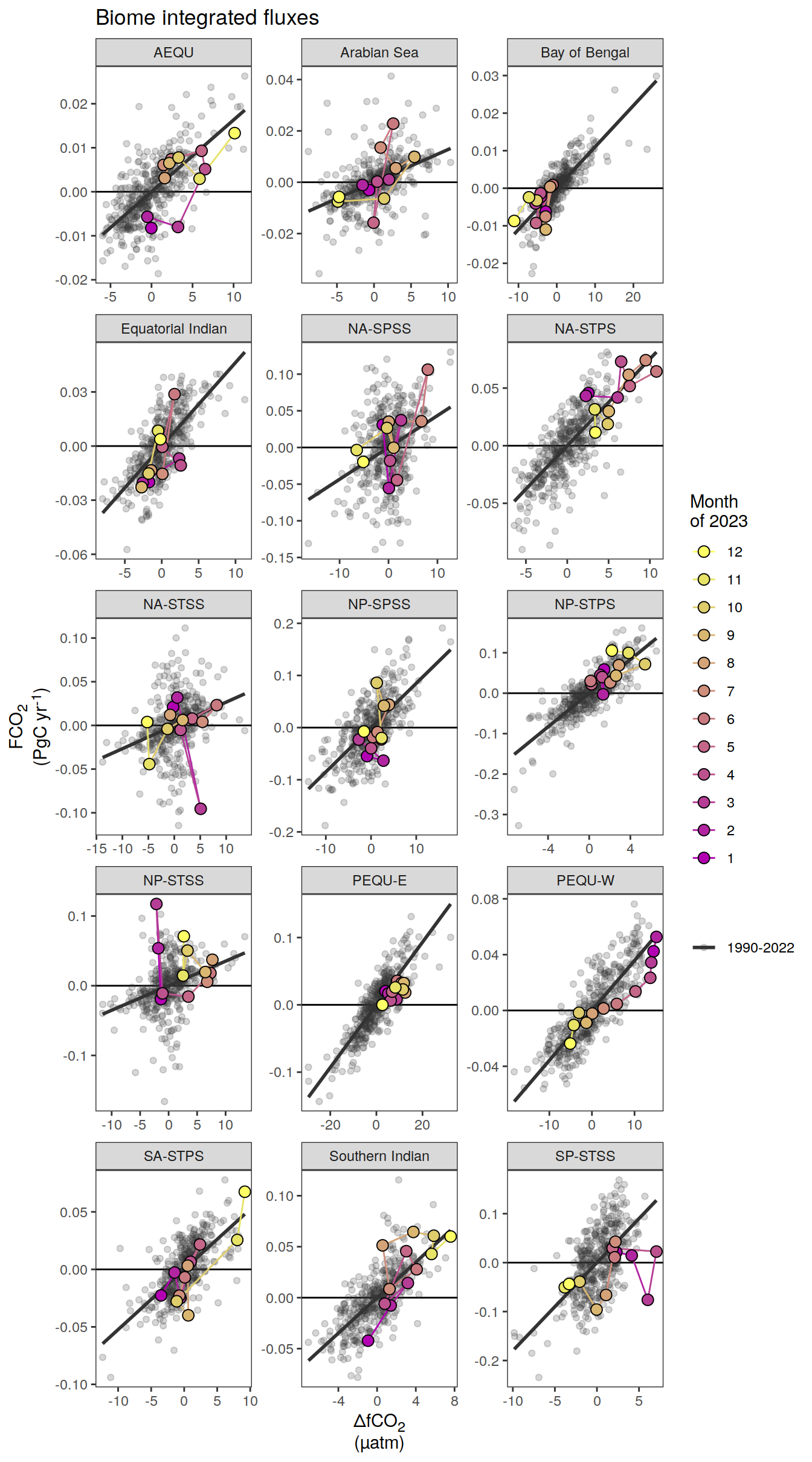
[[4]]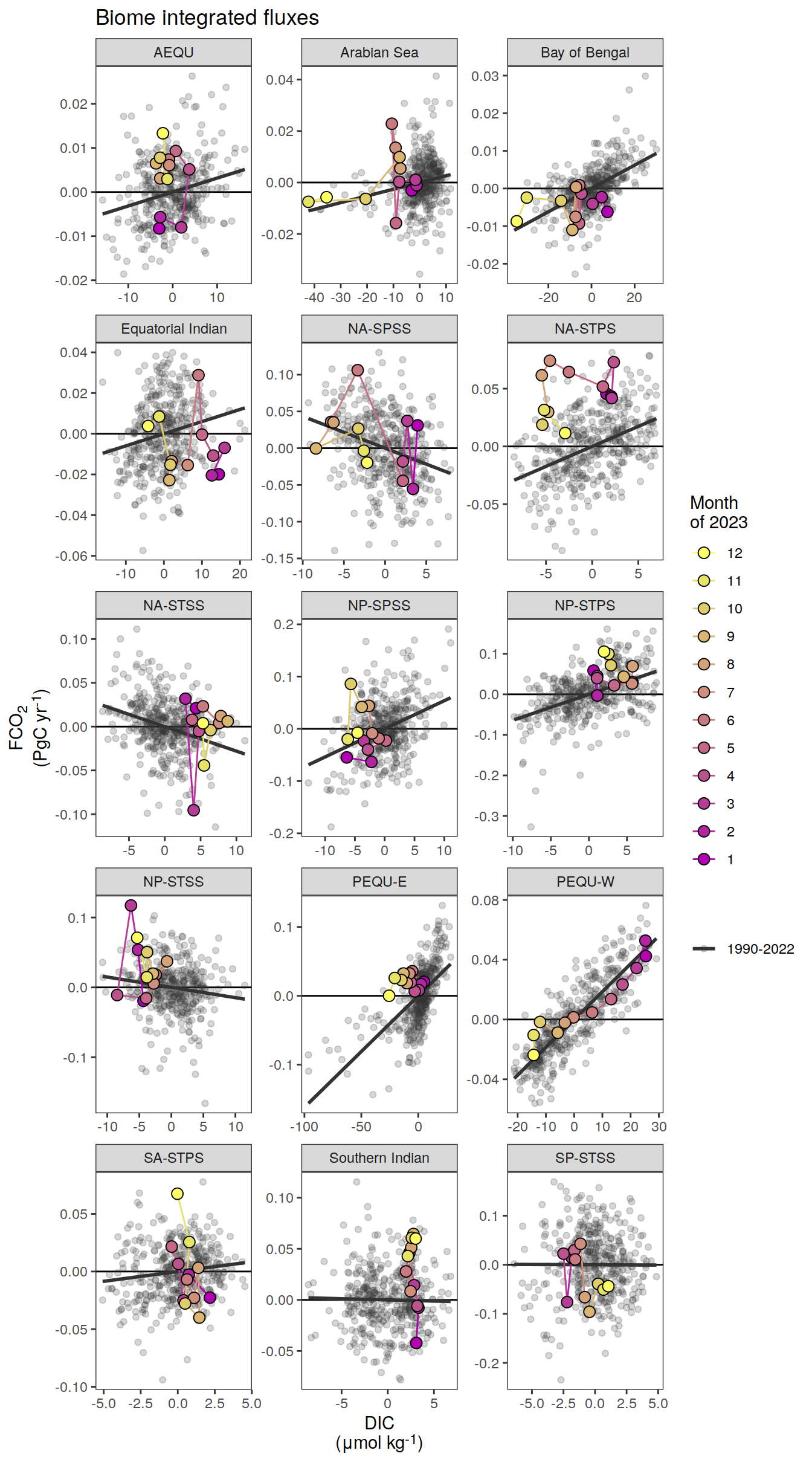
[[5]]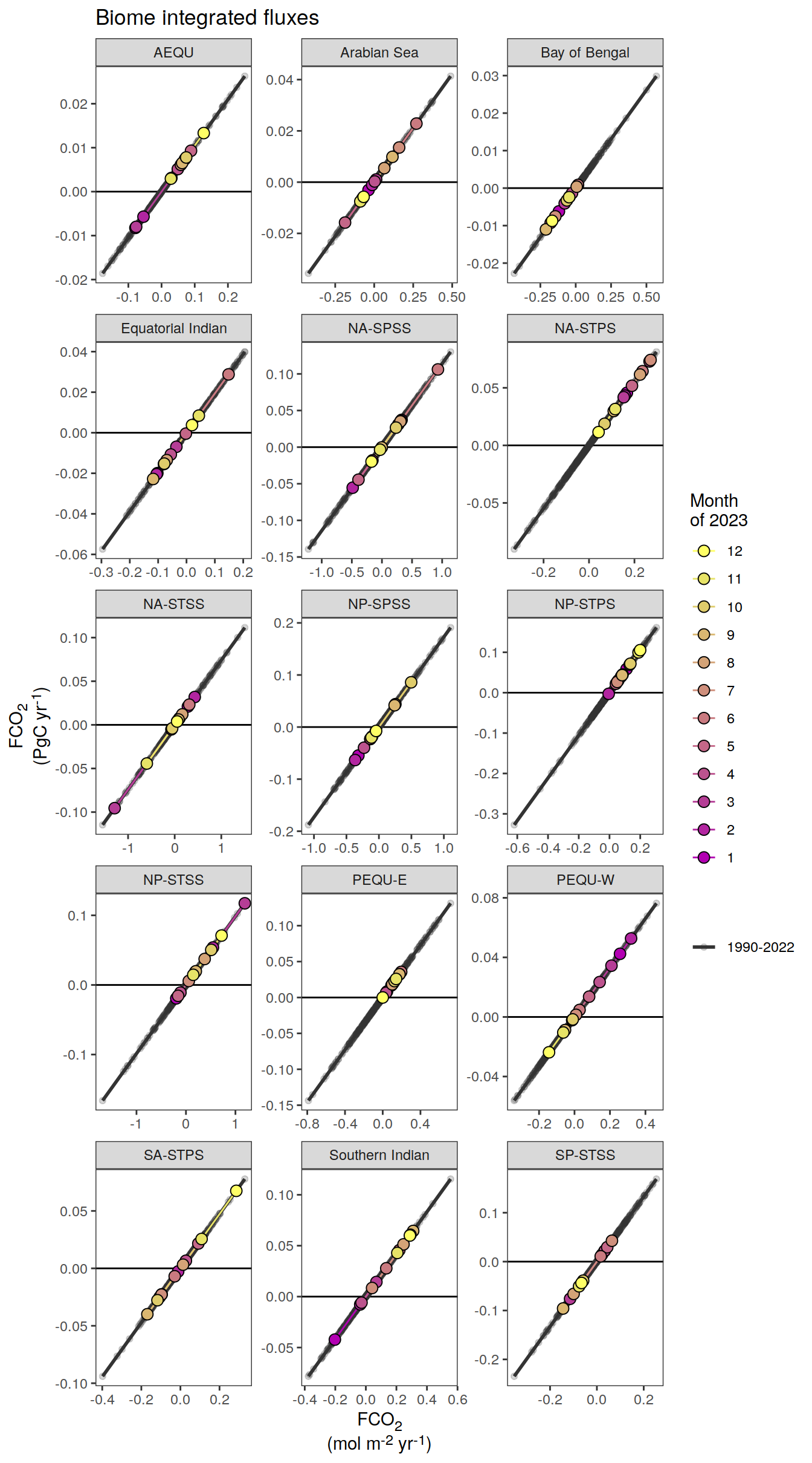
[[6]]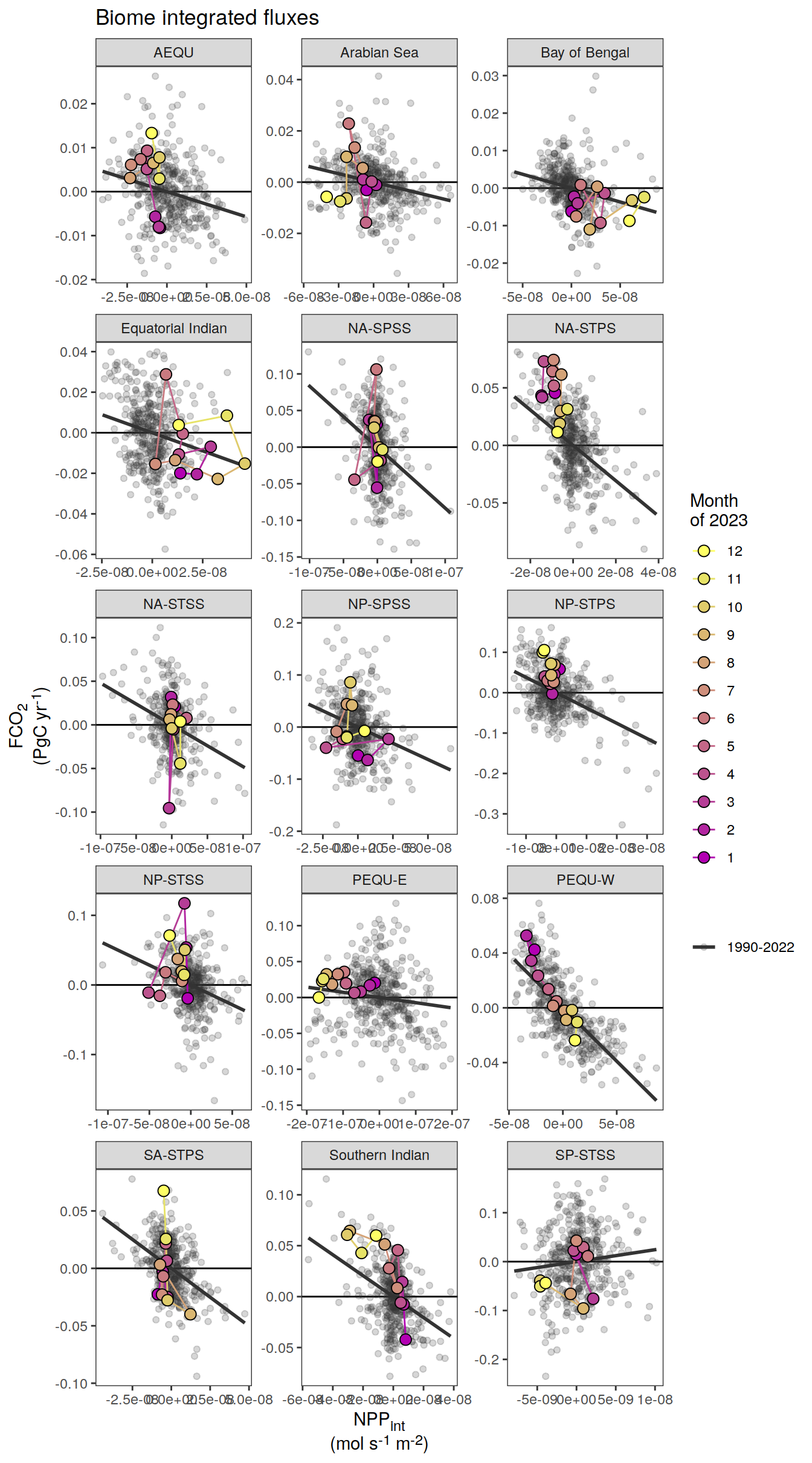
[[7]]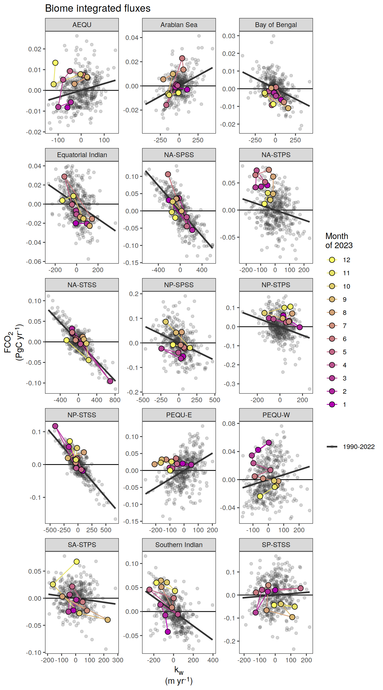
[[8]]
[[9]]
[[10]]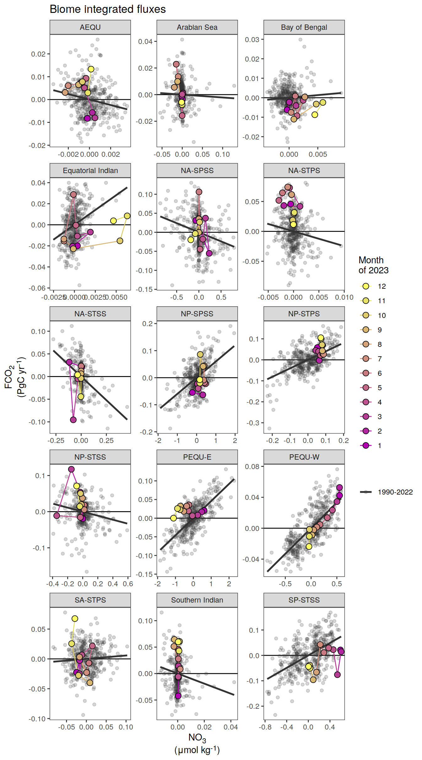
[[11]]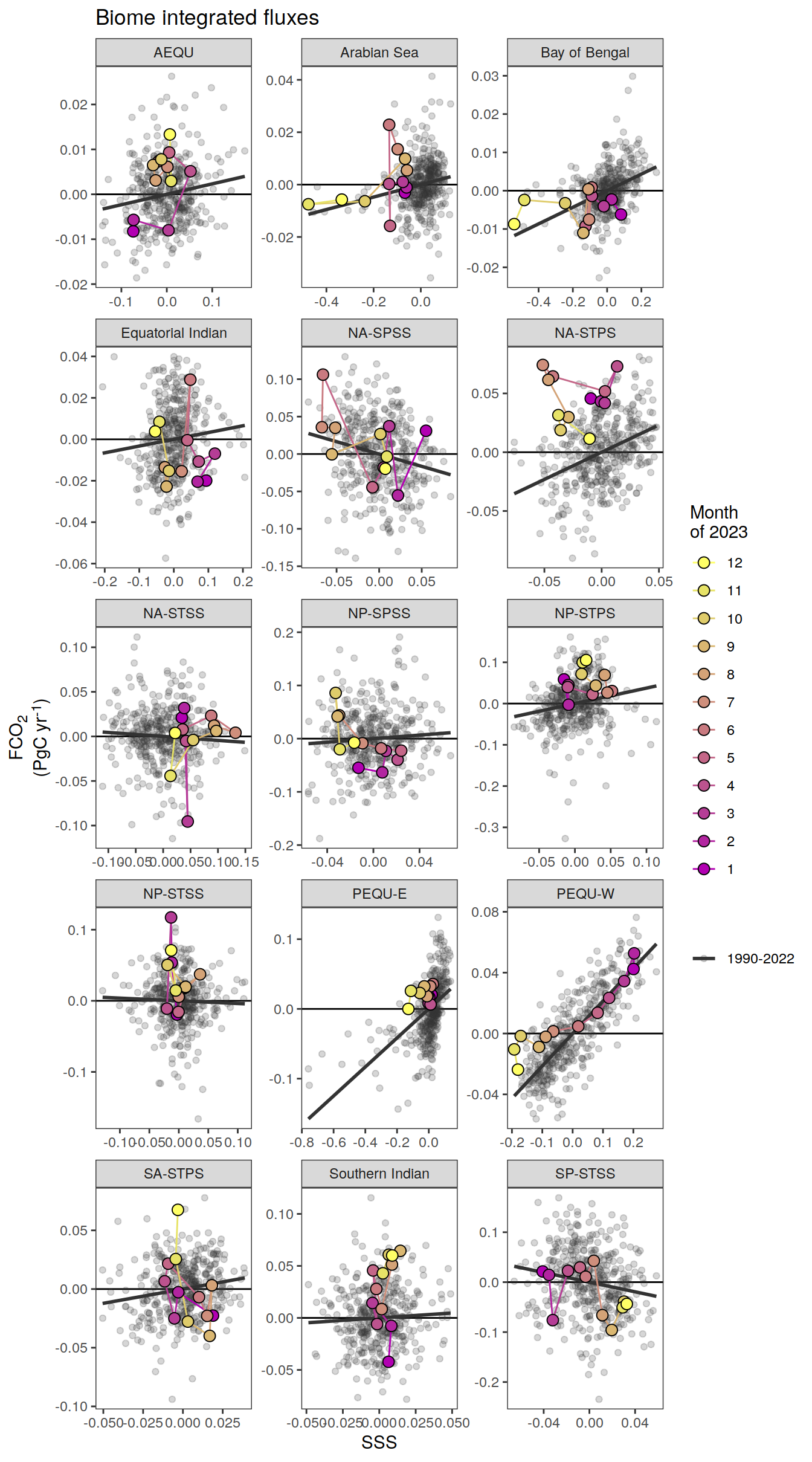
[[12]]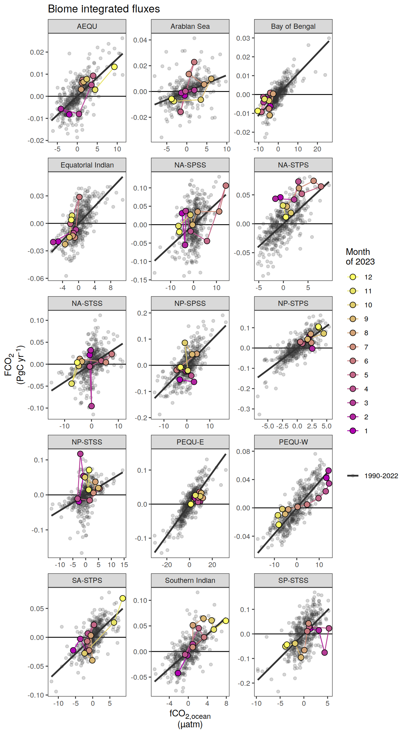
[[13]]
| Version | Author | Date |
|---|---|---|
| 054921b | jens-daniel-mueller | 2024-05-23 |
[[14]]
| Version | Author | Date |
|---|---|---|
| 054921b | jens-daniel-mueller | 2024-05-23 |
[[15]]
pco2_product_monthly_detrended_anomaly %>%
  filter(biome %in% super_biomes) %>%
  pivot_longer(-c(year, month, biome, fgco2_int))  %>%
  group_split(name) %>%
  # head(1) %>%
  map(
    ~ ggplot(data = .x,
             aes(value, fgco2_int)) +
      geom_hline(yintercept = 0) +
      geom_point(
        data = . %>% filter(year != 2023),
        aes(col = paste(min(year), max(year), sep = "-")),
        alpha = 0.2
      ) +
      geom_smooth(
        data = . %>% filter(year != 2023),
        aes(col = paste(min(year), max(year), sep = "-")),
        method = "lm",
        se = FALSE,
        fullrange = TRUE
      )  +
      scale_color_grey(name = "") +
      new_scale_color() +
      geom_path(data = . %>% filter(year == 2023),
                aes(col = as.factor(month), group = 1))  +
      geom_point(
        data = . %>% filter(year == 2023),
        aes(fill = as.factor(month)),
        shape = 21,
        size = 3
      )  +
      scale_color_scico_d(
        palette = "buda",
        guide = guide_legend(reverse = TRUE,
                             order = 1),
        name = paste("Month\nof", 2023)
      ) +
      scale_fill_scico_d(
        palette = "buda",
        guide = guide_legend(reverse = TRUE,
                             order = 1),
        name = paste("Month\nof", 2023)
      ) +
      facet_wrap( ~ biome, ncol = 3, scales = "free_x") +
      labs(
        title = "Super biome integrated fluxes",
        y = labels_breaks("fgco2_int")$i_legend_title,
        x = labels_breaks(.x %>% distinct(name))$i_legend_title
      ) +
      theme(axis.title.x = element_markdown(),
            axis.title.y = element_markdown())
  )
[[1]]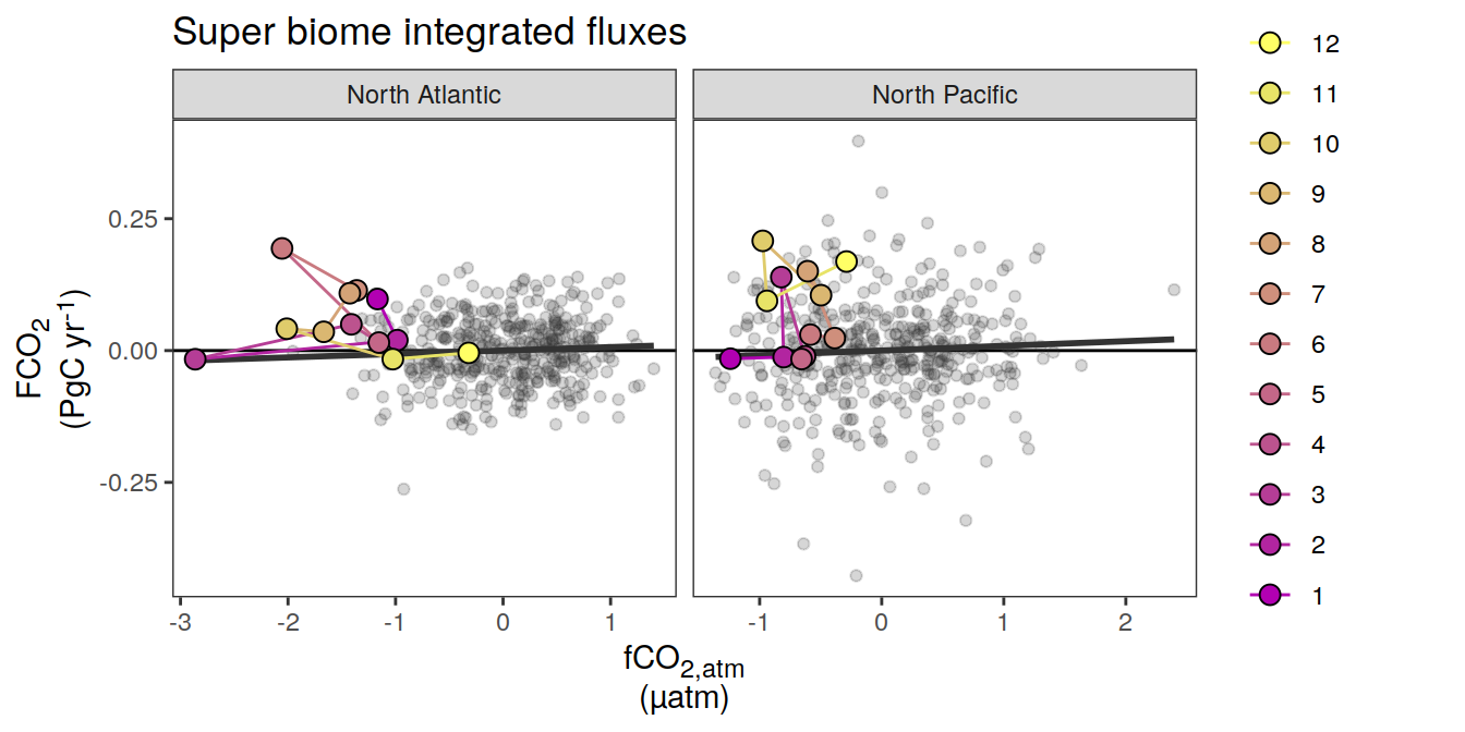
[[2]]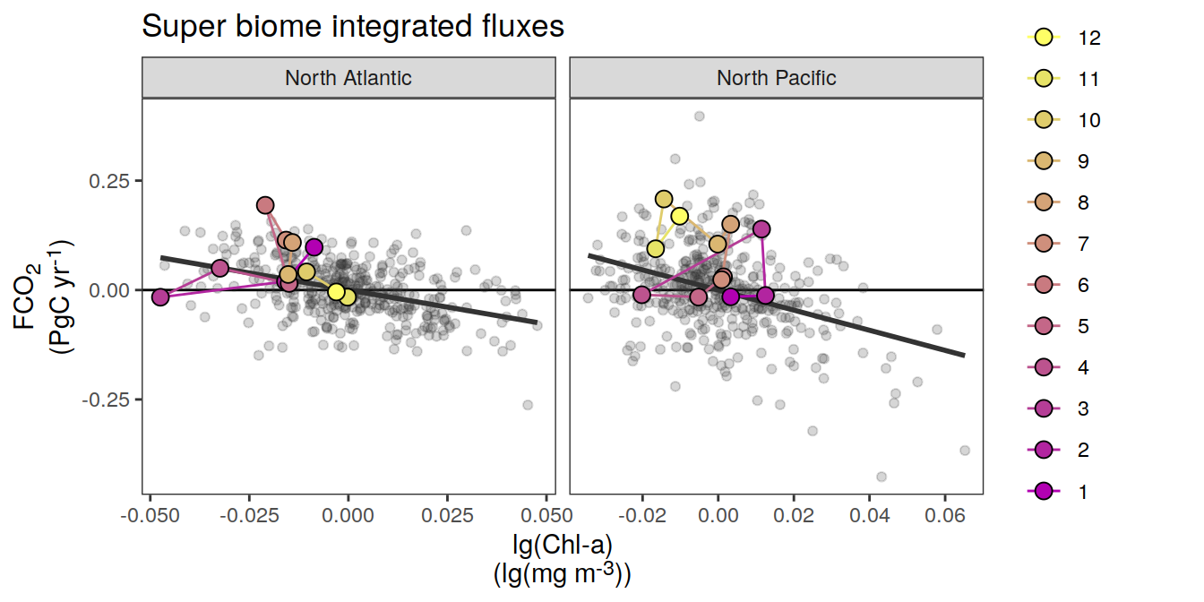
[[3]]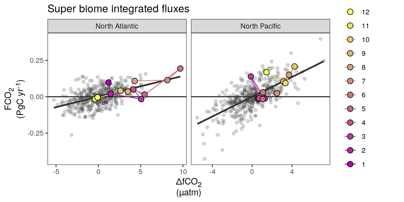
[[4]]
[[5]]
[[6]]
[[7]]
[[8]]
[[9]]
[[10]]
[[11]]
[[12]]
[[13]]
| Version | Author | Date |
|---|---|---|
| 054921b | jens-daniel-mueller | 2024-05-23 |
[[14]]
| Version | Author | Date |
|---|---|---|
| 054921b | jens-daniel-mueller | 2024-05-23 |
[[15]]
Relative to spread
pco2_product_monthly_detrended_anomaly_spread <-
  pco2_product_monthly_detrended_anomaly %>%
  pivot_longer(-c(month, biome, year)) %>%
  filter(year != 2023) %>%
  group_by(month, biome, name) %>%
  summarise(spread = sd(value, na.rm = TRUE)) %>%
  ungroup()


pco2_product_monthly_detrended_anomaly_relative <-
  full_join(
    pco2_product_monthly_detrended_anomaly_spread,
    pco2_product_monthly_detrended_anomaly %>%
      pivot_longer(-c(month, biome, year))
  )

pco2_product_monthly_detrended_anomaly_relative <-
  pco2_product_monthly_detrended_anomaly_relative %>%
  mutate(value = value / spread) %>%
  select(-spread) %>%
  pivot_wider() %>%
  pivot_longer(-c(month, biome, year, fgco2_int))


pco2_product_monthly_detrended_anomaly_relative %>%
  group_split(name) %>%
  # head(1) %>%
  map(
    ~ ggplot(data = .x,
             aes(value, fgco2_int)) +
      geom_vline(xintercept = 0) +
      geom_hline(yintercept = 0) +
      geom_point(
        data = . %>% filter(year != 2023),
        aes(col = paste(min(year), max(year), sep = "-")),
        alpha = 0.2
      ) +
      geom_smooth(
        data = . %>% filter(year != 2023),
        aes(col = paste(min(year), max(year), sep = "-")),
        method = "lm",
        se = FALSE,
        fullrange = TRUE
      )  +
      scale_color_grey(name = "") +
      new_scale_color() +
      geom_path(data = . %>% filter(year == 2023),
                aes(col = as.factor(month), group = 1))  +
      geom_point(
        data = . %>% filter(year == 2023),
        aes(fill = as.factor(month)),
        shape = 21,
        size = 3
      )  +
      scale_color_scico_d(
        palette = "buda",
        guide = guide_legend(reverse = TRUE,
                             order = 1),
        name = paste("Month\nof", 2023)
      ) +
      scale_fill_scico_d(
        palette = "buda",
        guide = guide_legend(reverse = TRUE,
                             order = 1),
        name = paste("Month\nof", 2023)
      ) +
      facet_wrap( ~ biome, ncol = 3) +
      coord_fixed() +
      labs(
        title = "Biome integrated fluxes normalized to spread",
        y = str_split_i(labels_breaks("fgco2_int")$i_legend_title, "<br>", i = 1),
        x = str_split_i(labels_breaks(.x %>% distinct(name))$i_legend_title, "<br>", i = 1)
      ) +
      theme(axis.title.x = element_markdown(),
            axis.title.y = element_markdown())
  )
[[1]]
[[2]]
[[3]]
[[4]]
[[5]]
[[6]]
[[7]]
[[8]]
[[9]]
[[10]]
[[11]]
[[12]]
[[13]]
| Version | Author | Date |
|---|---|---|
| 054921b | jens-daniel-mueller | 2024-05-23 |
[[14]]
| Version | Author | Date |
|---|---|---|
| 054921b | jens-daniel-mueller | 2024-05-23 |
[[15]]
Zonal mean sections
The following analysis is available for GOBMs only.
Annual means
2023 anomaly
pco2_product_zonal_mean_annual <-   pco2_product_zonal_mean %>%
  pivot_longer(-c(region, depth, lat, time, year, month)) %>%
  group_by(region, lat, depth, year, name) %>%
  summarise(value = mean(value)) %>%
  ungroup() %>%
  drop_na() %>%
  mutate(region = str_to_title(region))

pco2_product_zonal_mean_annual_regression <-
  pco2_product_zonal_mean_annual %>%
  anomaly_determination(region, lat, depth)

pco2_product_zonal_mean_annual_regression %>%
  filter(year == 2023) %>%
  group_split(name) %>%
  # head(3) %>%
  map(
    ~ ggplot(data = .x) +
      geom_contour_filled(aes(lat, depth, z = resid)) +
      scale_fill_discrete_divergingx(name = labels_breaks(.x %>% distinct(name))$i_legend_title) +
      guides(fill = guide_colorsteps(
        barheight = unit(8, "cm"),
        show.limits = TRUE
      )) +
      scale_y_continuous(trans = trans_reverser("sqrt"),
                         breaks = c(50,100,200,400)) +
      scale_x_continuous(breaks = seq(-100, 100, 20)) +
      coord_cartesian(expand = 0) +
      facet_wrap( ~ region, ncol = 1) +
      labs(y = "Depth (m)") +
      theme(legend.title = element_markdown())
  )
[[1]]
[[2]]
[[3]]
[[4]]
pco2_product_zonal_mean_annual_regression %>%
  write_csv(paste0("../data/","FESOM-REcoM","_","2023","_zonal_mean_sections_annual.csv"))
Biome profiles
The following analysis is available for GOBMs only.
Annual means
2023 anomaly
pco2_product_profiles_annual <-   pco2_product_profiles %>%
  pivot_longer(-c(biome, depth, time, year, month)) %>%
  group_by(biome, depth, year, name) %>%
  summarise(value = mean(value)) %>%
  ungroup() %>%
  drop_na()

pco2_product_profiles_annual_regression <-
  pco2_product_profiles_annual %>%
  anomaly_determination(biome, depth)

pco2_product_profiles_annual_regression %>%
  group_split(name) %>%
  # head(1) %>%
  map(
    ~ ggplot(data = .x) +
      geom_path(aes(resid, depth, group = year), col = "grey30", alpha = 0.5) +
      geom_path(data = .x %>% filter(year == 2023),
                aes(resid, depth, col = as.factor(year)),
                linewidth = 1) +
      scale_y_continuous(trans = trans_reverser("sqrt"),
                         breaks = c(50,100,200,400)) +
      facet_wrap( ~ biome) +
      labs(y = "Depth (m)",
           x = labels_breaks(.x %>% distinct(name))$i_legend_title) +
      theme(legend.title = element_blank(),
            axis.title.x = element_markdown())
  )
[[1]]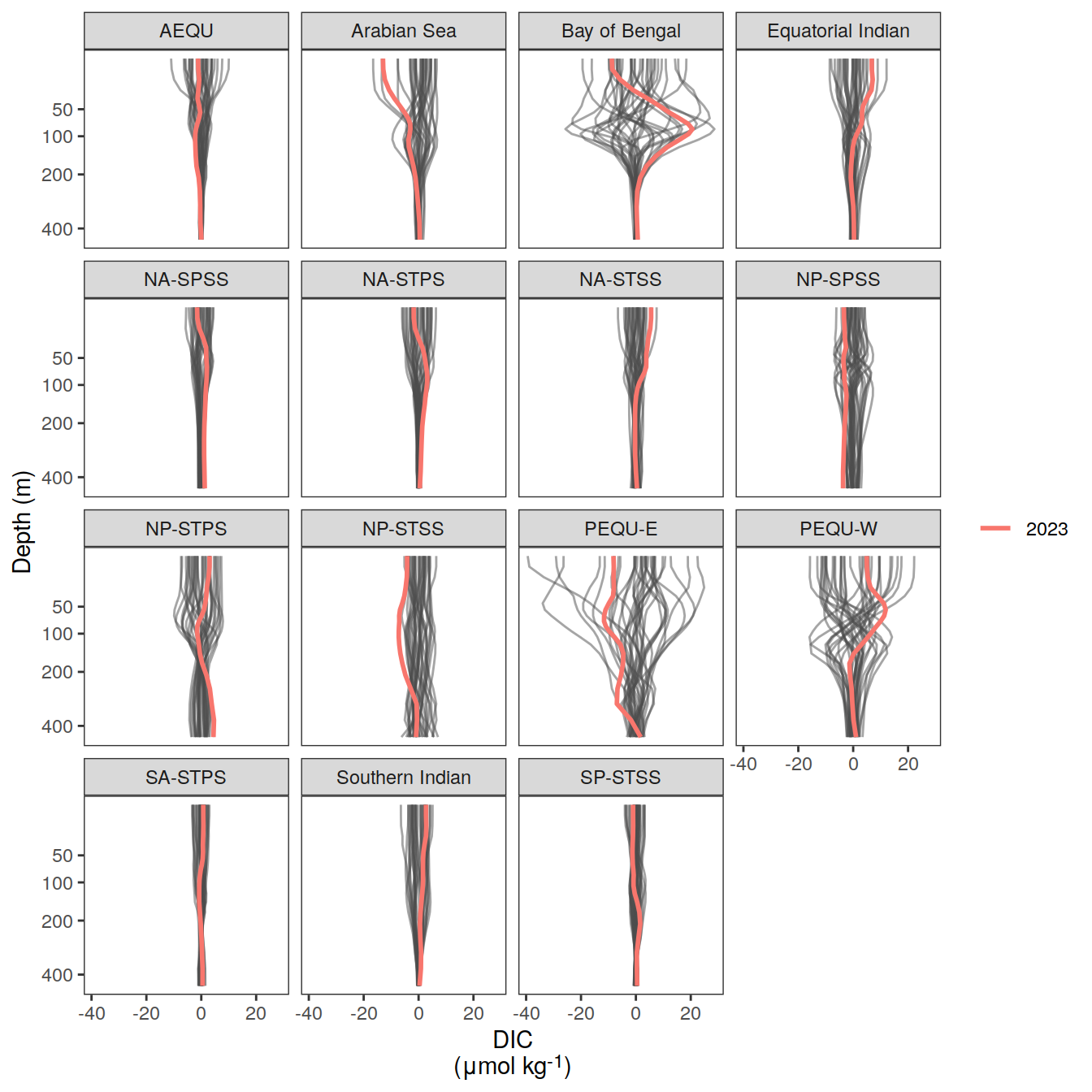
[[2]]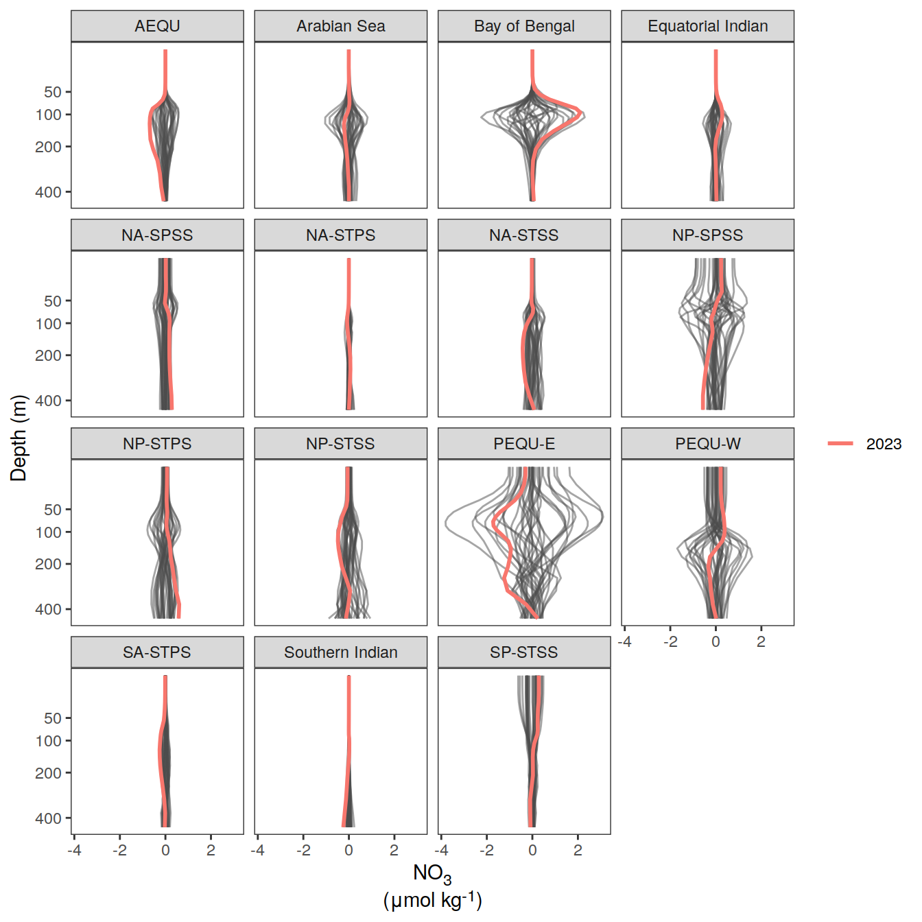
[[3]]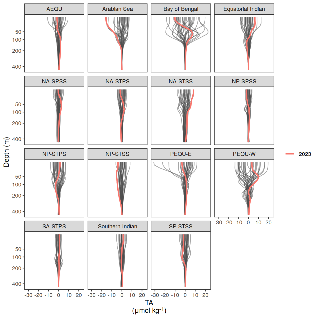
[[4]]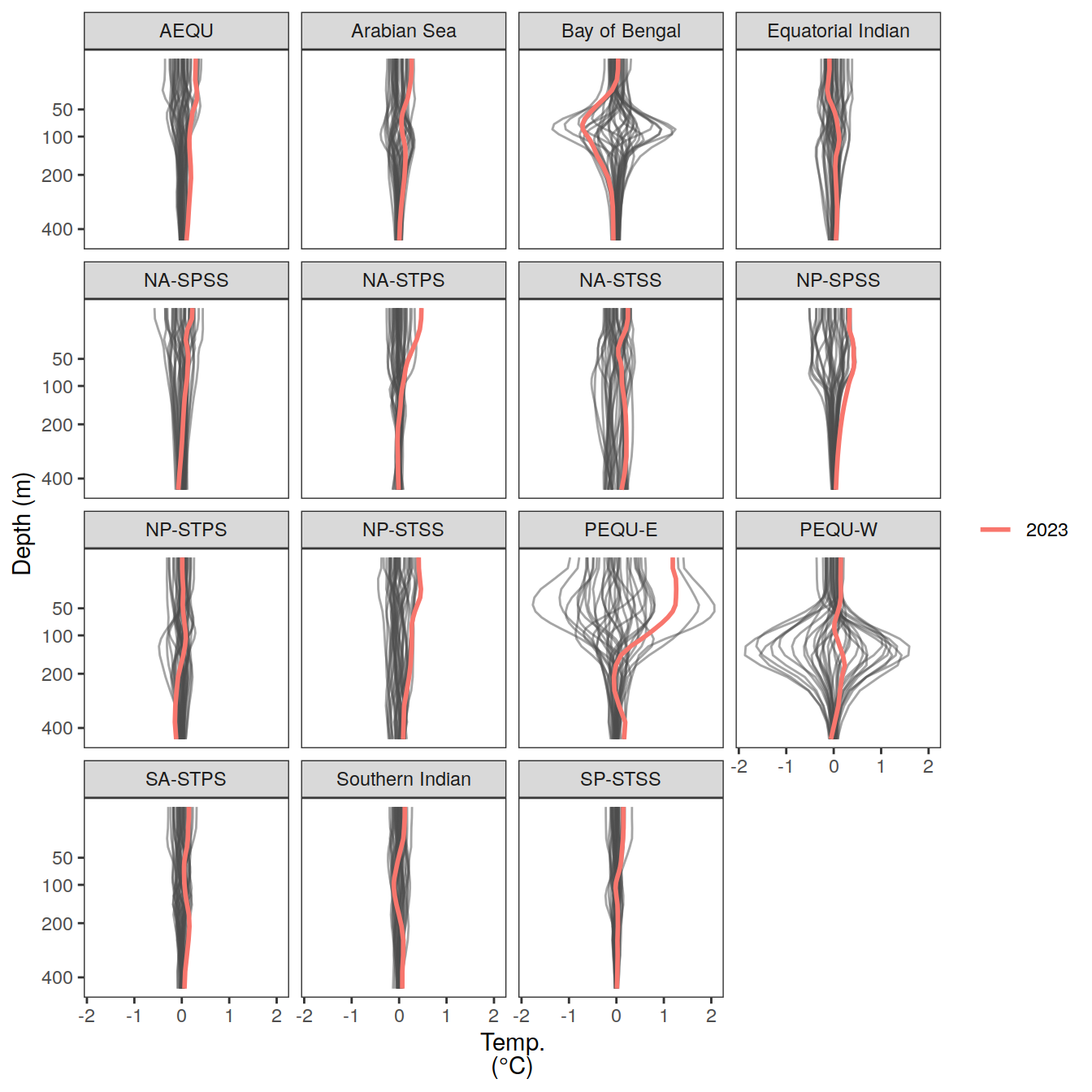
pco2_product_profiles_annual_regression %>%
  write_csv(paste0("../data/","FESOM-REcoM","_","2023","_profiles_annual.csv"))
Monthly means
2023 anomaly
pco2_product_profiles_monthly <-   pco2_product_profiles %>%
  pivot_longer(-c(biome, depth, time, year, month)) %>%
  group_by(biome, depth, year, month, name) %>%
  summarise(value = mean(value)) %>%
  ungroup() %>%
  drop_na()

pco2_product_profiles_monthly_regression <-
  pco2_product_profiles_monthly %>%
  anomaly_determination(biome, depth, month)

pco2_product_profiles_monthly_regression %>%
  filter(year == 2023) %>%
  group_split(name) %>%
  # head(1) %>%
  map(
    ~ ggplot(data = .x) +
      geom_vline(xintercept = 0) +
      geom_path(aes(resid, depth, col = as.factor(month)),
                linewidth = 1) +
      scale_color_scico_d(palette = "hawaii") +
      scale_y_continuous(trans = trans_reverser("sqrt"),
                         breaks = c(50, 100, 200, 400)) +
      facet_wrap(~ biome,
                 scales = "free_x") +
      labs(y = "Depth (m)",
           x = labels_breaks(.x %>% distinct(name))$i_legend_title) +
      theme(legend.title = element_blank(),
            axis.title.x = element_markdown())
  )
[[1]]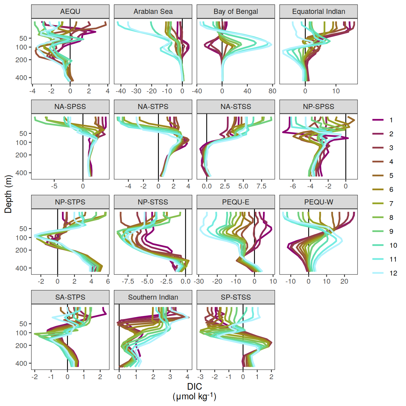
[[2]]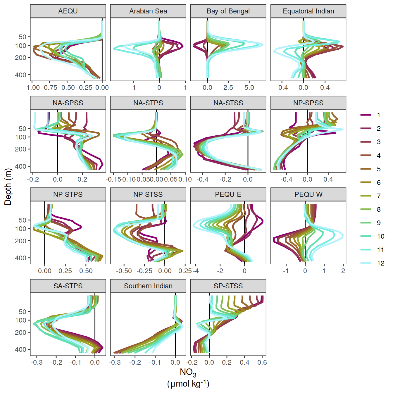
[[3]]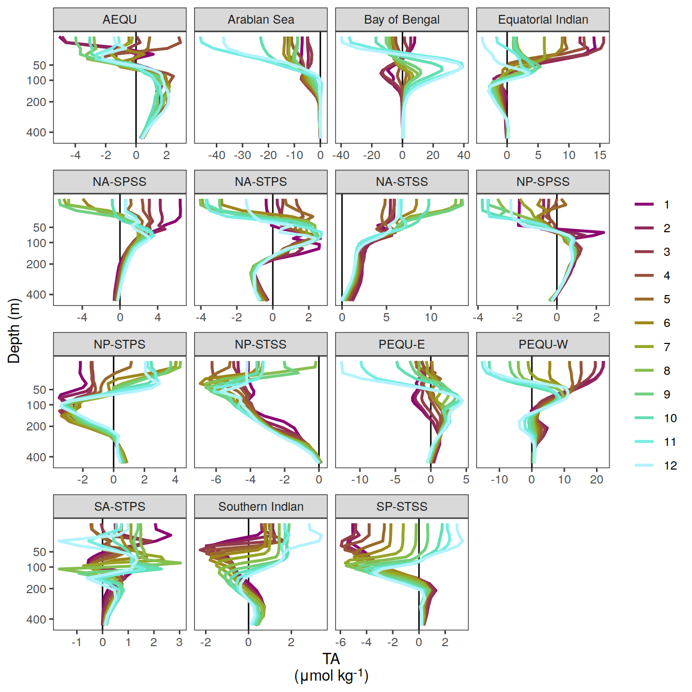
[[4]]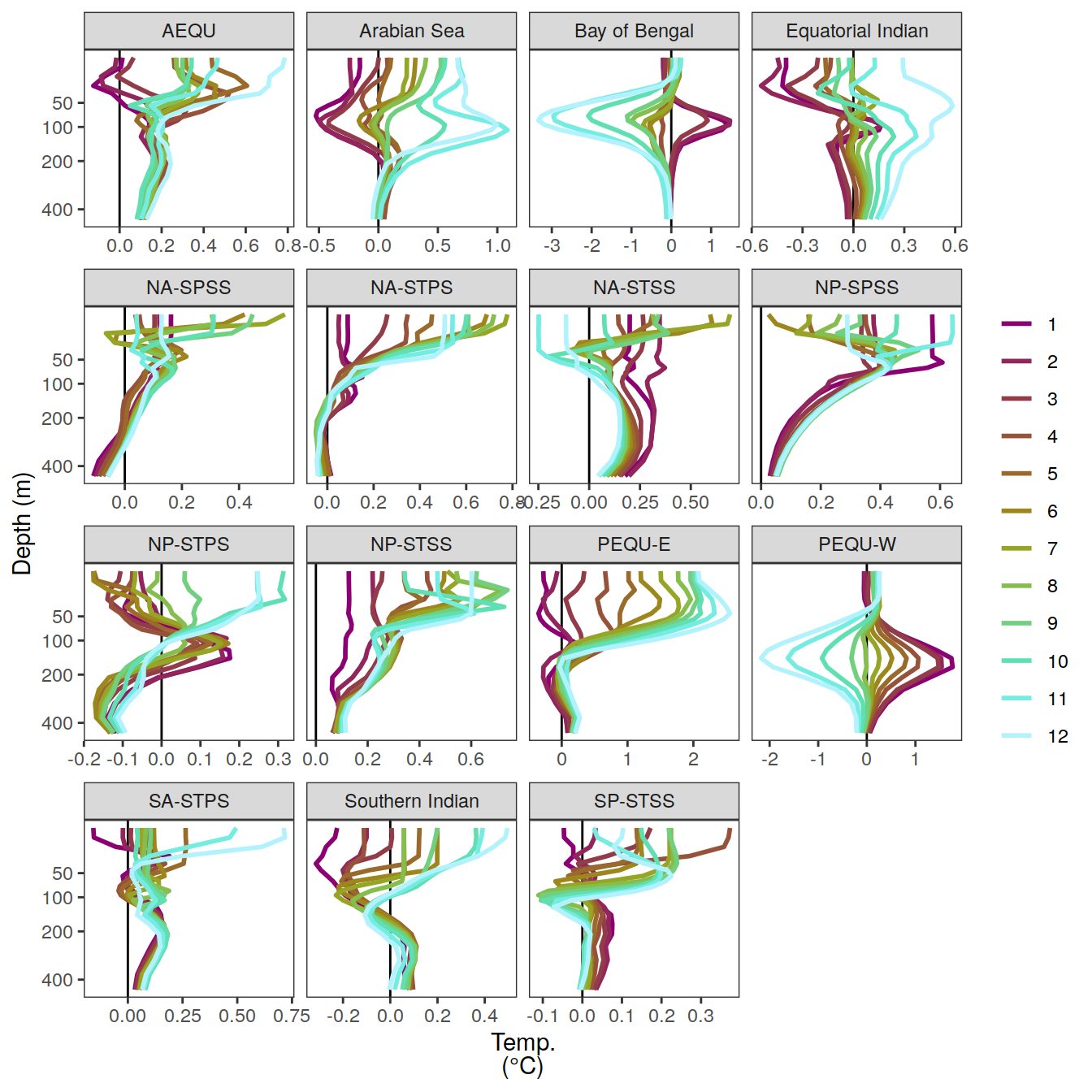
pco2_product_profiles_monthly_regression %>%
  write_csv(paste0("../data/","FESOM-REcoM","_","2023","_profiles_monthly.csv"))
sessionInfo()R version 4.2.2 (2022-10-31)
Platform: x86_64-pc-linux-gnu (64-bit)
Running under: openSUSE Leap 15.5
Matrix products: default
BLAS: /usr/local/R-4.2.2/lib64/R/lib/libRblas.so
LAPACK: /usr/local/R-4.2.2/lib64/R/lib/libRlapack.so
locale:
[1] LC_CTYPE=en_US.UTF-8 LC_NUMERIC=C
[3] LC_TIME=en_US.UTF-8 LC_COLLATE=en_US.UTF-8
[5] LC_MONETARY=en_US.UTF-8 LC_MESSAGES=en_US.UTF-8
[7] LC_PAPER=en_US.UTF-8 LC_NAME=C
[9] LC_ADDRESS=C LC_TELEPHONE=C
[11] LC_MEASUREMENT=en_US.UTF-8 LC_IDENTIFICATION=C
attached base packages:
[1] stats graphics grDevices utils datasets methods base
other attached packages:
[1] ggtext_0.1.2 broom_1.0.5 khroma_1.9.0
[4] ggnewscale_0.4.8 seacarb_3.3.1 SolveSAPHE_2.1.0
[7] oce_1.7-10 gsw_1.1-1 lubridate_1.9.0
[10] timechange_0.1.1 stars_0.6-0 abind_1.4-5
[13] terra_1.7-65 sf_1.0-9 rnaturalearth_0.1.0
[16] geomtextpath_0.1.1 colorspace_2.0-3 marelac_2.1.10
[19] shape_1.4.6 ggforce_0.4.1 metR_0.13.0
[22] scico_1.3.1 patchwork_1.1.2 collapse_1.8.9
[25] forcats_0.5.2 stringr_1.5.0 dplyr_1.1.3
[28] purrr_1.0.2 readr_2.1.3 tidyr_1.3.0
[31] tibble_3.2.1 ggplot2_3.4.4 tidyverse_1.3.2
[34] workflowr_1.7.0
loaded via a namespace (and not attached):
[1] readxl_1.4.1 backports_1.4.1 systemfonts_1.0.4
[4] lwgeom_0.2-10 sp_1.5-1 splines_4.2.2
[7] digest_0.6.30 htmltools_0.5.3 ncmeta_0.3.5
[10] fansi_1.0.3 magrittr_2.0.3 checkmate_2.1.0
[13] memoise_2.0.1 googlesheets4_1.0.1 tzdb_0.3.0
[16] modelr_0.1.10 vroom_1.6.0 rvest_1.0.3
[19] textshaping_0.3.6 haven_2.5.1 xfun_0.35
[22] callr_3.7.3 crayon_1.5.2 jsonlite_1.8.3
[25] glue_1.6.2 polyclip_1.10-4 gtable_0.3.1
[28] gargle_1.2.1 cubelyr_1.0.2 scales_1.2.1
[31] DBI_1.1.3 Rcpp_1.0.11 isoband_0.2.6
[34] viridisLite_0.4.1 gridtext_0.1.5 units_0.8-0
[37] bit_4.0.5 proxy_0.4-27 httr_1.4.4
[40] RColorBrewer_1.1-3 ellipsis_0.3.2 pkgconfig_2.0.3
[43] farver_2.1.1 sass_0.4.4 dbplyr_2.2.1
[46] utf8_1.2.2 here_1.0.1 tidyselect_1.2.0
[49] labeling_0.4.2 rlang_1.1.1 later_1.3.0
[52] munsell_0.5.0 cellranger_1.1.0 tools_4.2.2
[55] cachem_1.0.6 cli_3.6.1 generics_0.1.3
[58] evaluate_0.18 fastmap_1.1.0 yaml_2.3.6
[61] processx_3.8.0 knitr_1.41 bit64_4.0.5
[64] fs_1.5.2 RNetCDF_2.6-1 nlme_3.1-160
[67] whisker_0.4 xml2_1.3.3 compiler_4.2.2
[70] rstudioapi_0.15.0 e1071_1.7-12 reprex_2.0.2
[73] tweenr_2.0.2 bslib_0.4.1 stringi_1.7.8
[76] highr_0.9 ps_1.7.2 lattice_0.20-45
[79] Matrix_1.5-3 classInt_0.4-8 commonmark_1.8.1
[82] markdown_1.4 vctrs_0.6.4 pillar_1.9.0
[85] lifecycle_1.0.3 jquerylib_0.1.4 data.table_1.14.6
[88] httpuv_1.6.6 R6_2.5.1 promises_1.2.0.1
[91] KernSmooth_2.23-20 codetools_0.2-18 MASS_7.3-58.1
[94] assertthat_0.2.1 rprojroot_2.0.3 withr_2.5.0
[97] mgcv_1.8-41 parallel_4.2.2 hms_1.1.2
[100] grid_4.2.2 rnaturalearthdata_0.1.0 class_7.3-20
[103] rmarkdown_2.18 googledrive_2.0.0 git2r_0.30.1
[106] getPass_0.2-2