temperature_indices

workflowr

• Summary
• Checks
• Past versions

Last updated: 2024-11-05

Checks: 7 0

Knit directory: oae_ccs_roms/

This reproducible R Markdown analysis was created with workflowr (version 1.7.0). The Checks tab describes the reproducibility checks that were applied when the results were created. The Past versions tab lists the development history.

---

R Markdown file: up-to-date

Great! Since the R Markdown file has been committed to the Git repository, you know the exact version of the code that produced these results.

Environment: empty

Great job! The global environment was empty. Objects defined in the global environment can affect the analysis in your R Markdown file in unknown ways. For reproduciblity it’s best to always run the code in an empty environment.

Seed: set.seed(20240919)

The command set.seed(20240919) was run prior to running the code in the R Markdown file. Setting a seed ensures that any results that rely on randomness, e.g. subsampling or permutations, are reproducible.

Session information: recorded

Great job! Recording the operating system, R version, and package versions is critical for reproducibility.

Cache: none

Nice! There were no cached chunks for this analysis, so you can be confident that you successfully produced the results during this run.

File paths: relative

Great job! Using relative paths to the files within your workflowr project makes it easier to run your code on other machines.

Repository version: 0b73066

Great! You are using Git for version control. Tracking code development and connecting the code version to the results is critical for reproducibility.

The results in this page were generated with repository version 0b73066. See the Past versions tab to see a history of the changes made to the R Markdown and HTML files.

Note that you need to be careful to ensure that all relevant files for the analysis have been committed to Git prior to generating the results (you can use wflow_publish or wflow_git_commit). workflowr only checks the R Markdown file, but you know if there are other scripts or data files that it depends on. Below is the status of the Git repository when the results were generated:

Ignored files:
    Ignored:    .Rhistory
    Ignored:    .Rproj.user/

Unstaged changes:
    Modified:   analysis/_site.yml
    Modified:   code/Workflowr_project_managment.R

Note that any generated files, e.g. HTML, png, CSS, etc., are not included in this status report because it is ok for generated content to have uncommitted changes.

---

These are the previous versions of the repository in which changes were made to the R Markdown (analysis/temperature_indices.Rmd) and HTML (docs/temperature_indices.html) files. If you’ve configured a remote Git repository (see ?wflow_git_remote), click on the hyperlinks in the table below to view the files as they were in that past version.

File	Version	Author	Date	Message
Rmd	0b73066	vgfroh	2024-11-05	Adding temperature indices

---

Read this

this is the script to open the data

#loading packages
library(ncdf4)
library(stars)

Loading required package: abind

Loading required package: sf

Linking to GEOS 3.11.1, GDAL 3.4.1, PROJ 7.2.1; sf_use_s2() is TRUE

WARNING: different compile-time and runtime versions for GEOS found:

Linked against: 3.11.1-CAPI-1.17.1 compiled against: 3.9.1-CAPI-1.14.2

It is probably a good idea to reinstall sf, and maybe rgeos and rgdal too

library(tidyverse)

── Attaching packages
───────────────────────────────────────
tidyverse 1.3.2 ──

✔ ggplot2 3.4.4     ✔ purrr   1.0.2
✔ tibble  3.2.1     ✔ dplyr   1.1.3
✔ tidyr   1.3.0     ✔ stringr 1.5.0
✔ readr   2.1.3     ✔ forcats 0.5.2
── Conflicts ────────────────────────────────────────── tidyverse_conflicts() ──
✖ dplyr::filter() masks stats::filter()
✖ dplyr::lag()    masks stats::lag()

library(lubridate)

Loading required package: timechange

Attaching package: 'lubridate'

The following objects are masked from 'package:base':

    date, intersect, setdiff, union

library(units)

udunits database from /usr/share/udunits/udunits2.xml

#For Columbia location
#For the regridded standard files, path:
path_ROMSv2RG_results <- 
 "/net/sea/work/loher/ROMS/Alk_enh_formatted_2024_08/"

#opening specific nc file to get overview
# view_nc <- nc_open(paste0(path_ROMSv2RG_results,
#                      "ColumbiaRiver/ColumbiaRiver_2010-2015_control.nc"))
# 
# print(view_nc)

#filtering for just SST in 2x2deg box (45N-47N, 124W-126W), 2010 time series
colriv_temp <- read_ncdf(paste0(path_ROMSv2RG_results,
                     "ColumbiaRiver/ColumbiaRiver_2010-2015_control.nc"),
           var = "temp",
           ncsub = cbind(start = c(70, 40, 1, 1), count = c(16, 16, 1, 1096)
             ),
           proxy = FALSE #need this on to override the proxy format
          )

No projection information found in nc file. 
 Coordinate variable units found to be degrees, 
 assuming WGS84 Lat/Lon.

### ebbC project box
# ebbproj_temp <- read_ncdf(paste0(path_ROMSv2RG_results,
#                      "ColumbiaRiver/ColumbiaRiver_2010-2015_control.nc"),
#            var = "temp",
#            ncsub = cbind(start = c(79, 61, 1, 1), count = c(16, 16, 1, 1096)
#              ),
#            proxy = FALSE #need this on to override the proxy format
#           )
###
#plotting the first time point to look at the selected region
colriv_jan2010_temp <- colriv_temp %>% 
  slice(time, 1)

ggplot() +
 geom_stars(data = colriv_jan2010_temp, aes(fill = temp)) +
  borders("world", colour = "gray80", fill = "gray80") +
  labs(title = "Columbia River Surface Temperature Jan 2nd 2010",
       x = "Longitude",
       y = "Latitude") +
  theme_minimal() + 
  scale_fill_viridis_c() +
  coord_quickmap(xlim = c(-130,-122.5), ylim = c(41, 51))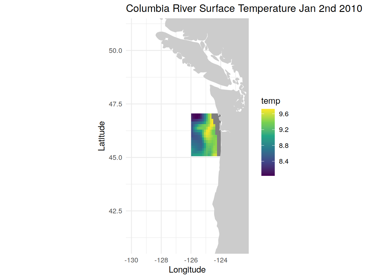

#converts time dimension to regular, rest in temp file
days_reg <- st_get_dimension_values(colriv_temp, "time") %>% ymd()
colriv_temp <- st_set_dimensions(colriv_temp, "time", values = days_reg)

#extract year-month
colriv_temp <- st_set_dimensions(colriv_temp, "time", values = format(
  days_reg,"%Y-%m"))

#turning data into dataframe and editing for use
colriv_temp <-colriv_temp %>%
  drop_units() %>% 
  as.data.frame(long = TRUE) %>% 
  select(-depth)

#creating new data frame with grouped month and the mean SST for each
colriv_monthly_2010_2015 <- colriv_temp %>% group_by(time) %>% 
  summarise(ColumbiaRiver_MeanMonthlySST = mean(temp, na.rm = TRUE))

#since this data includes the first data point of 2016 and we don't need
colriv_monthly_2010_2015 <- colriv_monthly_2010_2015 %>% slice(-n())


####################
#For San Francisco location
#opening specific nc file to get overview
# view_nc <- nc_open(paste0(path_ROMSv2RG_results,
#                      "SanFrancisco/SanFrancisco_2010-2015_control.nc"))
# 
# print(view_nc)

#filtering for just SST in 2x2deg box (36.5N-38.5N, 122.5W-124.5W), full time
sanfran_temp <- read_ncdf(paste0(path_ROMSv2RG_results,
                     "SanFrancisco/SanFrancisco_2010-2015_control.nc"),
           var = "temp",
           ncsub = cbind(start = c(33, 39, 1, 1), count = c(16, 16, 1, 1096)
             ),
           proxy = FALSE #need this on to override the proxy format
          )

No projection information found in nc file. 
 Coordinate variable units found to be degrees, 
 assuming WGS84 Lat/Lon.

#plotting specific time points to look at the selected region
sanfran_jan2016_temp <- sanfran_temp %>% 
  slice(time, 1096)

ggplot() +
 geom_stars(data = sanfran_jan2016_temp, aes(fill = temp)) +
  borders("world", colour = "gray80", fill = "gray80") +
  labs(title = "San Francisco Surface Temperature Jan 2nd 2016",
       x = "Longitude",
       y = "Latitude") +
  theme_minimal() + 
  scale_fill_viridis_c() +
  coord_quickmap(xlim = c(-127,-120), ylim = c(34, 42))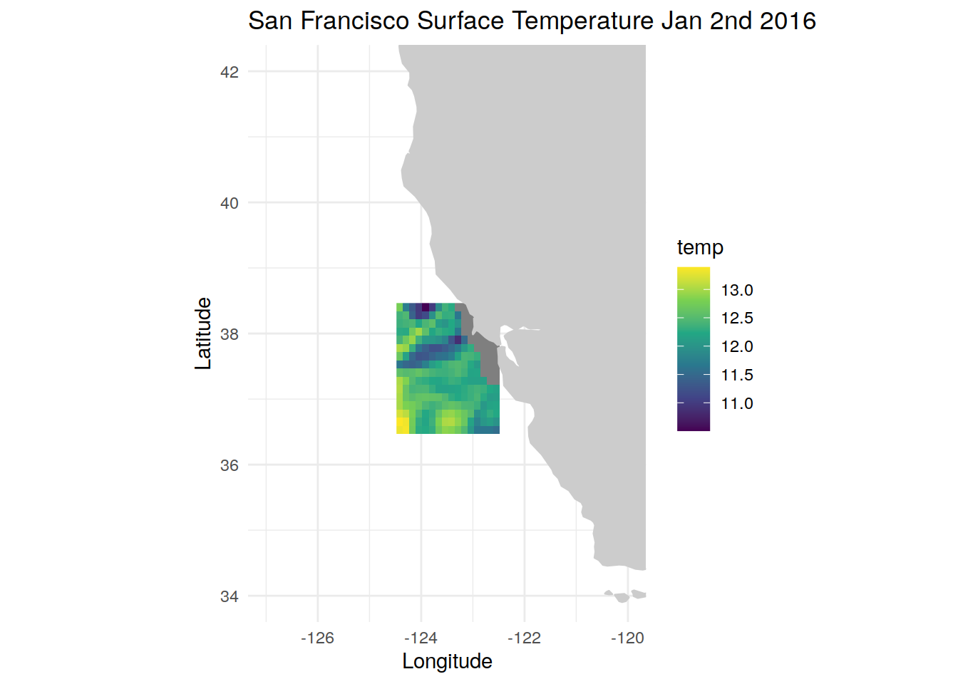

#converts time dimension to regular , rest in temp file
days_reg <- st_get_dimension_values(sanfran_temp, "time") %>% ymd()
sanfran_temp <- st_set_dimensions(sanfran_temp, "time", values = days_reg)

#extract year-month
sanfran_temp <- st_set_dimensions(sanfran_temp, "time", values = format(
  days_reg,"%Y-%m"))

#turning data into dataframe and editing for use
sanfran_temp <-sanfran_temp %>%
  drop_units() %>% 
  as.data.frame(long = TRUE) %>% 
  select(-depth)

#creating new data frame with grouped month and the mean SST for each
sanfran_monthly_2010_2015 <- sanfran_temp %>% group_by(time) %>% 
  summarise(SanFrancisco_MeanMonthlySST = mean(temp, na.rm = TRUE))

#since this data includes the first data point of 2016 and we don't need
sanfran_monthly_2010_2015 <- sanfran_monthly_2010_2015 %>% slice(-n())


####################
#For Huntington location
#opening specific nc file to get overview
# view_nc <- nc_open(paste0(path_ROMSv2RG_results,
#                      "Huntington/Huntington_2010-2015_control.nc"))
# 
# print(view_nc)

#filtering for just SST in 2x2deg box (32N-34N, 117W-119W), full time series
hunt_temp <- read_ncdf(paste0(path_ROMSv2RG_results,
                     "Huntington/Huntington_2010-2015_control.nc"),
           var = "temp",
           ncsub = cbind(start = c(50, 44, 1, 1), count = c(16, 16, 1, 1096)
             ),
           proxy = FALSE #need this on to override the proxy format
          )

No projection information found in nc file. 
 Coordinate variable units found to be degrees, 
 assuming WGS84 Lat/Lon.

#plotting the first time point to look at the selected region
hunt_jan2010_temp <- hunt_temp %>% 
  slice(time, 1)

ggplot() +
 geom_stars(data = hunt_jan2010_temp, aes(fill = temp)) +
  borders("world", colour = "gray80", fill = "gray80") +
  labs(title = "Huntington Surface Temperature Jan 2nd 2010",
       x = "Longitude",
       y = "Latitude") +
  theme_minimal() + 
  scale_fill_viridis_c() +
  coord_quickmap(xlim = c(-123,-115), ylim = c(26.5, 34.5))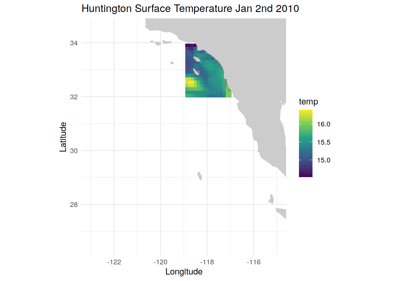

# #All 3 regions
# ggplot() +
#  geom_stars(data = hunt_jan2010_temp, aes(fill = temp)) +
#   geom_stars(data = sanfran_jan2010_temp, aes(fill = temp)) +
#   geom_stars(data = colriv_jan2010_temp, aes(fill = temp)) +
#   borders("world", colour = "gray80", fill = "gray80") +
#   labs(title = "CCS Surface Temperature Jan 2nd 2010",
#        x = "Longitude",
#        y = "Latitude") +
#   theme_minimal() + 
#   scale_fill_viridis_c() +
#   coord_quickmap(xlim = c(-130,-115), ylim = c(26.5, 49.5))

#converts time dimension to regular , rest in temp file
days_reg <- st_get_dimension_values(hunt_temp, "time") %>% ymd()
hunt_temp <- st_set_dimensions(hunt_temp, "time", values = days_reg)

#extract year-month
hunt_temp <- st_set_dimensions(hunt_temp, "time", values = format(
  days_reg,"%Y-%m"))

#turning data into dataframe and editing for use
hunt_temp <-hunt_temp %>%
  drop_units() %>% #see if i need this
  as.data.frame(long = TRUE) %>% 
  select(-depth)

#creating new data frame with grouped month and the mean SST for each
hunt_monthly_2010_2015 <- hunt_temp %>% group_by(time) %>% 
  summarise(Huntington_MeanMonthlySST = mean(temp, na.rm = TRUE))

#since this data includes the first data point of 2016 and we don't need
hunt_monthly_2010_2015 <- hunt_monthly_2010_2015 %>% slice(-n())


#####################
#For tropical 3.4 region: 5S->5N, 120W->170W
#opening specific nc file to get overview
# view_nc <- nc_open(paste0(path_ROMSv2RG_results,
#                      "regrid_2024_10/surface_temp_tropPacific/Control_2010_monthly_tropPacific.nc"))
# 
# print(view_nc)

#reading in all 6 years of monthly data and combining into 1 stars object
years <- 2010:2015
tropP_temp <- do.call(c, lapply(years, function(year) (
  read_ncdf(paste0(path_ROMSv2RG_results,
                   "regrid_2024_10/surface_temp_tropPacific/Control_", year, 
                   "_monthly_tropPacific.nc"),
           var = "temp",
           proxy = FALSE #need this on to override the proxy format
          ))))

No projection information found in nc file. 
 Coordinate variable units found to be degrees, 
 assuming WGS84 Lat/Lon.
No projection information found in nc file. 
 Coordinate variable units found to be degrees, 
 assuming WGS84 Lat/Lon.
No projection information found in nc file. 
 Coordinate variable units found to be degrees, 
 assuming WGS84 Lat/Lon.
No projection information found in nc file. 
 Coordinate variable units found to be degrees, 
 assuming WGS84 Lat/Lon.
No projection information found in nc file. 
 Coordinate variable units found to be degrees, 
 assuming WGS84 Lat/Lon.
No projection information found in nc file. 
 Coordinate variable units found to be degrees, 
 assuming WGS84 Lat/Lon.

#plotting the first time point to look at the selected region
tropP_jan2010_temp <- tropP_temp %>% 
  slice(time, 1)

ggplot() +
 geom_stars(data = tropP_jan2010_temp, aes(fill = temp)) +
  borders("world", colour = "gray80", fill = "gray80") +
  labs(title = "Tropical Pacific 3.4 Surface Temperature Jan 2nd 2010",
       x = "Longitude",
       y = "Latitude") +
  theme_minimal() + 
  scale_fill_viridis_c() +
  coord_quickmap(xlim = c(-175,-115), ylim = c(-10.5, 10.5))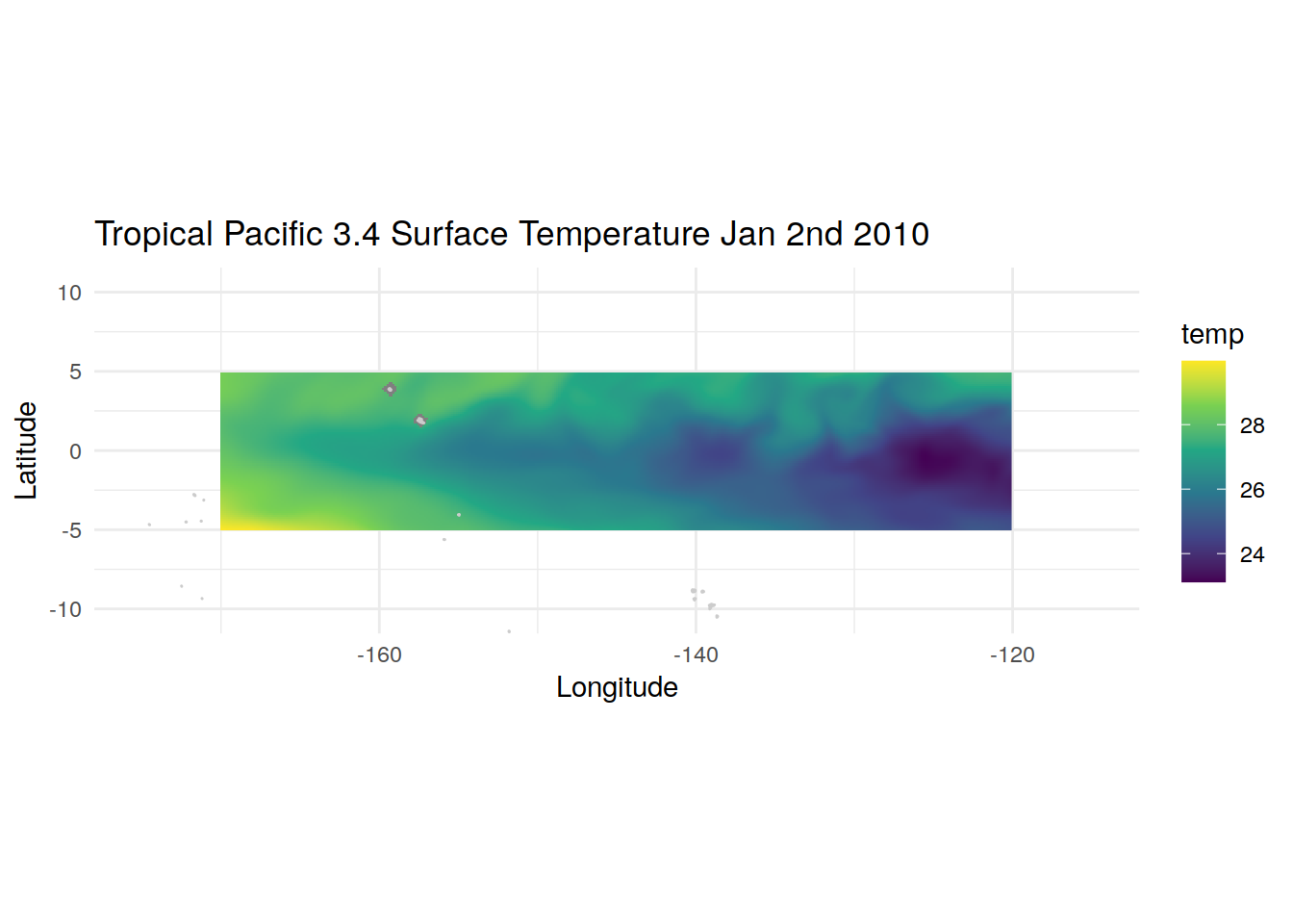

#converts time dimension to regular , rest in temp file
days_reg <- st_get_dimension_values(tropP_temp, "time")
tropP_temp <- st_set_dimensions(tropP_temp, "time", values = days_reg)

#extract year-month
tropP_temp <- st_set_dimensions(tropP_temp, "time", values = format(
  ymd_hms(days_reg),"%Y-%m"))


#turning data into dataframe and editing for use
tropP_temp <-tropP_temp %>%
  drop_units() %>% 
  as.data.frame(long = TRUE) %>% 
  select(-s_rho)

#creating new data frame with grouped month and the mean SST for each
tropP_monthly_2010_2015 <- tropP_temp %>% group_by(time) %>% 
  summarise(tropPacific_MeanMonthlySST = mean(temp, na.rm = TRUE))


#####################
#plotting all 4 time series of annual mean SST
p <- ggplot(data = tropP_monthly_2010_2015, 
       aes(x = time, y = tropPacific_MeanMonthlySST, group = 1)) + 
  geom_line(aes(color = "Tropical Pacific")) +
  geom_line(data = colriv_monthly_2010_2015, 
            aes(y = ColumbiaRiver_MeanMonthlySST, color = "Columbia River")) +
  geom_line(data = sanfran_monthly_2010_2015, 
            aes(y = SanFrancisco_MeanMonthlySST, color = "San Fransisco")) +
  geom_line(data = hunt_monthly_2010_2015, aes(y = Huntington_MeanMonthlySST,
                                               color = "Huntington")) +
  labs(title = "Monthly Mean SST", x = "Month", y = "Mean SST") +
  theme_minimal() +
  theme(axis.text.x = element_text(angle = 90, vjust = 0.5, hjust = 1))

####################
#30 year time series of historical monthly averages for all 4 locations
years_past <- 1979:2009
locations <- c("ColumbiaRiver", "Huntington", "SanFrancisco", "tropPacific")
annual_cycles <- list()
annual_monthly_SST_list <- list()

for (i in locations){
  #reading in all 30 years of data for each location into a stars object
  annual_cycles[[i]] <- do.call(c, lapply(years_past, function(year)(
    read_ncdf(paste0(path_ROMSv2RG_results,
                     "regrid_2024_10/1979-2009/pactcs30_", year, 
                     "_avg_", i, ".nc"),
              var = "temp",
              proxy = FALSE
  ))))
  #converting time dimensions, extracting year-month
  days_list <- st_get_dimension_values(annual_cycles[[i]], "time")
  annual_cycles[[i]] <- st_set_dimensions(annual_cycles[[i]], 
                                          "time", values = days_list)
  annual_cycles[[i]] <- st_set_dimensions(annual_cycles[[i]], "time", 
                        values = format(ymd_hms(days_list),"%Y-%m"))
  
  #converting each stars object into a dataframe and cleaning up
  annual_cycles[[i]] <- annual_cycles[[i]] %>% 
    drop_units() %>% 
    as.data.frame(long = TRUE) %>% 
    select(-s_rho)
  
  #creating a new data frame with the monthly averages over each region
  annual_monthly_SST_list[[i]] <- annual_cycles[[i]] %>% 
    group_by(time) %>% 
    summarise(mean_value = mean(temp, na.rm = TRUE), .groups = 'drop') %>% 
    rename(!!paste0(i, "_MeanMonthlySST") := mean_value)
  
}

No projection information found in nc file. 
 Coordinate variable units found to be degrees, 
 assuming WGS84 Lat/Lon.
No projection information found in nc file. 
 Coordinate variable units found to be degrees, 
 assuming WGS84 Lat/Lon.
No projection information found in nc file. 
 Coordinate variable units found to be degrees, 
 assuming WGS84 Lat/Lon.
No projection information found in nc file. 
 Coordinate variable units found to be degrees, 
 assuming WGS84 Lat/Lon.
No projection information found in nc file. 
 Coordinate variable units found to be degrees, 
 assuming WGS84 Lat/Lon.
No projection information found in nc file. 
 Coordinate variable units found to be degrees, 
 assuming WGS84 Lat/Lon.
No projection information found in nc file. 
 Coordinate variable units found to be degrees, 
 assuming WGS84 Lat/Lon.
No projection information found in nc file. 
 Coordinate variable units found to be degrees, 
 assuming WGS84 Lat/Lon.
No projection information found in nc file. 
 Coordinate variable units found to be degrees, 
 assuming WGS84 Lat/Lon.
No projection information found in nc file. 
 Coordinate variable units found to be degrees, 
 assuming WGS84 Lat/Lon.
No projection information found in nc file. 
 Coordinate variable units found to be degrees, 
 assuming WGS84 Lat/Lon.
No projection information found in nc file. 
 Coordinate variable units found to be degrees, 
 assuming WGS84 Lat/Lon.
No projection information found in nc file. 
 Coordinate variable units found to be degrees, 
 assuming WGS84 Lat/Lon.
No projection information found in nc file. 
 Coordinate variable units found to be degrees, 
 assuming WGS84 Lat/Lon.
No projection information found in nc file. 
 Coordinate variable units found to be degrees, 
 assuming WGS84 Lat/Lon.
No projection information found in nc file. 
 Coordinate variable units found to be degrees, 
 assuming WGS84 Lat/Lon.
No projection information found in nc file. 
 Coordinate variable units found to be degrees, 
 assuming WGS84 Lat/Lon.
No projection information found in nc file. 
 Coordinate variable units found to be degrees, 
 assuming WGS84 Lat/Lon.
No projection information found in nc file. 
 Coordinate variable units found to be degrees, 
 assuming WGS84 Lat/Lon.
No projection information found in nc file. 
 Coordinate variable units found to be degrees, 
 assuming WGS84 Lat/Lon.
No projection information found in nc file. 
 Coordinate variable units found to be degrees, 
 assuming WGS84 Lat/Lon.
No projection information found in nc file. 
 Coordinate variable units found to be degrees, 
 assuming WGS84 Lat/Lon.
No projection information found in nc file. 
 Coordinate variable units found to be degrees, 
 assuming WGS84 Lat/Lon.
No projection information found in nc file. 
 Coordinate variable units found to be degrees, 
 assuming WGS84 Lat/Lon.
No projection information found in nc file. 
 Coordinate variable units found to be degrees, 
 assuming WGS84 Lat/Lon.
No projection information found in nc file. 
 Coordinate variable units found to be degrees, 
 assuming WGS84 Lat/Lon.
No projection information found in nc file. 
 Coordinate variable units found to be degrees, 
 assuming WGS84 Lat/Lon.
No projection information found in nc file. 
 Coordinate variable units found to be degrees, 
 assuming WGS84 Lat/Lon.
No projection information found in nc file. 
 Coordinate variable units found to be degrees, 
 assuming WGS84 Lat/Lon.
No projection information found in nc file. 
 Coordinate variable units found to be degrees, 
 assuming WGS84 Lat/Lon.
No projection information found in nc file. 
 Coordinate variable units found to be degrees, 
 assuming WGS84 Lat/Lon.
No projection information found in nc file. 
 Coordinate variable units found to be degrees, 
 assuming WGS84 Lat/Lon.
No projection information found in nc file. 
 Coordinate variable units found to be degrees, 
 assuming WGS84 Lat/Lon.
No projection information found in nc file. 
 Coordinate variable units found to be degrees, 
 assuming WGS84 Lat/Lon.
No projection information found in nc file. 
 Coordinate variable units found to be degrees, 
 assuming WGS84 Lat/Lon.
No projection information found in nc file. 
 Coordinate variable units found to be degrees, 
 assuming WGS84 Lat/Lon.
No projection information found in nc file. 
 Coordinate variable units found to be degrees, 
 assuming WGS84 Lat/Lon.
No projection information found in nc file. 
 Coordinate variable units found to be degrees, 
 assuming WGS84 Lat/Lon.
No projection information found in nc file. 
 Coordinate variable units found to be degrees, 
 assuming WGS84 Lat/Lon.
No projection information found in nc file. 
 Coordinate variable units found to be degrees, 
 assuming WGS84 Lat/Lon.
No projection information found in nc file. 
 Coordinate variable units found to be degrees, 
 assuming WGS84 Lat/Lon.
No projection information found in nc file. 
 Coordinate variable units found to be degrees, 
 assuming WGS84 Lat/Lon.
No projection information found in nc file. 
 Coordinate variable units found to be degrees, 
 assuming WGS84 Lat/Lon.
No projection information found in nc file. 
 Coordinate variable units found to be degrees, 
 assuming WGS84 Lat/Lon.
No projection information found in nc file. 
 Coordinate variable units found to be degrees, 
 assuming WGS84 Lat/Lon.
No projection information found in nc file. 
 Coordinate variable units found to be degrees, 
 assuming WGS84 Lat/Lon.
No projection information found in nc file. 
 Coordinate variable units found to be degrees, 
 assuming WGS84 Lat/Lon.
No projection information found in nc file. 
 Coordinate variable units found to be degrees, 
 assuming WGS84 Lat/Lon.
No projection information found in nc file. 
 Coordinate variable units found to be degrees, 
 assuming WGS84 Lat/Lon.
No projection information found in nc file. 
 Coordinate variable units found to be degrees, 
 assuming WGS84 Lat/Lon.
No projection information found in nc file. 
 Coordinate variable units found to be degrees, 
 assuming WGS84 Lat/Lon.
No projection information found in nc file. 
 Coordinate variable units found to be degrees, 
 assuming WGS84 Lat/Lon.
No projection information found in nc file. 
 Coordinate variable units found to be degrees, 
 assuming WGS84 Lat/Lon.
No projection information found in nc file. 
 Coordinate variable units found to be degrees, 
 assuming WGS84 Lat/Lon.
No projection information found in nc file. 
 Coordinate variable units found to be degrees, 
 assuming WGS84 Lat/Lon.
No projection information found in nc file. 
 Coordinate variable units found to be degrees, 
 assuming WGS84 Lat/Lon.
No projection information found in nc file. 
 Coordinate variable units found to be degrees, 
 assuming WGS84 Lat/Lon.
No projection information found in nc file. 
 Coordinate variable units found to be degrees, 
 assuming WGS84 Lat/Lon.
No projection information found in nc file. 
 Coordinate variable units found to be degrees, 
 assuming WGS84 Lat/Lon.
No projection information found in nc file. 
 Coordinate variable units found to be degrees, 
 assuming WGS84 Lat/Lon.
No projection information found in nc file. 
 Coordinate variable units found to be degrees, 
 assuming WGS84 Lat/Lon.
No projection information found in nc file. 
 Coordinate variable units found to be degrees, 
 assuming WGS84 Lat/Lon.
No projection information found in nc file. 
 Coordinate variable units found to be degrees, 
 assuming WGS84 Lat/Lon.
No projection information found in nc file. 
 Coordinate variable units found to be degrees, 
 assuming WGS84 Lat/Lon.
No projection information found in nc file. 
 Coordinate variable units found to be degrees, 
 assuming WGS84 Lat/Lon.
No projection information found in nc file. 
 Coordinate variable units found to be degrees, 
 assuming WGS84 Lat/Lon.
No projection information found in nc file. 
 Coordinate variable units found to be degrees, 
 assuming WGS84 Lat/Lon.
No projection information found in nc file. 
 Coordinate variable units found to be degrees, 
 assuming WGS84 Lat/Lon.
No projection information found in nc file. 
 Coordinate variable units found to be degrees, 
 assuming WGS84 Lat/Lon.
No projection information found in nc file. 
 Coordinate variable units found to be degrees, 
 assuming WGS84 Lat/Lon.
No projection information found in nc file. 
 Coordinate variable units found to be degrees, 
 assuming WGS84 Lat/Lon.
No projection information found in nc file. 
 Coordinate variable units found to be degrees, 
 assuming WGS84 Lat/Lon.
No projection information found in nc file. 
 Coordinate variable units found to be degrees, 
 assuming WGS84 Lat/Lon.
No projection information found in nc file. 
 Coordinate variable units found to be degrees, 
 assuming WGS84 Lat/Lon.
No projection information found in nc file. 
 Coordinate variable units found to be degrees, 
 assuming WGS84 Lat/Lon.
No projection information found in nc file. 
 Coordinate variable units found to be degrees, 
 assuming WGS84 Lat/Lon.
No projection information found in nc file. 
 Coordinate variable units found to be degrees, 
 assuming WGS84 Lat/Lon.
No projection information found in nc file. 
 Coordinate variable units found to be degrees, 
 assuming WGS84 Lat/Lon.
No projection information found in nc file. 
 Coordinate variable units found to be degrees, 
 assuming WGS84 Lat/Lon.
No projection information found in nc file. 
 Coordinate variable units found to be degrees, 
 assuming WGS84 Lat/Lon.
No projection information found in nc file. 
 Coordinate variable units found to be degrees, 
 assuming WGS84 Lat/Lon.
No projection information found in nc file. 
 Coordinate variable units found to be degrees, 
 assuming WGS84 Lat/Lon.
No projection information found in nc file. 
 Coordinate variable units found to be degrees, 
 assuming WGS84 Lat/Lon.
No projection information found in nc file. 
 Coordinate variable units found to be degrees, 
 assuming WGS84 Lat/Lon.
No projection information found in nc file. 
 Coordinate variable units found to be degrees, 
 assuming WGS84 Lat/Lon.
No projection information found in nc file. 
 Coordinate variable units found to be degrees, 
 assuming WGS84 Lat/Lon.
No projection information found in nc file. 
 Coordinate variable units found to be degrees, 
 assuming WGS84 Lat/Lon.
No projection information found in nc file. 
 Coordinate variable units found to be degrees, 
 assuming WGS84 Lat/Lon.
No projection information found in nc file. 
 Coordinate variable units found to be degrees, 
 assuming WGS84 Lat/Lon.
No projection information found in nc file. 
 Coordinate variable units found to be degrees, 
 assuming WGS84 Lat/Lon.
No projection information found in nc file. 
 Coordinate variable units found to be degrees, 
 assuming WGS84 Lat/Lon.
No projection information found in nc file. 
 Coordinate variable units found to be degrees, 
 assuming WGS84 Lat/Lon.
No projection information found in nc file. 
 Coordinate variable units found to be degrees, 
 assuming WGS84 Lat/Lon.
No projection information found in nc file. 
 Coordinate variable units found to be degrees, 
 assuming WGS84 Lat/Lon.
No projection information found in nc file. 
 Coordinate variable units found to be degrees, 
 assuming WGS84 Lat/Lon.
No projection information found in nc file. 
 Coordinate variable units found to be degrees, 
 assuming WGS84 Lat/Lon.
No projection information found in nc file. 
 Coordinate variable units found to be degrees, 
 assuming WGS84 Lat/Lon.
No projection information found in nc file. 
 Coordinate variable units found to be degrees, 
 assuming WGS84 Lat/Lon.
No projection information found in nc file. 
 Coordinate variable units found to be degrees, 
 assuming WGS84 Lat/Lon.
No projection information found in nc file. 
 Coordinate variable units found to be degrees, 
 assuming WGS84 Lat/Lon.
No projection information found in nc file. 
 Coordinate variable units found to be degrees, 
 assuming WGS84 Lat/Lon.
No projection information found in nc file. 
 Coordinate variable units found to be degrees, 
 assuming WGS84 Lat/Lon.
No projection information found in nc file. 
 Coordinate variable units found to be degrees, 
 assuming WGS84 Lat/Lon.
No projection information found in nc file. 
 Coordinate variable units found to be degrees, 
 assuming WGS84 Lat/Lon.
No projection information found in nc file. 
 Coordinate variable units found to be degrees, 
 assuming WGS84 Lat/Lon.
No projection information found in nc file. 
 Coordinate variable units found to be degrees, 
 assuming WGS84 Lat/Lon.
No projection information found in nc file. 
 Coordinate variable units found to be degrees, 
 assuming WGS84 Lat/Lon.
No projection information found in nc file. 
 Coordinate variable units found to be degrees, 
 assuming WGS84 Lat/Lon.
No projection information found in nc file. 
 Coordinate variable units found to be degrees, 
 assuming WGS84 Lat/Lon.
No projection information found in nc file. 
 Coordinate variable units found to be degrees, 
 assuming WGS84 Lat/Lon.
No projection information found in nc file. 
 Coordinate variable units found to be degrees, 
 assuming WGS84 Lat/Lon.
No projection information found in nc file. 
 Coordinate variable units found to be degrees, 
 assuming WGS84 Lat/Lon.
No projection information found in nc file. 
 Coordinate variable units found to be degrees, 
 assuming WGS84 Lat/Lon.
No projection information found in nc file. 
 Coordinate variable units found to be degrees, 
 assuming WGS84 Lat/Lon.
No projection information found in nc file. 
 Coordinate variable units found to be degrees, 
 assuming WGS84 Lat/Lon.
No projection information found in nc file. 
 Coordinate variable units found to be degrees, 
 assuming WGS84 Lat/Lon.
No projection information found in nc file. 
 Coordinate variable units found to be degrees, 
 assuming WGS84 Lat/Lon.
No projection information found in nc file. 
 Coordinate variable units found to be degrees, 
 assuming WGS84 Lat/Lon.
No projection information found in nc file. 
 Coordinate variable units found to be degrees, 
 assuming WGS84 Lat/Lon.
No projection information found in nc file. 
 Coordinate variable units found to be degrees, 
 assuming WGS84 Lat/Lon.
No projection information found in nc file. 
 Coordinate variable units found to be degrees, 
 assuming WGS84 Lat/Lon.
No projection information found in nc file. 
 Coordinate variable units found to be degrees, 
 assuming WGS84 Lat/Lon.
No projection information found in nc file. 
 Coordinate variable units found to be degrees, 
 assuming WGS84 Lat/Lon.
No projection information found in nc file. 
 Coordinate variable units found to be degrees, 
 assuming WGS84 Lat/Lon.

#combining 30-year data into a single data frame + the 2010-2015 data
annual_monthly_sst <- reduce(annual_monthly_SST_list, left_join, by = "time")

full_2010_2015 <- list(colriv_monthly_2010_2015, hunt_monthly_2010_2015, 
                       sanfran_monthly_2010_2015,tropP_monthly_2010_2015) %>% 
  reduce(full_join, by = "time")

annual_monthly_sst_full <- bind_rows(annual_monthly_sst, full_2010_2015)

#computing the mean over the full period for each month at each location
monthly_mean_baseline <- annual_monthly_sst_full %>% 
  mutate(month = format(as.Date(paste0(time, "-01")), "%m")) %>% 
  group_by(month) %>% 
  summarise(
    ColumbiaRiver_basemonthlySST = mean(ColumbiaRiver_MeanMonthlySST, 
                                        na.rm = TRUE),
    Huntington_basemonthlySST = mean(Huntington_MeanMonthlySST, na.rm = TRUE),
    SanFrancisco_basemonthlySST = mean(SanFrancisco_MeanMonthlySST, na.rm = TRUE),
    tropPacific_basemonthlySST = mean(tropPacific_MeanMonthlySST, na.rm = TRUE),
    .groups = 'drop')


####################
#Calculating anomaly index values
#Extracting the month from the full time period and adding a column for it
annual_monthly_sst_full$month <- substr(annual_monthly_sst_full$time, 6, 7)

anomaly_SST_data <- merge(annual_monthly_sst_full, monthly_mean_baseline, 
                     by = "month") 

#calculate the anomaly for each location/month ie time series - base month mean
for (j in locations) {
  anomaly_col <- paste0(j, "_SST_anomaly")
  anomaly_SST_data <- anomaly_SST_data %>% 
    mutate(!!anomaly_col := .data[[paste0(j, "_MeanMonthlySST")]] - 
           .data[[paste0(j, "_basemonthlySST")]])
}

#reduce unneeded columns and sort chronologically
anomaly_SST <- anomaly_SST_data %>% 
  select(time, ColumbiaRiver_SST_anomaly, Huntington_SST_anomaly, 
         SanFrancisco_SST_anomaly, tropPacific_SST_anomaly) %>% 
  arrange(time)

#plot temperature anomalies
options(repr.plot.width = 50, repr.plot.height = 6) #not doing anything
ggplot(data = anomaly_SST, aes(x = time, group = 1)) + 
  geom_line(aes(y = tropPacific_SST_anomaly, color = "Tropical Pacific")) +
  geom_line(aes(y = ColumbiaRiver_SST_anomaly, color = "Columbia River")) +
  geom_line(aes(y = SanFrancisco_SST_anomaly, color = "San Francisco")) +
  geom_line(aes(y = Huntington_SST_anomaly, color = "Huntington")) +
  scale_x_discrete(breaks = anomaly_SST$time[seq(1, nrow(anomaly_SST), by = 12)]) +
  labs(title = "Monthly SST Anomalies", x = "Time", y = "SST Anomaly (degC)") +
  theme_minimal() +
  theme(axis.text.x = element_text(angle = 90, vjust = 0.5, hjust = 1))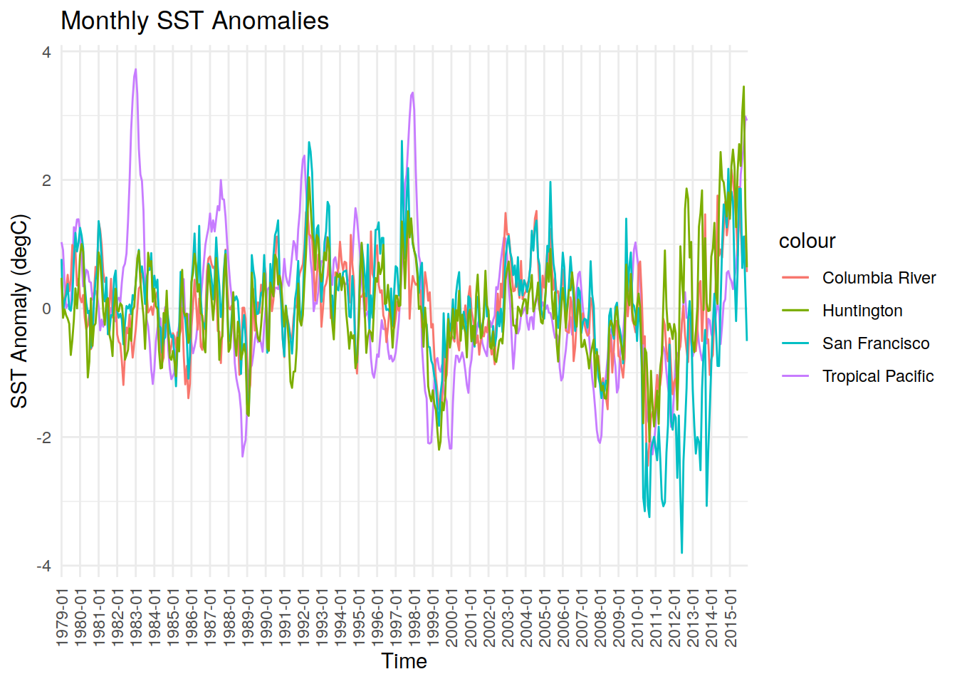

#Plotting subset
anomaly_SST <- anomaly_SST %>% 
  mutate(time = as.character(time))
subset_anomalySST <- anomaly_SST %>% 
  filter(time >= "2006-01")
ggplot(data = subset_anomalySST, aes(x = time, group = 1)) + 
  geom_line(aes(y = tropPacific_SST_anomaly, color = "Tropical Pacific")) +
  geom_line(aes(y = ColumbiaRiver_SST_anomaly, color = "Columbia River")) +
  geom_line(aes(y = SanFrancisco_SST_anomaly, color = "San Francisco")) +
  geom_line(aes(y = Huntington_SST_anomaly, color = "Huntington")) +
  scale_x_discrete(breaks = subset_anomalySST$time[seq(1, nrow(subset_anomalySST), by = 3)]) +
  labs(title = "Monthly SST Anomalies (2006 - 2015)", x = "Time", y = "SST Anomaly (degC)") +
  theme_minimal() +
  theme(axis.text.x = element_text(angle = 90, vjust = 0.5, hjust = 1))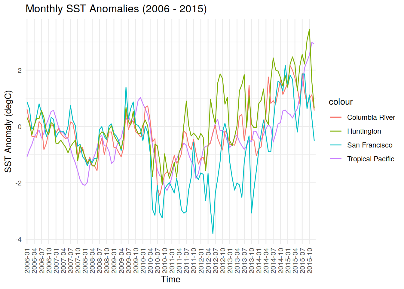

#####################
#Computing running annual mean ie mean temperature for one year starting that month
running_annual_mean_sst <- annual_monthly_sst_full
for (k in locations) {
  temp_col <- paste0(k, "_MeanMonthlySST")
  run_ann_mean_col <- paste0(k, "_SST_run_ann_mean")
  running_annual_mean_sst[[run_ann_mean_col]] <- NA #creates empty new column
  
  for (m in 1:(nrow(annual_monthly_sst_full) - 11)) { #will not calculate for 2015
    range <- annual_monthly_sst_full[[temp_col]][m:(m+11)] 
    #calculating and storing the running annual mean
    running_annual_mean_sst[[run_ann_mean_col]][m] <- mean(range, na.rm = TRUE)
    }
  }

ggplot(data = running_annual_mean_sst, aes(x = time, group = 1)) + 
  geom_line(aes(y = tropPacific_SST_run_ann_mean, color = "Tropical Pacific")) +
  geom_line(aes(y = ColumbiaRiver_SST_run_ann_mean, color = "Columbia River")) +
  geom_line(aes(y = SanFrancisco_SST_run_ann_mean, color = "San Francisco")) +
  geom_line(aes(y = Huntington_SST_run_ann_mean, color = "Huntington")) +
  scale_x_discrete(breaks = running_annual_mean_sst$time[
    seq(1, nrow(running_annual_mean_sst), by = 12)]) +
  labs(title = "Monthly SST Running Annual Mean", x = "Time", 
       y = "Running Annual Mean (degC)") +
  theme_minimal() +
  theme(axis.text.x = element_text(angle = 90, vjust = 0.5, hjust = 1))

Warning: Removed 11 rows containing missing values (`geom_line()`).
Removed 11 rows containing missing values (`geom_line()`).
Removed 11 rows containing missing values (`geom_line()`).
Removed 11 rows containing missing values (`geom_line()`).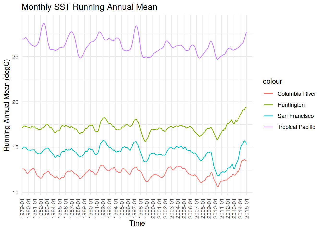

anomaly_sst_ram <- anomaly_SST
for (n in locations) {
  anom_col <- paste0(n, "_SST_anomaly")
  anom_ram_col <- paste0(n, "_sst_anom_ram")
  anomaly_sst_ram[[anom_ram_col]] <- NA #creates empty new column
  
  for (p in 1:(nrow(anomaly_SST) - 11)) { #will not calculate for 2015
    range <- anomaly_SST[[anom_col]][p:(p+11)] 
    #calculating and storing the running annual mean
    anomaly_sst_ram[[anom_ram_col]][p] <- mean(range, na.rm = TRUE)
    }
  }


ggplot(data = anomaly_sst_ram, aes(x = time, group = 1)) + 
  geom_line(aes(y = tropPacific_sst_anom_ram, color = "Tropical Pacific")) +
  geom_line(aes(y = ColumbiaRiver_sst_anom_ram, color = "Columbia River")) +
  geom_line(aes(y = SanFrancisco_sst_anom_ram, color = "San Francisco")) +
  geom_line(aes(y = Huntington_sst_anom_ram, color = "Huntington")) +
  scale_x_discrete(breaks = anomaly_sst_ram$time[
    seq(1, nrow(anomaly_sst_ram), by = 12)]) +
  labs(title = "SST Anomaly Running Annual Mean", x = "Time", 
       y = "SST Anomaly (degC)") +
  theme_minimal() +
  theme(axis.text.x = element_text(angle = 90, vjust = 0.5, hjust = 1))

Warning: Removed 11 rows containing missing values (`geom_line()`).
Removed 11 rows containing missing values (`geom_line()`).
Removed 11 rows containing missing values (`geom_line()`).
Removed 11 rows containing missing values (`geom_line()`).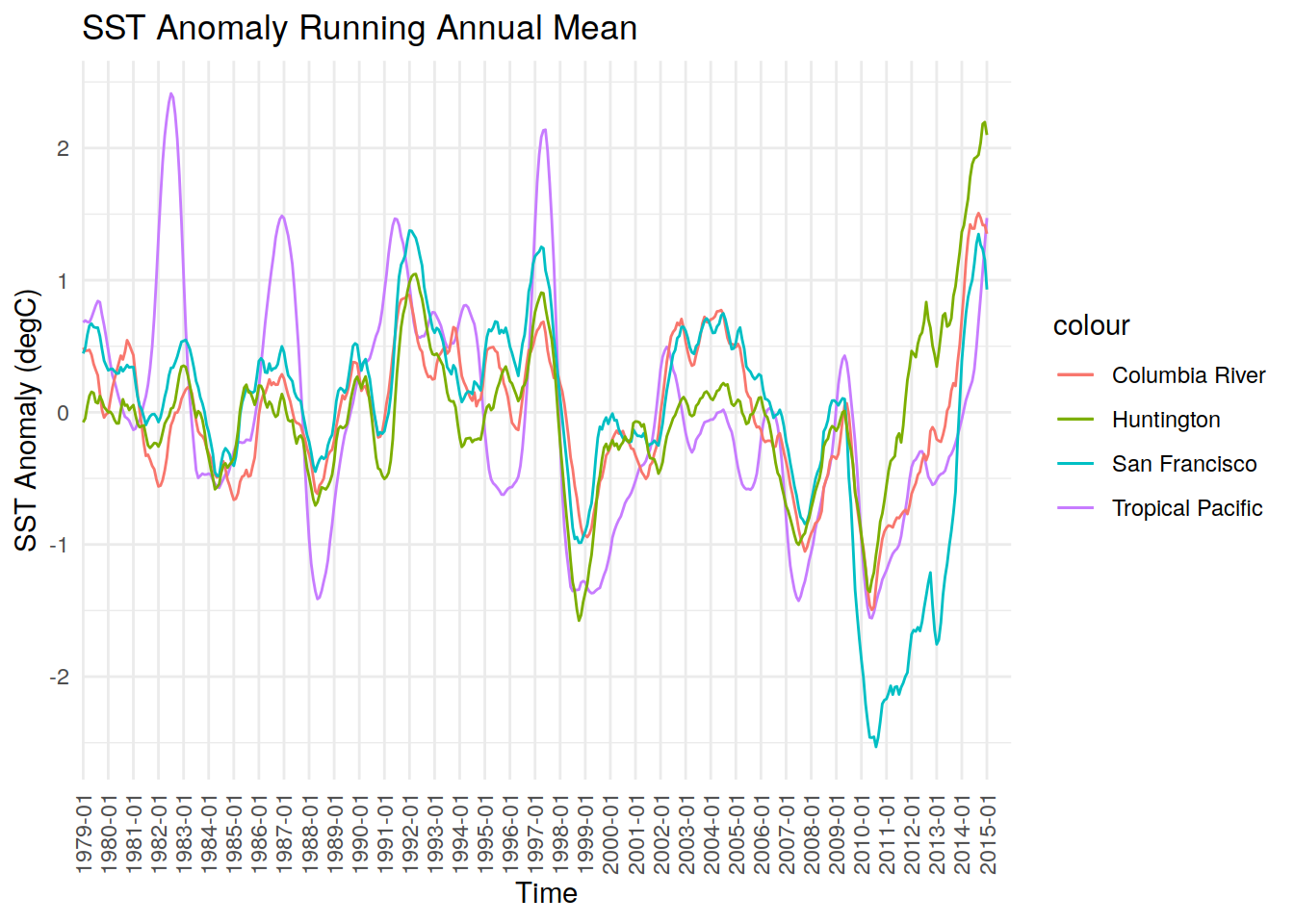

# #Plotting subset
# anomaly_sst_ram <- anomaly_sst_ram %>% 
#   mutate(time = as.character(time))
# subset_anomalySST_ram <- anomaly_sst_ram %>% 
#   filter(time >= "2010-01")
# ggplot(data = subset_anomalySST_ram, aes(x = time, group = 1)) + 
#   geom_line(aes(y = tropPacific_sst_anom_ram, color = "Tropical Pacific")) +
#   geom_line(aes(y = ColumbiaRiver_sst_anom_ram, color = "Columbia River")) +
#   geom_line(aes(y = SanFrancisco_sst_anom_ram, color = "San Francisco")) +
#   geom_line(aes(y = Huntington_sst_anom_ram, color = "Huntington")) +
#   scale_x_discrete(breaks = subset_anomalySST_ram$time[seq(1, nrow(subset_anomalySST_ram), by = 3)]) +
#   labs(title = "Monthly SST Anomaly RAM (2010 - 2014)", x = "Time", y = "SST Anomaly RAM (degC)") +
#   theme_minimal() +
#   theme(axis.text.x = element_text(angle = 90, vjust = 0.5, hjust = 1))


# #All 3 regions colors
# ggplot() +
#  geom_stars(data = tropP_jan2010_temp, aes(fill = "#C77CFF")) +
#   geom_stars(data = colriv_jan2010_temp, aes(fill = "#F8766D")) +
#   geom_stars(data = sanfran_jan2010_temp, aes(fill = "#00BFC4")) +
#   geom_stars(data = hunt_jan2010_temp, aes(fill = "#7CAE00")) +
#   borders("world", colour = "gray80", fill = "gray80") +
#   labs(title = "CCS Test Regions",
#        x = "Longitude",
#        y = "Latitude") +
#   theme_minimal() + 
#   scale_fill_identity(guide = "legend", 
#                       labels = c("Tropical Pacific", "Columbia River", "San Francisco", "Huntington"),
#                       breaks = c("#C77CFF", "#F8766D", "#00BFC4", "#7CAE00")) +
#   coord_quickmap(xlim = c(-170,-115), ylim = c(-10, 49.5))

######################
#Calculating correlation coefficients, pearson correlation test

cor.test(anomaly_SST$tropPacific_SST_anomaly, anomaly_SST$ColumbiaRiver_SST_anomaly)

    Pearson's product-moment correlation

data:  anomaly_SST$tropPacific_SST_anomaly and anomaly_SST$ColumbiaRiver_SST_anomaly
t = 10.15, df = 442, p-value < 2.2e-16
alternative hypothesis: true correlation is not equal to 0
95 percent confidence interval:
 0.3561311 0.5073177
sample estimates:
     cor 
0.434783 

cor.test(anomaly_SST$tropPacific_SST_anomaly, anomaly_SST$SanFrancisco_SST_anomaly)

    Pearson's product-moment correlation

data:  anomaly_SST$tropPacific_SST_anomaly and anomaly_SST$SanFrancisco_SST_anomaly
t = 10.538, df = 442, p-value < 2.2e-16
alternative hypothesis: true correlation is not equal to 0
95 percent confidence interval:
 0.3704769 0.5194885
sample estimates:
      cor 
0.4480896 

cor.test(anomaly_SST$tropPacific_SST_anomaly, anomaly_SST$Huntington_SST_anomaly)

    Pearson's product-moment correlation

data:  anomaly_SST$tropPacific_SST_anomaly and anomaly_SST$Huntington_SST_anomaly
t = 10.131, df = 442, p-value < 2.2e-16
alternative hypothesis: true correlation is not equal to 0
95 percent confidence interval:
 0.3554160 0.5067094
sample estimates:
      cor 
0.4341188 

cor.test(running_annual_mean_sst$tropPacific_SST_run_ann_mean,
         running_annual_mean_sst$ColumbiaRiver_SST_run_ann_mean)

    Pearson's product-moment correlation

data:  running_annual_mean_sst$tropPacific_SST_run_ann_mean and running_annual_mean_sst$ColumbiaRiver_SST_run_ann_mean
t = 15.188, df = 431, p-value < 2.2e-16
alternative hypothesis: true correlation is not equal to 0
95 percent confidence interval:
 0.5254327 0.6485840
sample estimates:
      cor 
0.5904345 

cor.test(running_annual_mean_sst$tropPacific_SST_run_ann_mean,
         running_annual_mean_sst$SanFrancisco_SST_run_ann_mean)

    Pearson's product-moment correlation

data:  running_annual_mean_sst$tropPacific_SST_run_ann_mean and running_annual_mean_sst$SanFrancisco_SST_run_ann_mean
t = 15.877, df = 431, p-value < 2.2e-16
alternative hypothesis: true correlation is not equal to 0
95 percent confidence interval:
 0.5444195 0.6637299
sample estimates:
      cor 
0.6074898 

cor.test(running_annual_mean_sst$tropPacific_SST_run_ann_mean,
         running_annual_mean_sst$Huntington_SST_run_ann_mean)

    Pearson's product-moment correlation

data:  running_annual_mean_sst$tropPacific_SST_run_ann_mean and running_annual_mean_sst$Huntington_SST_run_ann_mean
t = 12.883, df = 431, p-value < 2.2e-16
alternative hypothesis: true correlation is not equal to 0
95 percent confidence interval:
 0.4556806 0.5920925
sample estimates:
      cor 
0.5272757 

cor.test(subset_anomalySST$tropPacific_SST_anomaly,
         subset_anomalySST$ColumbiaRiver_SST_anomaly)

    Pearson's product-moment correlation

data:  subset_anomalySST$tropPacific_SST_anomaly and subset_anomalySST$ColumbiaRiver_SST_anomaly
t = 9.8751, df = 118, p-value < 2.2e-16
alternative hypothesis: true correlation is not equal to 0
95 percent confidence interval:
 0.5610752 0.7602463
sample estimates:
      cor 
0.6726678 

cor.test(subset_anomalySST$tropPacific_SST_anomaly,
         subset_anomalySST$SanFrancisco_SST_anomaly)

    Pearson's product-moment correlation

data:  subset_anomalySST$tropPacific_SST_anomaly and subset_anomalySST$SanFrancisco_SST_anomaly
t = 6.7299, df = 118, p-value = 6.467e-10
alternative hypothesis: true correlation is not equal to 0
95 percent confidence interval:
 0.3836302 0.6450105
sample estimates:
      cor 
0.5266573 

cor.test(subset_anomalySST$tropPacific_SST_anomaly,
         subset_anomalySST$Huntington_SST_anomaly)

    Pearson's product-moment correlation

data:  subset_anomalySST$tropPacific_SST_anomaly and subset_anomalySST$Huntington_SST_anomaly
t = 9.3118, df = 118, p-value = 8.526e-16
alternative hypothesis: true correlation is not equal to 0
95 percent confidence interval:
 0.5338603 0.7433504
sample estimates:
      cor 
0.6508243 

cor.test(anomaly_sst_ram$tropPacific_sst_anom_ram,
         anomaly_sst_ram$ColumbiaRiver_sst_anom_ram)

    Pearson's product-moment correlation

data:  anomaly_sst_ram$tropPacific_sst_anom_ram and anomaly_sst_ram$ColumbiaRiver_sst_anom_ram
t = 15.188, df = 431, p-value < 2.2e-16
alternative hypothesis: true correlation is not equal to 0
95 percent confidence interval:
 0.5254327 0.6485840
sample estimates:
      cor 
0.5904345 

cor.test(anomaly_sst_ram$tropPacific_sst_anom_ram,
         anomaly_sst_ram$SanFrancisco_sst_anom_ram)

    Pearson's product-moment correlation

data:  anomaly_sst_ram$tropPacific_sst_anom_ram and anomaly_sst_ram$SanFrancisco_sst_anom_ram
t = 15.877, df = 431, p-value < 2.2e-16
alternative hypothesis: true correlation is not equal to 0
95 percent confidence interval:
 0.5444195 0.6637299
sample estimates:
      cor 
0.6074898 

cor.test(anomaly_sst_ram$tropPacific_sst_anom_ram,
         anomaly_sst_ram$Huntington_sst_anom_ram)

    Pearson's product-moment correlation

data:  anomaly_sst_ram$tropPacific_sst_anom_ram and anomaly_sst_ram$Huntington_sst_anom_ram
t = 12.883, df = 431, p-value < 2.2e-16
alternative hypothesis: true correlation is not equal to 0
95 percent confidence interval:
 0.4556806 0.5920925
sample estimates:
      cor 
0.5272757 

vhjgvj

Session information

sessionInfo()

R version 4.2.2 (2022-10-31)
Platform: x86_64-pc-linux-gnu (64-bit)
Running under: openSUSE Leap 15.5

Matrix products: default
BLAS:   /usr/local/R-4.2.2/lib64/R/lib/libRblas.so
LAPACK: /usr/local/R-4.2.2/lib64/R/lib/libRlapack.so

locale:
 [1] LC_CTYPE=en_US.UTF-8       LC_NUMERIC=C              
 [3] LC_TIME=en_US.UTF-8        LC_COLLATE=en_US.UTF-8    
 [5] LC_MONETARY=en_US.UTF-8    LC_MESSAGES=en_US.UTF-8   
 [7] LC_PAPER=en_US.UTF-8       LC_NAME=C                 
 [9] LC_ADDRESS=C               LC_TELEPHONE=C            
[11] LC_MEASUREMENT=en_US.UTF-8 LC_IDENTIFICATION=C       

attached base packages:
[1] stats     graphics  grDevices utils     datasets  methods   base     

other attached packages:
 [1] units_0.8-0      lubridate_1.9.0  timechange_0.1.1 forcats_0.5.2   
 [5] stringr_1.5.0    dplyr_1.1.3      purrr_1.0.2      readr_2.1.3     
 [9] tidyr_1.3.0      tibble_3.2.1     ggplot2_3.4.4    tidyverse_1.3.2 
[13] stars_0.6-0      sf_1.0-9         abind_1.4-5      ncdf4_1.19      
[17] workflowr_1.7.0 

loaded via a namespace (and not attached):
 [1] fs_1.5.2            httr_1.4.4          rprojroot_2.0.3    
 [4] tools_4.2.2         backports_1.4.1     bslib_0.4.1        
 [7] utf8_1.2.2          R6_2.5.1            KernSmooth_2.23-20 
[10] DBI_1.1.3           colorspace_2.0-3    withr_2.5.0        
[13] tidyselect_1.2.0    processx_3.8.0      compiler_4.2.2     
[16] git2r_0.30.1        cli_3.6.1           rvest_1.0.3        
[19] RNetCDF_2.6-1       xml2_1.3.3          labeling_0.4.2     
[22] sass_0.4.4          scales_1.2.1        classInt_0.4-8     
[25] callr_3.7.3         proxy_0.4-27        digest_0.6.30      
[28] rmarkdown_2.18      pkgconfig_2.0.3     htmltools_0.5.3    
[31] highr_0.9           dbplyr_2.2.1        fastmap_1.1.0      
[34] maps_3.4.1          rlang_1.1.1         readxl_1.4.1       
[37] rstudioapi_0.15.0   PCICt_0.5-4.3       jquerylib_0.1.4    
[40] generics_0.1.3      farver_2.1.1        jsonlite_1.8.3     
[43] googlesheets4_1.0.1 magrittr_2.0.3      ncmeta_0.3.5       
[46] Rcpp_1.0.10         munsell_0.5.0       fansi_1.0.3        
[49] lifecycle_1.0.3     stringi_1.7.8       whisker_0.4        
[52] yaml_2.3.6          grid_4.2.2          parallel_4.2.2     
[55] promises_1.2.0.1    crayon_1.5.2        haven_2.5.1        
[58] hms_1.1.2           knitr_1.41          ps_1.7.2           
[61] pillar_1.9.0        reprex_2.0.2        glue_1.6.2         
[64] evaluate_0.18       getPass_0.2-2       modelr_0.1.10      
[67] vctrs_0.6.4         tzdb_0.3.0          httpuv_1.6.6       
[70] cellranger_1.1.0    gtable_0.3.1        assertthat_0.2.1   
[73] cachem_1.0.6        xfun_0.35           lwgeom_0.2-10      
[76] broom_1.0.5         e1071_1.7-12        later_1.3.0        
[79] class_7.3-20        googledrive_2.0.0   viridisLite_0.4.1  
[82] gargle_1.2.1        ellipsis_0.3.2