Regrid Checks and Column Integrated Plots
Victoria Froh
03 February, 2025
Last updated: 2025-02-03
Checks: 7 0
Knit directory: oae_ccs_roms/
This reproducible R Markdown analysis was created with workflowr (version 1.7.1). The Checks tab describes the reproducibility checks that were applied when the results were created. The Past versions tab lists the development history.
Great! Since the R Markdown file has been committed to the Git repository, you know the exact version of the code that produced these results.
Great job! The global environment was empty. Objects defined in the global environment can affect the analysis in your R Markdown file in unknown ways. For reproduciblity it’s best to always run the code in an empty environment.
The command set.seed(20240919) was run prior to running
the code in the R Markdown file. Setting a seed ensures that any results
that rely on randomness, e.g. subsampling or permutations, are
reproducible.
Great job! Recording the operating system, R version, and package versions is critical for reproducibility.
Nice! There were no cached chunks for this analysis, so you can be confident that you successfully produced the results during this run.
Great job! Using relative paths to the files within your workflowr project makes it easier to run your code on other machines.
Great! You are using Git for version control. Tracking code development and connecting the code version to the results is critical for reproducibility.
The results in this page were generated with repository version 639b38d. See the Past versions tab to see a history of the changes made to the R Markdown and HTML files.
Note that you need to be careful to ensure that all relevant files for
the analysis have been committed to Git prior to generating the results
(you can use wflow_publish or
wflow_git_commit). workflowr only checks the R Markdown
file, but you know if there are other scripts or data files that it
depends on. Below is the status of the Git repository when the results
were generated:
Ignored files:
    Ignored:    .Rhistory
    Ignored:    .Rproj.user/

Untracked files:
    Untracked:  code/read_data.Rmd
    Untracked:  oae_ccs_roms.Rproj.RData

Unstaged changes:
    Modified:   analysis/_site.yml
    Deleted:    analysis/read_data.Rmd
    Modified:   code/Workflowr_project_managment.R
    Modified:   code/regrid_cdr_eff_molar.R
    Modified:   code/regrid_dTA_dDIC.R
Note that any generated files, e.g. HTML, png, CSS, etc., are not included in this status report because it is ok for generated content to have uncommitted changes.
These are the previous versions of the repository in which changes were
made to the R Markdown (analysis/column_int_plots.Rmd) and
HTML (docs/column_int_plots.html) files. If you’ve
configured a remote Git repository (see ?wflow_git_remote),
click on the hyperlinks in the table below to view the files as they
were in that past version.
| File | Version | Author | Date | Message |
|---|---|---|---|---|
| Rmd | 639b38d | vgfroh | 2025-02-03 | Column integrated plots and hovmoeller plots completed |
Introduction
- Checking regrid subregion
- Verifying scope of dTA in regrid
- Column-integrated dTA maps
#loading packages
library(tidyverse)
library(data.table)
library(arrow)
library(scales)

# Path to intermediate computation outputs
path_outputs <- "/net/sea/work/vifroh/oae_ccs_roms_data/regrid_2/"

# Path to save practice plots when working on them
path_plots <- "/net/sea/work/vifroh/test_plots/"

# loading in dTA conc data to make a surface plot/columnint
lanina_dTA_conc <- read_feather(
  paste0(path_outputs,"lanina_dTA_concdataRG2.feather"))

# loading in dTA full integration data for competency check
lanina_dTA_int<- read_feather(
  paste0(path_outputs,"lanina_CDReff_intRG2.feather"))

# loading in dTA sum original grid data for competency check
lanina_intdata_ogs <- read_feather(
  "/net/sea/work/vifroh/oae_ccs_roms_data/regrid/lanina_dTAint_comparegrids.feather")
Looking at the boundaries of the regridded subregion
# filtering dTA conc data to make a surface plot
surface_data <- lanina_dTA_conc[depth == 0 & time == "1998-09"]

# Convert lat and lon to numeric
surface_data$lat <- as.numeric(surface_data$lat)
surface_data$lon <- as.numeric(surface_data$lon)

# # Convert longitude to -180 to 180 range
# surface_data$lon <- surface_data$lon - 360

# Define the bounding box for the plot
lat_range <- range(surface_data$lat, na.rm = TRUE)
lon_range <- range(surface_data$lon, na.rm = TRUE)

# plotting surface map
ggplot() +
  geom_polygon(data = map_data("world"), aes(x = long, y = lat, group = group),
               fill = "lightgray", color = "white") +
  geom_raster(data = surface_data, aes(x = lon, y = lat, fill = dTA)) +
  scale_fill_viridis_c() +  # Change the color scale to suit your data
  theme_minimal() +
  coord_fixed(xlim = c(lon_range[1] - 2, lon_range[2] + 2),
              ylim = c(lat_range[1] - 2, lat_range[2] + 2)) +
  theme(
    axis.text.x = element_text(angle = 90, hjust = 1, vjust = 0.5, size = 8),
    axis.text.y = element_text(size = 8),
    axis.ticks = element_line(size = 0.5),
    panel.grid = element_blank()
  ) +
  labs(title = "Subset Domain (La Niña, September 1998)",
       x = "Longitude",
       y = "Latitude",
       fill = "dTA (mmol/m^3)")
Warning: The `size` argument of `element_line()` is deprecated as of ggplot2 3.4.0.
ℹ Please use the `linewidth` argument instead.
This warning is displayed once every 8 hours.
Call `lifecycle::last_lifecycle_warnings()` to see where this warning was
generated.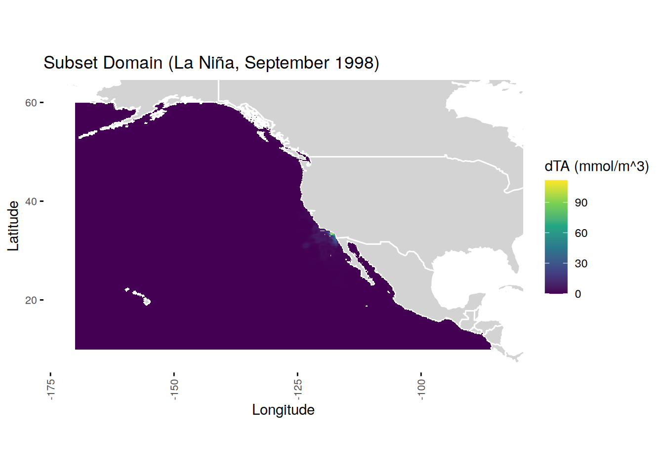
# save plot
ggsave(paste0(path_plots, "regrid_domainRG2.png"), plot = last_plot(),
       width = 8, height = 6, dpi = 300)

rm(surface_data)
gc()
used (Mb) gc trigger (Mb) max used (Mb)
Ncells 1657574 88.6 3217118 171.9 2798428 149.5
Vcells 3148545860 24021.5 4533694348 34589.4 3215779056 24534.5Checking the alkalinity containment within the regridded subregion over the time series
# using full integrated data from cdr_eff_molar file
setDT(lanina_dTA_int)

# combine with original dTA sum data to compare; subtracting regrid from original
lanina_dTAint_compare <- merge(lanina_intdata_ogs, lanina_dTA_int[, .(time, dTA_sum_rg2 = dTA_sum)],
                          by = "time", all.x = FALSE) %>%
  .[, dTA_dif_rg2 := dTA_sum_og - dTA_sum_rg2] %>%
  .[, frac_miss_rg2 := dTA_dif_rg2 / dTA_sum_og]

# # save data file
# write_feather(lanina_dTAint_compare, paste0(path_outputs,
#                                       "lanina_dTAint_comparegridsRG2.feather"))

rm(lanina_dTAint_compare, lanina_intdata_og)
Warning in rm(lanina_dTAint_compare, lanina_intdata_og): object
'lanina_intdata_og' not foundgc() used (Mb) gc trigger (Mb) max used (Mb)
Ncells 1666362 89.0 3217118 171.9 2798428 149.5
Vcells 3147534806 24013.8 4533694348 34589.4 3215779056 24534.5Column integrated plots of added alkalinity to check lateral movement during the time series
# using conc data then multiplied by depth bin size so have mmol/m^2
setDT(lanina_dTA_conc)
lanina_dTA_conc$depth <- as.numeric(lanina_dTA_conc$depth)
lanina_dTA_conc <-
  lanina_dTA_conc[, thickness :=
                    ifelse(depth == 0, 2.5,
                           ifelse(depth < 80, 5,
                                  ifelse(depth == 80, 7.5,
                                         ifelse(depth < 100, 10,
                                                ifelse(depth == 100, 15,
                                                       ifelse(depth < 300, 20,
                                                              10
                                                       ))))))]
lanina_dTA_conc <- lanina_dTA_conc[, dTA_m2 := dTA * thickness] %>%  # units now moles/m2
      .[, dDIC_m2 := dDIC * thickness]

# grouping by lat/lon and integrating vertically
lanina_dTA_columnint<- lanina_dTA_conc[, .(dTA_column = sum(dTA_m2, na.rm = TRUE)),
                                      by = c("lat", "lon", "time")]


# Convert lat, lon, Alk to numeric
lanina_dTA_columnint$lat <- as.numeric(lanina_dTA_columnint$lat)
lanina_dTA_columnint$lon <- as.numeric(lanina_dTA_columnint$lon)
lanina_dTA_columnint$dTA_column <- as.numeric(lanina_dTA_columnint$dTA_column)

# filter by time to create a timestop plot
surface_data <- lanina_dTA_columnint[time == "1999-06"]

# # Convert longitude to -180 to 180 range
# surface_data$lon <- surface_data$lon - 360

# plotting surface map
ggplot() +
  # geom_polygon(data = map_data("world"), aes(x = long, y = lat, group = group),
  #              fill = "lightgray", color = "white") +
  geom_raster(data = surface_data, aes(x = lon, y = lat, fill = dTA_column)) +
  scale_fill_viridis_c() +  # Change the color scale to suit your data
  theme_minimal() +
  coord_fixed() +
  scale_x_continuous(breaks = seq(-170, -85, by = 10)) +
  scale_y_continuous(breaks = seq(10, 60, by = 10)) +
  labs(title = "Vertically Integrated dTA (La Niña, June 1999)",
       x = "Longitude",
       y = "Latitude",
       fill = "dTA (mmol/m^2)")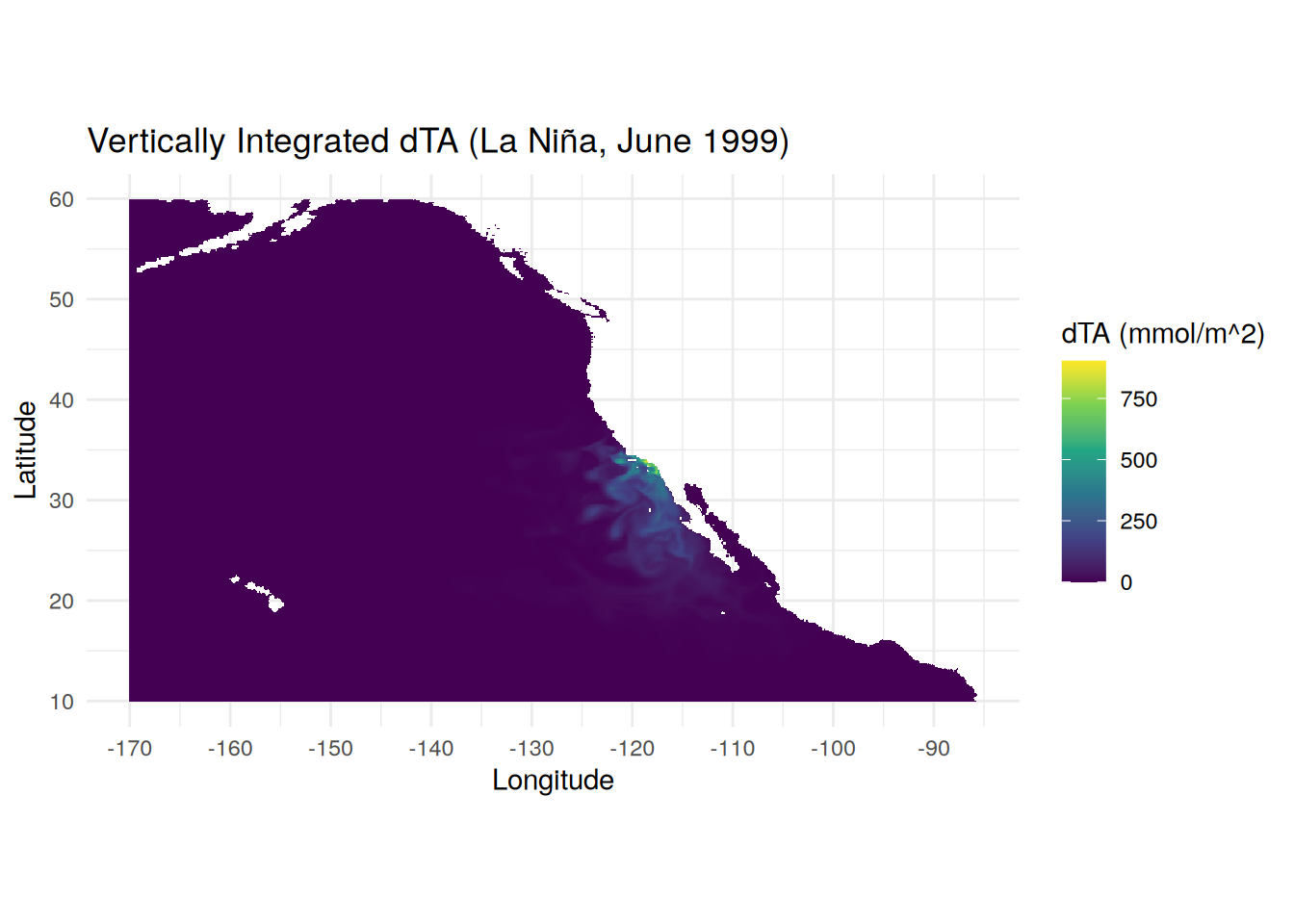
# save plot
ggsave(paste0(path_plots, "lanina_columnint_Jun1999.png"), plot = last_plot(),
       width = 8, height = 6, dpi = 300)

# # save column integrated data
# write_feather(lanina_dTA_columnint, paste0(path_outputs,
#                                       "lanina_columnintRG2.feather"))
# write_feather(neutral_dTA_columnint, paste0(path_outputs,
#                                        "neutral_columnintRG2.feather"))
# write_feather(elnino_dTA_columnint, paste0(path_outputs,
#                                       "elnino_columnintRG2.feather"))

rm(lanina_dTA_columnint, surface_data, lanina_dTA_conc)
gc()
used (Mb) gc trigger (Mb) max used (Mb)
Ncells 1676490 89.6 3217118 171.9 3217118 171.9
Vcells 4179417 31.9 8052609881 61436.6 9725788468 74201.9
sessionInfo()R version 4.4.2 (2024-10-31)
Platform: x86_64-pc-linux-gnu
Running under: openSUSE Leap 15.6
Matrix products: default
BLAS/LAPACK: /usr/local/OpenBLAS-0.3.28/lib/libopenblas_haswellp-r0.3.28.so; LAPACK version 3.12.0
locale:
[1] LC_CTYPE=en_US.UTF-8 LC_NUMERIC=C
[3] LC_TIME=en_US.UTF-8 LC_COLLATE=en_US.UTF-8
[5] LC_MONETARY=en_US.UTF-8 LC_MESSAGES=en_US.UTF-8
[7] LC_PAPER=en_US.UTF-8 LC_NAME=C
[9] LC_ADDRESS=C LC_TELEPHONE=C
[11] LC_MEASUREMENT=en_US.UTF-8 LC_IDENTIFICATION=C
time zone: Europe/Zurich
tzcode source: system (glibc)
attached base packages:
[1] stats graphics grDevices utils datasets methods base
other attached packages:
[1] scales_1.3.0 arrow_18.1.0.1 data.table_1.16.2 lubridate_1.9.3
[5] forcats_1.0.0 stringr_1.5.1 dplyr_1.1.4 purrr_1.0.2
[9] readr_2.1.5 tidyr_1.3.1 tibble_3.2.1 ggplot2_3.5.1
[13] tidyverse_2.0.0 workflowr_1.7.1
loaded via a namespace (and not attached):
[1] gtable_0.3.6 xfun_0.49 bslib_0.8.0 processx_3.8.4
[5] callr_3.7.6 tzdb_0.4.0 vctrs_0.6.5 tools_4.4.2
[9] ps_1.8.1 generics_0.1.3 fansi_1.0.6 pkgconfig_2.0.3
[13] assertthat_0.2.1 lifecycle_1.0.4 compiler_4.4.2 farver_2.1.2
[17] git2r_0.35.0 textshaping_0.4.0 munsell_0.5.1 getPass_0.2-4
[21] httpuv_1.6.15 htmltools_0.5.8.1 maps_3.4.2.1 sass_0.4.9
[25] yaml_2.3.10 crayon_1.5.3 later_1.4.1 pillar_1.9.0
[29] jquerylib_0.1.4 whisker_0.4.1 cachem_1.1.0 tidyselect_1.2.1
[33] digest_0.6.37 stringi_1.8.4 labeling_0.4.3 rprojroot_2.0.4
[37] fastmap_1.2.0 grid_4.4.2 colorspace_2.1-1 cli_3.6.3
[41] magrittr_2.0.3 utf8_1.2.4 withr_3.0.2 promises_1.3.2
[45] bit64_4.5.2 timechange_0.3.0 rmarkdown_2.29 httr_1.4.7
[49] bit_4.5.0 ragg_1.3.3 hms_1.1.3 evaluate_1.0.1
[53] knitr_1.49 viridisLite_0.4.2 rlang_1.1.4 Rcpp_1.0.13-1
[57] glue_1.8.0 rstudioapi_0.17.1 jsonlite_1.8.9 R6_2.5.1
[61] systemfonts_1.1.0 fs_1.6.5