1. Above-ground biomass

Data summary
Biomass variable
Total biomass

Last updated: 2021-04-08

Checks: 7 0

Knit directory: RainDrop_biodiversity/

This reproducible R Markdown analysis was created with workflowr (version 1.6.2). The Checks tab describes the reproducibility checks that were applied when the results were created. The Past versions tab lists the development history.

R Markdown file: up-to-date

Great! Since the R Markdown file has been committed to the Git repository, you know the exact version of the code that produced these results.

Environment: empty

Great job! The global environment was empty. Objects defined in the global environment can affect the analysis in your R Markdown file in unknown ways. For reproduciblity it’s best to always run the code in an empty environment.

Seed: set.seed(20210406)

The command set.seed(20210406) was run prior to running the code in the R Markdown file. Setting a seed ensures that any results that rely on randomness, e.g. subsampling or permutations, are reproducible.

Session information: recorded

Great job! Recording the operating system, R version, and package versions is critical for reproducibility.

Cache: none

Nice! There were no cached chunks for this analysis, so you can be confident that you successfully produced the results during this run.

File paths: relative

Great job! Using relative paths to the files within your workflowr project makes it easier to run your code on other machines.

Repository version: f8308af

Great! You are using Git for version control. Tracking code development and connecting the code version to the results is critical for reproducibility.

The results in this page were generated with repository version f8308af. See the Past versions tab to see a history of the changes made to the R Markdown and HTML files.

Note that you need to be careful to ensure that all relevant files for the analysis have been committed to Git prior to generating the results (you can use wflow_publish or wflow_git_commit). workflowr only checks the R Markdown file, but you know if there are other scripts or data files that it depends on. Below is the status of the Git repository when the results were generated:


Ignored files:
    Ignored:    .Rhistory
    Ignored:    .Rproj.user/

Unstaged changes:
    Deleted:    analysis/about.Rmd

Note that any generated files, e.g. HTML, png, CSS, etc., are not included in this status report because it is ok for generated content to have uncommitted changes.

These are the previous versions of the repository in which changes were made to the R Markdown (analysis/exploratory_analysis.Rmd) and HTML (docs/exploratory_analysis.html) files. If you’ve configured a remote Git repository (see ?wflow_git_remote), click on the hyperlinks in the table below to view the files as they were in that past version.

File	Version	Author	Date	Message
Rmd	f8308af	jjackson-eco	2021-04-08	exploration for biomass
html	7a899b4	jjackson-eco	2021-04-07	Build site.
Rmd	9381cc9	jjackson-eco	2021-04-07	wflow_publish(files = c(“README.md”, "analysis/_site.yml“,”analysis/exploratory_analysis.Rmd",

Here we present some exploratory analysis and plots investigating general patterns in the two biodiversity measures estimated at the RainDrop site as part of the Drought-Net experiment, above-ground biomass (biomass) and species diversity (percent_cover).

First some housekeeping. We’ll start by loading the necessary packages for exploring the data, the data itself and then specifying the colour palette for the treatments.

# packages
library(tidyverse)
library(patchwork)

# load data
load("../../RainDropRobotics/Data/raindrop_biodiversity_2016_2020.RData", 
     verbose = TRUE)

Loading objects:
  biomass
  percent_cover

# colours
raindrop_colours <- 
  tibble(treatment = c("Ambient", "Control", "Drought", "Irrigated"),
         num = rep(100,4),
         colour = c("#61D94E", "#BFBFBF", "#EB8344", "#6ECCFF")) 

ggplot(raindrop_colours, aes(x = treatment, y = num, fill = treatment)) +
  geom_col() +
  geom_text(aes(label = colour, x = treatment, y = 50), size = 3) +
  scale_fill_manual(values = raindrop_colours$colour) +
  theme_void()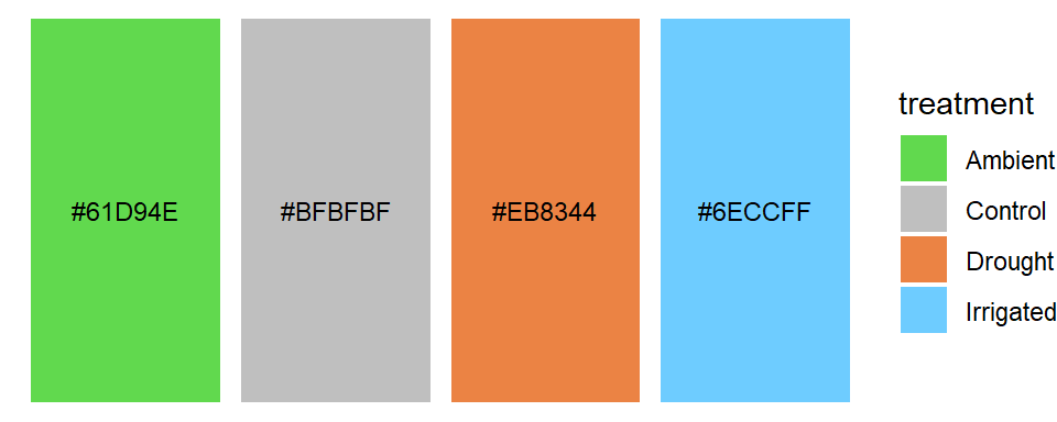

1. Above-ground biomass

Click here to expand

Data summary

Here, cuttings of 1m x 0.25m strips (from ~1cm above the ground) from each treatment and block are sorted by functional group and after drying at 70 $^\circ$ C for over 48 hours their dry mass is weighed in grams. Measurements occur twice per year- one harvest in June in the middle of the growing season and one and in September at the end of the growing season.

Here a summary of the data:

glimpse(biomass)

Rows: 1,199
Columns: 6
$ year      <dbl> 2016, 2016, 2016, 2016, 2016, 2016, 2016, 2016, 2016, 2016, ~
$ harvest   <chr> "Mid", "Mid", "Mid", "Mid", "Mid", "Mid", "Mid", "Mid", "Mid~
$ block     <chr> "A", "A", "A", "A", "A", "A", "A", "A", "A", "A", "A", "A", ~
$ treatment <chr> "Ambient", "Ambient", "Ambient", "Ambient", "Ambient", "Ambi~
$ group     <chr> "Bryophytes", "Dead", "Forbs", "Graminoids", "Legumes", "Woo~
$ biomass_g <dbl> 0.7, 4.5, 16.5, 49.7, 7.7, 0.0, 0.3, 2.4, 20.0, 46.7, 3.6, 1~

$year - year of measurement (integer 2016-2020)
$harvest - point of the growing season when harvest occur (category “Mid” and “End”)
$block - block of experiment (category A-E)
$treatment - experimental treatment for Drought-Net (category “Ambient”, “Control”, “Drought” and “Irrigated”)
$group - functional group of measurement (category “Bryophytes”, “Dead”, “Forbs”, “Graminoids”, “Legumes” and “Woody”)
$biomass_g - above-ground dry mass in grams (continuous)

Biomass variable

Let us first have a look at the response variable biomass_g. We’ll remove any zero observations of biomass. If we plot out the frequency histogram of the raw data, we can see there is some strong positive skew in this variable, because of the differences in biomass scale between our functional groups (i.e. grasses very over-represented).

biomass <- biomass %>% 
  filter(biomass_g > 0)

ggplot(biomass, aes(x = biomass_g)) +
  geom_histogram(bins = 20) +
  labs(x = "Above-ground biomass (g)", y = "Frequency") +
  theme_bw(base_size = 14) +
  theme(panel.grid = element_blank())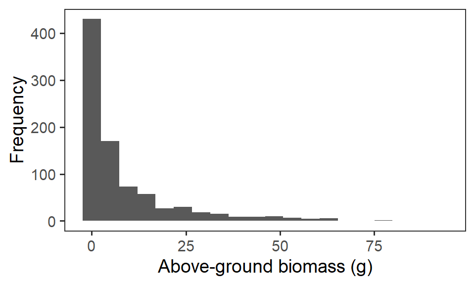

So, instead, for statistical analysis and visualisation, we take the natural logarithm $\ln$ of the raw biomass value.

biomass <- biomass %>% 
  mutate(biomass_log = log(biomass_g))

ggplot(biomass, aes(x = biomass_log)) +
  geom_histogram(bins = 20) +
  labs(x = expression(paste(ln," Above-ground biomass")), y = "Frequency") +
  theme_bw(base_size = 14) +
  theme(panel.grid = element_blank())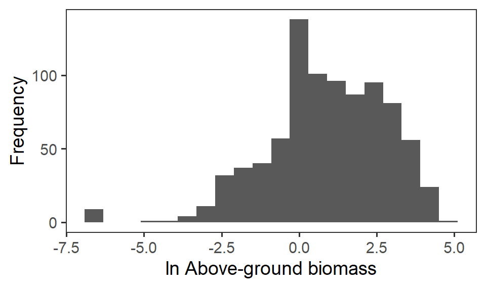

Using the ln biomass variable, we can explore patterns relating to our drought treatments, functional groups, temporal patterns and any potential block effects.

Total biomass

The first interesting question to explore is how biomass overall, which indicates primary productivity, is affected by the rainfall treatments. Here we need to sum up the biomass across functional groups. We again look at the $\ln$ total biomass too. We present here the density plots (violins) with median (total biomass) and mean ( $\ln$ total biomass) points (large holes) as well as underlying raw data (small points).

totbiomass <- biomass %>% 
  group_by(year, harvest, block, treatment) %>% 
  summarise(tot_biomass = sum(biomass_g),
            log_tot_biomass = log(tot_biomass)) %>% 
  ungroup()

And now we can look at how this is affected by the rainfall treatments.

tb_1 <- totbiomass %>% 
  ggplot(aes(x = treatment, y = tot_biomass, 
             fill = treatment)) +
  geom_violin() +
  stat_summary(fun = median, geom = "point", 
               size = 6, shape = 21, fill = "white") +
  geom_jitter(width = 0.1, alpha = 0.4, size = 1)+
  scale_fill_manual(values = raindrop_colours$colour,
                    guide = F) +
  labs(x = "Rainfall treatment", y = "Total above-ground biomass (g)") +
  theme_bw(base_size = 14) +
  theme(panel.grid = element_blank())

tb_2 <- totbiomass %>% 
  ggplot(aes(x = treatment, y = log_tot_biomass, 
             fill = treatment)) +
  geom_violin() +
  stat_summary(fun = mean, geom = "point", 
               size = 6, shape = 21, fill = "white") +
  geom_jitter(width = 0.1, alpha = 0.4, size = 1)+
  scale_fill_manual(values = raindrop_colours$colour,
                    guide = F) +
  labs(x = "Rainfall treatment", 
       y = expression(paste(ln, " Total above-ground biomass"))) +
  theme_bw(base_size = 14) +
  theme(panel.grid = element_blank())

tb_1 + tb_2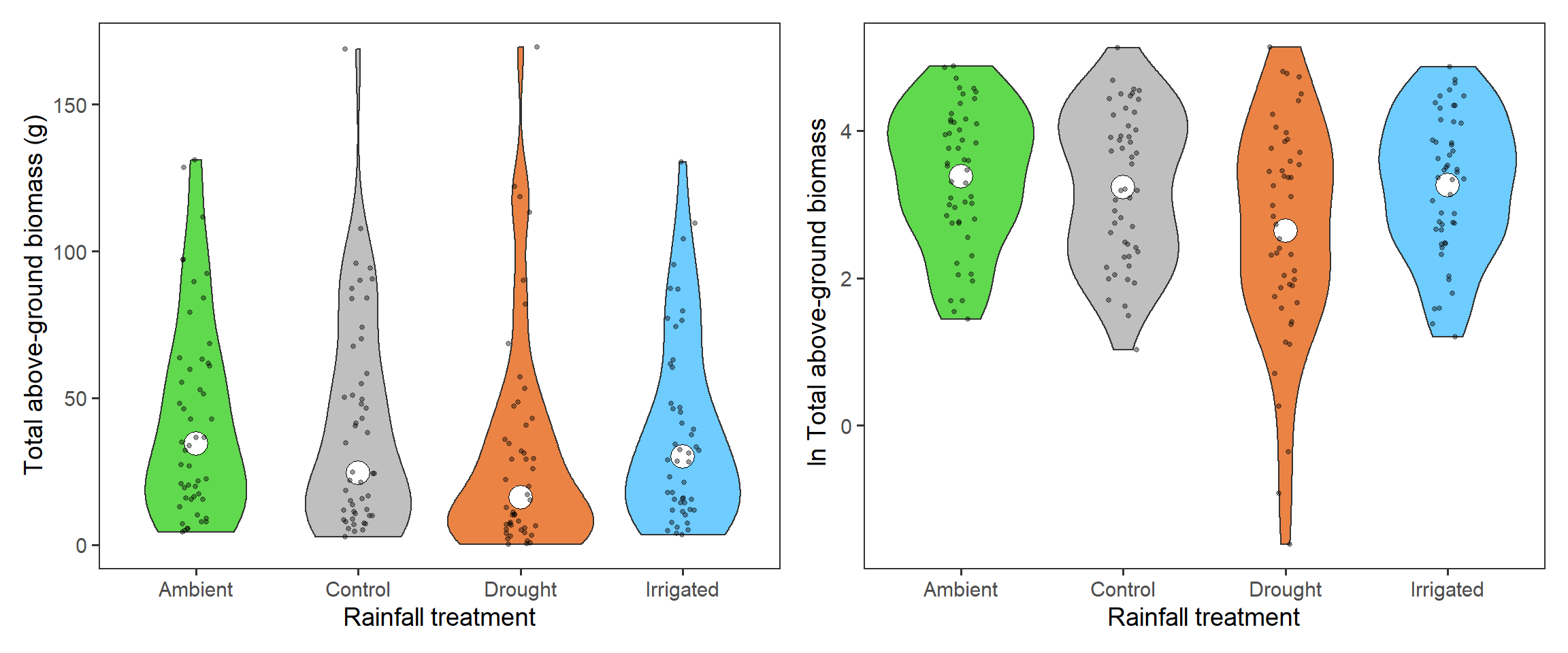

Across all functional groups, years and blocks, it looks like there is a reduction in total biomass associated with the drought treatment.

Now we’ll look at potential temporal effects i.e. whether there is a change in total biomass over time. We first have to add in temporal information to the year and harvest columns, and then we can plot out the total biomass.

# adding temporal information
totbiomass <- totbiomass %>% 
  mutate(month = if_else(harvest == "End", 9, 6),
         date = as.Date(paste0(year,"-",month,"-15")),
         harvest = factor(harvest, levels = c("Mid", "End")))

# plots
totbiomass %>% 
  ggplot(aes(x = date, y = log_tot_biomass, colour = treatment, 
             group = treatment, shape = harvest)) +
  stat_summary(geom = "line", fun = mean, size = 1) +
  stat_summary(geom = "point", fun = mean, size = 3) +
  scale_colour_manual(values = raindrop_colours$colour) +
  labs(x = "Year", y = expression(paste("Mean ", ln, " total biomass")),
       colour = "Treatment", shape = "Harvest") +
  theme_bw(base_size = 14) +
  theme(panel.grid = element_blank())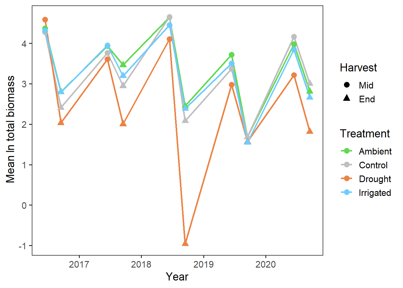

And also splitting out the harvests

totbiomass %>% 
  ggplot(aes(x = year, y = log_tot_biomass, colour = treatment, 
             group = treatment)) +
  stat_summary(geom = "line", fun = mean, size = 1) +
  stat_summary(geom = "point", fun = mean, size = 3) +
  scale_colour_manual(values = raindrop_colours$colour) +
  labs(x = "Year", y = expression(paste("Mean ", ln, " total biomass")),
       colour = "Treatment") +
  facet_wrap(~harvest) +
  theme_bw(base_size = 14) +
  theme(panel.grid = element_blank(),
        strip.background = element_blank())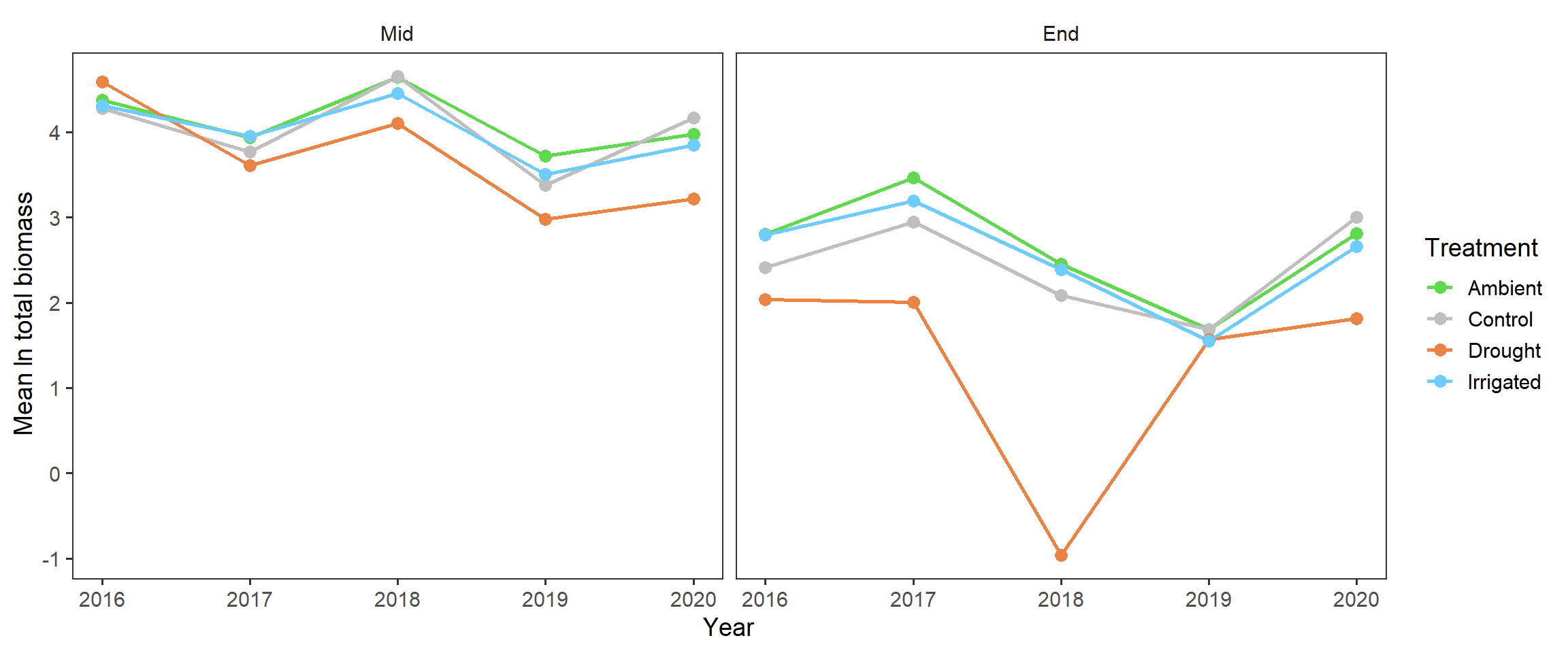

2. Species diversity