Solutions to Exercises
Julien Wollbrett
Swiss Institut of Bioinformatics (SIB), Université de Lausannebgee[at]sib.swiss
2020-04-22
Last updated: 2020-04-28
Checks: 7 0
Knit directory: BgeeCall_practical/
This reproducible R Markdown analysis was created with workflowr (version 1.6.1). The Checks tab describes the reproducibility checks that were applied when the results were created. The Past versions tab lists the development history.
Great! Since the R Markdown file has been committed to the Git repository, you know the exact version of the code that produced these results.
Great job! The global environment was empty. Objects defined in the global environment can affect the analysis in your R Markdown file in unknown ways. For reproduciblity it’s best to always run the code in an empty environment.
The command set.seed(20200421) was run prior to running the code in the R Markdown file. Setting a seed ensures that any results that rely on randomness, e.g. subsampling or permutations, are reproducible.
Great job! Recording the operating system, R version, and package versions is critical for reproducibility.
Nice! There were no cached chunks for this analysis, so you can be confident that you successfully produced the results during this run.
Great job! Using relative paths to the files within your workflowr project makes it easier to run your code on other machines.
Great! You are using Git for version control. Tracking code development and connecting the code version to the results is critical for reproducibility.
The results in this page were generated with repository version 3bcbb2e. See the Past versions tab to see a history of the changes made to the R Markdown and HTML files.
Note that you need to be careful to ensure that all relevant files for the analysis have been committed to Git prior to generating the results (you can use wflow_publish or wflow_git_commit). workflowr only checks the R Markdown file, but you know if there are other scripts or data files that it depends on. Below is the status of the Git repository when the results were generated:
Ignored files:
    Ignored:    .Rhistory
    Ignored:    .Rproj.user/

Untracked files:
    Untracked:  PCA_dim_1vs2.png
    Untracked:  PCA_prop_explained_variance.png
    Untracked:  analyis.R
    Untracked:  dif_expressed_genes.tsv
    Untracked:  inputFile.tsv
    Untracked:  input_files/
    Untracked:  merge.R
    Untracked:  output_files/
    Untracked:  release.tsv

Unstaged changes:
    Deleted:    analysis/exercices.Rmd
Note that any generated files, e.g. HTML, png, CSS, etc., are not included in this status report because it is ok for generated content to have uncommitted changes.
These are the previous versions of the repository in which changes were made to the R Markdown (analysis/solutions.Rmd) and HTML (docs/solutions.html) files. If you’ve configured a remote Git repository (see ?wflow_git_remote), click on the hyperlinks in the table below to view the files as they were in that past version.
| File | Version | Author | Date | Message |
|---|---|---|---|---|
| Rmd | 3bcbb2e | Julien | 2020-04-28 | wflow_publish(files = c(“analysis/analysis.Rmd”, “analysis/classes_description.Rmd”, |
| html | dc40200 | Julien | 2020-04-28 | Build site. |
| Rmd | 4287dd8 | Julien | 2020-04-28 | wflow_publish(files = c(“analysis/analysis.Rmd”, “analysis/classes_description.Rmd”, |
Exercise 1:
R commands to run are :
library(BgeeCall)
# initialize kallisto object
kallisto <- new("KallistoMetadata", download_kallisto = TRUE)
#initialize userr object
user <- new("UserMetadata", species_id = "7227", reads_size=76)
user <- setRNASeqLibPath(user, "input_files/fastq/SRX109273")
user <- setTranscriptomeFromFile(user, "input_files/ensembl/Drosophila_melanogaster.BDGP6.cdna.all.fa.gz")
user <- setAnnotationFromFile(user, "input_files/ensembl/Drosophila_melanogaster.BDGP6.84.gtf.gz")
user <- setOutputDir(user, "output_files/SRX109273")
user <- setWorkingPath(user, "output_files/")
#run generation of presetn/absent calls
output_files_info <- generate_calls_workflow(abundanceMetadata = kallisto, userMetadata = user)
Querying Bgee to get intergenic release information...Start generation of the file containing both transcriptomic
and intergenic regions.File containing both transcriptomic and intergenic regions has
been created successfully.It is the first time you try to use Kallisto downloaded
from this package. Kallisto has to be downloaded. This version of Kallisto
will only be used inside of this package. It will have no impact on your
potential already installed version of Kallisto.
Downloading kallisto for linux...Kallisto has been succesfully installed.Start generation of kallisto index files.kallisto index files have been succesfully created
for species 7227.Will run kallisto using this command line : output_files//kallisto_linux-v0.45.0/kallisto quant -i output_files//intergenic_0.1/7227/kallisto/transcriptome_Drosophila_melanogaster_BDGP6_cdna_all_fa_gz/transcriptome.idx -o output_files/SRX109273 -t 1 --bias input_files/fastq/SRX109273/SRR384924_1.fastq.gz input_files/fastq/SRX109273/SRR384924_2.fastq.gzGenerate file gene2biotype.tsv.Generate file tx2gene.tsv.Warning in .get_cds_IDX(mcols0$type, mcols0$phase): The "phase" metadata column contains non-NA values for features of type
stop_codon. This information was ignored.'select()' returned 1:1 mapping between keys and columnsNote: importing `abundance.h5` is typically faster than `abundance.tsv`reading in files with read.delim (install 'readr' package for speed up)1
transcripts missing from tx2gene: 9
summarizing abundance
summarizing counts
summarizing length
Note: importing `abundance.h5` is typically faster than `abundance.tsv`
reading in files with read.delim (install 'readr' package for speed up)
1
summarizing abundance
summarizing counts
summarizing length
Generate present/absent expression calls.
TPM cutoff for which 95% of the expressed genes are coding found at TPM = 0.716792Answer to questions :
- TPM threshold : 0.716792 (information available in file output_files/SRX109273/gene_cutoff_info_file.tsv)
- Proportion of protein coding present : 69.13 (information available in file output_files/SRX109273/gene_cutoff_info_file.tsv)
- density plot : output_files/SRX109273/gene_TPM_genic_intergenic+cutoff.pdf
Calls of presence/absence are in the file : output_files/SRX109273/gene_level_abundance+calls.tsv
Exercise 2
You have to modify the file inputFile.tsv in order to generate calls on 2 libraries. After modification the file should looks like that :
input_file <- "input_files/inputFile.tsv"
input_file
[1] "input_files/inputFile.tsv"R commands to generate the calls using a file as input :
generate_calls_workflow(abundanceMetadata = kallisto, userFile = "input_files/inputFile.tsv")
Querying Bgee to get intergenic release information...kallisto abundance file already exists for library SRX109273. Abundance file will be overwritten.File containing both transcriptomic and intergenic
regions already exists.Index file already exist. No need to create a new one.Will run kallisto using this command line : /tmp/Rtmpw6JJtX/R.INSTALL629962148de5/BgeeCall/kallisto_linux-v0.45.0/kallisto quant -i /tmp/Rtmpw6JJtX/R.INSTALL629962148de5/BgeeCall/intergenic_0.1/7227/kallisto/transcriptome_Drosophila_melanogaster_BDGP6_cdna_all_fa_gz/transcriptome.idx -o output_files/SRX109273/ -t 1 --bias input_files/fastq/SRX109273//SRR384924_1.fastq.gz input_files/fastq/SRX109273//SRR384924_2.fastq.gzNote: importing `abundance.h5` is typically faster than `abundance.tsv`reading in files with read.delim (install 'readr' package for speed up)1
transcripts missing from tx2gene: 9
summarizing abundance
summarizing counts
summarizing length
Note: importing `abundance.h5` is typically faster than `abundance.tsv`
reading in files with read.delim (install 'readr' package for speed up)
1
summarizing abundance
summarizing counts
summarizing length
Generate present/absent expression calls.
TPM cutoff for which 95% of the expressed genes are coding found at TPM = 0.716792
File containing both transcriptomic and intergenic
                regions already exists.
Index file already exist. No need to create a new one.
Will run kallisto using this command line : /tmp/Rtmpw6JJtX/R.INSTALL629962148de5/BgeeCall/kallisto_linux-v0.45.0/kallisto quant -i /tmp/Rtmpw6JJtX/R.INSTALL629962148de5/BgeeCall/intergenic_0.1/7227/kallisto/transcriptome_Drosophila_melanogaster_BDGP6_cdna_all_fa_gz/transcriptome.idx -o output_files/SRX109272/ -t 1 --bias input_files/fastq/SRX109272//SRR384923_1.fastq.gz input_files/fastq/SRX109272//SRR384923_2.fastq.gz
Note: importing `abundance.h5` is typically faster than `abundance.tsv`
reading in files with read.delim (install 'readr' package for speed up)
1
transcripts missing from tx2gene: 9
summarizing abundance
summarizing counts
summarizing length
Note: importing `abundance.h5` is typically faster than `abundance.tsv`
reading in files with read.delim (install 'readr' package for speed up)
1
summarizing abundance
summarizing counts
summarizing length
Generate present/absent expression calls.
TPM cutoff for which 95% of the expressed genes are coding found at TPM = 0.379585NULLAnswer to questions :
- TPM threshold : 0.379585 (information available in file output_files/SRX109272/gene_cutoff_info_file.tsv)
- Proportion of protein coding present : 67.39 (information available in file output_files/SRX109272/gene_cutoff_info_file.tsv)
- density plot : output_files/SRX109272/gene_TPM_genic_intergenic+cutoff.pdf
- calls are in the file output_files/SRX109272/gene_level_abundance+calls.tsv
calls_SRX109272 <- read.table("output_files/SRX109272/gene_level_abundance+calls.tsv", header = TRUE, sep = "\t")
head(calls_SRX109272)
id abundance counts length biotype type call
1 FBgn0000008 16.4878960 297.000150 4626.628 protein_coding genic present
2 FBgn0000014 0.2690010 4.000000 3819.270 protein_coding genic absent
3 FBgn0000015 0.1107308 1.999998 4639.135 protein_coding genic absent
4 FBgn0000017 22.2918200 561.994850 6475.303 protein_coding genic present
5 FBgn0000018 0.6565900 4.000000 1564.730 protein_coding genic present
6 FBgn0000022 0.0000000 0.000000 784.193 protein_coding genic absentExercise 3
R commands to generate the PCA plots :
# read file with gene as rows and libraries as columns
file <- "input_files/downstream_analysis/present_TPMs.tsv"
present_TPMs <- read.table(file = file, header = TRUE, sep = "\t")
# transpose data.frame to have genes as columns
data_for_PCA <- t(present_TPMs)
# calculate matrix of dissimilarities
# k = the maximum dimension of the space which the data are to be represented in; must be in {1, 2, …, n-1}
# eig = indicates whether eigenvalues should be returned
mds <- cmdscale(dist(data_for_PCA), k=3, eig=TRUE)
proportion_eig <- mds$eig * 100 / sum(mds$eig)
# plot proportion of variance explained by each dimension
barplot(proportion_eig, las=1, ylim=c(0,100), xlab="Dimensions", ylab="Proportion of explained variance (%)",
        y.axis=NULL, col="darkgrey", main = "Proportion of variance explained by each dimension")
| Version | Author | Date |
|---|---|---|
| dc40200 | Julien | 2020-04-28 |
#PCA plot for the 2 first dimensions
#plotMDS(present_TPMs,xlab = "Dimension 1")
plot(mds$points[,1], -mds$points[,2], type="n", xlim=c(-2.5e+05,2.5e+05), xlab="Dimension 1", ylab="Dimension 2",
     main="PCA plot of the 2 principal dimensions", )
text(mds$points[,1], -mds$points[,2], rownames(mds$points), cex=0.8)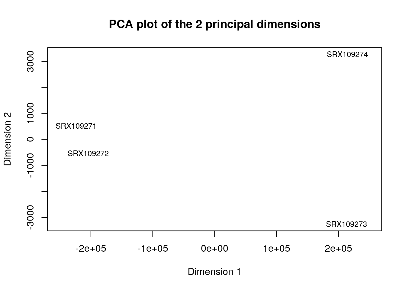
| Version | Author | Date |
|---|---|---|
| dc40200 | Julien | 2020-04-28 |
Answer to questions :
* Libraries SRX109273 and SRX109274 cluster together. Libraries SRX109271 and SRX109272 cluster together * Looking at library annotations we can see that all libraries correspond to same anatomical entity, developmental stage and strain. The only difference is the sex. In the plot we see that one dimension explains all variance between libraries. It means one biological parameter explains all the variance. This parameter is the sex as female samples cluster together and male samples cluster together. In the next Exercise we will calculate differential expression of male samples versus female samples.
Exercise 4 :
R commands to generate the differential expression (DE) :
library(edgeR)Loading required package: limma# read file with gene as rows and libraries counts as columns
file_counts <- "input_files/downstream_analysis/present_counts.tsv"
present_counts <- read.table(file = file_counts, header = TRUE, sep = "\t")
#read file with library annotations
file_annotations <- "input_files/downstream_analysis/library_annotations.tsv"
library_annotations <- read.table(file = file_annotations, header = TRUE, sep = "\t")
# create list of grouping parameters (here sex)
group <- NULL
for(i in seq(colnames(present_counts))){
group[i] <- as.character(library_annotations[library_annotations$Library.ID ==colnames(present_counts)[i],]$Sex)
}
# create DGEList object
dge <- DGEList(present_counts, group=group)
#calculate normalization factor between libraries
dge <- calcNormFactors(dge)
#estimate common and tag wise dispersion
dge <- estimateCommonDisp(dge)
dge <- estimateTagwiseDisp(dge)
#perform an exact test for the difference in expression male-female
dgeTest <- exactTest(dge)
# retrieve all gene differentially expressed with a p-value lower than 0.05
topTags <- topTags(dgeTest, n=nrow(dgeTest$table), p.value = 0.01)
#filter for FDR < 0.05
results <- topTags$table[topTags$table$FDR<0.05,]
#number of genes DE with pvalue<0.05 and fdr<0.05
nrow(results)[1] 1929write.table(x = results, file = "dif_expressed_genes.tsv", row.names = TRUE, quote = FALSE, sep="\t")
# generate an MA plot with 1% differentially expressed genes
plotSmear(dgeTest, de.tags = rownames(topTags$table)[which(topTags$table$FDR<0.01)],)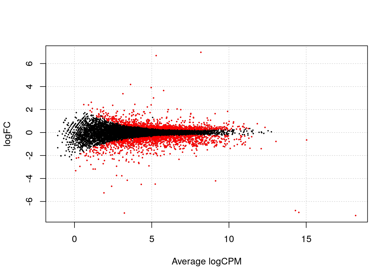
| Version | Author | Date |
|---|---|---|
| dc40200 | Julien | 2020-04-28 |
# generate a volcano plot
volcanoData <- cbind(topTags$table$logFC, -log10(topTags$table$PValue))
colnames(volcanoData) <- c("logFC", "negLogPval")
plot(volcanoData, pch=19)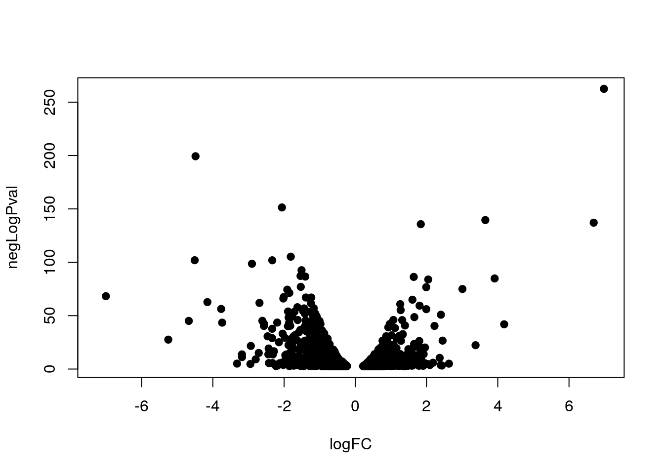
| Version | Author | Date |
|---|---|---|
| dc40200 | Julien | 2020-04-28 |
Answer to questions :
* top ten most DE genes (ordered by logFC for pvalue<0.05 and FDR<0.05):
head(x = results,n = 10) logFC logCPM PValue FDR
FBgn0004045 -7.224676 18.199115 0.000000e+00 0.000000e+00
FBgn0005391 -6.952524 14.522168 0.000000e+00 0.000000e+00
FBgn0004047 -6.786418 14.301112 0.000000e+00 0.000000e+00
FBgn0038914 -4.206187 9.133461 0.000000e+00 0.000000e+00
FBgn0036717 6.980602 8.182132 3.392958e-263 6.034714e-260
FBgn0026403 -4.486764 5.228902 4.879407e-200 7.232094e-197
FBgn0030041 -2.060106 7.876724 4.423706e-152 5.620003e-149
FBgn0038074 3.650463 5.769394 2.790223e-140 3.101681e-137
FBgn0039685 6.693557 5.288792 8.328659e-138 8.229641e-135
FBgn0002565 1.838322 9.910885 2.020245e-136 1.796604e-133- number of DE genes for pvalue<0.01 and logFC>2
#add cutoff for logFC and pvalue
results_filter <- results[abs(results$logFC)>2 & results$PValue<0.01,]
#number of DE genes with new filters :
nrow(results_filter)
[1] 64- run again DE analysis with both present/absent calls.
file_counts_all <- "input_files/downstream_analysis/all_counts.tsv"
all_counts <- read.table(file = file_counts_all, header = TRUE, sep = "\t")
dge_all <- DGEList(all_counts, group=group)
dge_all <- calcNormFactors(dge_all)
dge_all <- estimateCommonDisp(dge_all)
dge_all <- estimateTagwiseDisp(dge_all)
dgeTest_all <- exactTest(dge_all)
topTags_all <- topTags(dgeTest_all, n=nrow(dgeTest_all$table), p.value = 0.05)
results_all <- topTags_all$table[topTags_all$table$FDR<0.05,]
#number of DE genes detected
nrow(results_all)
[1] 2633#add cutoff for logFC and pvalue
results_all_filter <- results_all[abs(results_all$logFC)>2 & results_all$PValue<0.01,]
nrow(results_all_filter)[1] 244Optional Exercise
Example of R code to run a GO analysis :
library(biomaRt)
## topGO function of edgeR require entrez IDs. We will use biomaRt to map ensembl Ids to entrez Ids
#query biomaRt
mart <- useDataset("dmelanogaster_gene_ensembl", useMart("ensembl"))
entrez_mapping <- getBM(attributes=c("ensembl_gene_id", "entrezgene_id"), mart=mart, useCache = FALSE)
#update row names of the DGEExact object from edgeR
table <- merge(dgeTest$table, entrez_mapping, by.x="row.names", by.y="ensembl_gene_id", all.x = TRUE)
#looks like mapping from biomaRt has some problems of redundancy. Need hack to remove redundancy (not good practice)
table <- na.omit(table[!duplicated(table[,c('entrezgene_id')]),])
rownames(table) <- table$entrezgene_id
dgeTest$table <- table[,c('logFC','logCPM','PValue')]

#run the GO analysis
go <- goana(dgeTest, species = "Dm")
topGO(go)
Term Ont N Up Down P.Up
GO:0022626 cytosolic ribosome CC 91 0 86 1.0000000
GO:0002181 cytoplasmic translation BP 117 0 94 1.0000000
GO:0042254 ribosome biogenesis BP 191 3 123 1.0000000
GO:0022613 ribonucleoprotein complex biogenesis BP 268 6 138 1.0000000
GO:0044445 cytosolic part CC 143 6 93 0.9999738
GO:0022625 cytosolic large ribosomal subunit CC 52 0 51 1.0000000
GO:0006364 rRNA processing BP 124 3 80 0.9999985
GO:0005840 ribosome CC 174 4 96 1.0000000
GO:0016072 rRNA metabolic process BP 142 4 85 0.9999990
GO:0044391 ribosomal subunit CC 165 3 92 1.0000000
GO:0006412 translation BP 367 9 151 1.0000000
GO:0043604 amide biosynthetic process BP 425 16 166 1.0000000
GO:0043043 peptide biosynthetic process BP 401 12 159 1.0000000
GO:1990904 ribonucleoprotein complex CC 556 26 197 1.0000000
GO:0005730 nucleolus CC 185 6 95 0.9999999
GO:0043603 cellular amide metabolic process BP 526 30 186 1.0000000
GO:0003735 structural constituent of ribosome MF 158 4 86 0.9999999
GO:0006518 peptide metabolic process BP 464 23 168 1.0000000
GO:0042273 ribosomal large subunit biogenesis BP 51 0 43 1.0000000
GO:0022627 cytosolic small ribosomal subunit CC 38 0 36 1.0000000
P.Down
GO:0022626 1.966044e-62
GO:0002181 9.423063e-54
GO:0042254 4.884838e-52
GO:0022613 3.330418e-42
GO:0044445 5.653007e-40
GO:0022625 9.007390e-40
GO:0006364 4.019224e-34
GO:0005840 1.061884e-32
GO:0016072 1.223935e-32
GO:0044391 7.403915e-32
GO:0006412 1.165862e-31
GO:0043604 1.531185e-31
GO:0043043 4.264480e-31
GO:1990904 1.069313e-30
GO:0005730 4.486529e-29
GO:0043603 7.974862e-29
GO:0003735 8.356819e-29
GO:0006518 2.293887e-27
GO:0042273 9.169436e-27
GO:0022627 1.126329e-26
sessionInfo()R version 3.6.3 (2020-02-29)
Platform: x86_64-pc-linux-gnu (64-bit)
Running under: Ubuntu 18.04.4 LTS
Matrix products: default
BLAS: /usr/lib/x86_64-linux-gnu/openblas/libblas.so.3
LAPACK: /usr/lib/x86_64-linux-gnu/libopenblasp-r0.2.20.so
locale:
[1] LC_CTYPE=en_GB.UTF-8 LC_NUMERIC=C
[3] LC_TIME=fr_FR.UTF-8 LC_COLLATE=en_GB.UTF-8
[5] LC_MONETARY=fr_FR.UTF-8 LC_MESSAGES=en_GB.UTF-8
[7] LC_PAPER=fr_FR.UTF-8 LC_NAME=C
[9] LC_ADDRESS=C LC_TELEPHONE=C
[11] LC_MEASUREMENT=fr_FR.UTF-8 LC_IDENTIFICATION=C
attached base packages:
[1] stats graphics grDevices utils datasets methods base
other attached packages:
[1] biomaRt_2.42.0 edgeR_3.28.1 limma_3.42.2 BgeeCall_1.2.1
[5] workflowr_1.6.1
loaded via a namespace (and not attached):
[1] Biobase_2.46.0 httr_1.4.1
[3] bit64_0.9-7 jsonlite_1.6.1
[5] assertthat_0.2.1 askpass_1.1
[7] stats4_3.6.3 BiocFileCache_1.10.2
[9] blob_1.2.1 GenomeInfoDbData_1.2.2
[11] Rsamtools_2.2.3 yaml_2.2.1
[13] progress_1.2.2 pillar_1.4.3
[15] RSQLite_2.2.0 backports_1.1.5
[17] lattice_0.20-41 glue_1.3.1
[19] digest_0.6.25 GenomicRanges_1.38.0
[21] promises_1.1.0 XVector_0.26.0
[23] htmltools_0.4.0 httpuv_1.5.2
[25] Matrix_1.2-18 XML_3.99-0.3
[27] pkgconfig_2.0.3 zlibbioc_1.32.0
[29] GO.db_3.10.0 purrr_0.3.3
[31] whisker_0.4 org.Dm.eg.db_3.10.0
[33] later_1.0.0 BiocParallel_1.20.1
[35] git2r_0.26.1 tibble_2.1.3
[37] openssl_1.4.1 IRanges_2.20.2
[39] SummarizedExperiment_1.16.1 GenomicFeatures_1.38.2
[41] BiocGenerics_0.32.0 magrittr_1.5
[43] crayon_1.3.4 memoise_1.1.0
[45] evaluate_0.14 fs_1.3.2
[47] tools_3.6.3 prettyunits_1.1.1
[49] hms_0.5.3 matrixStats_0.55.0
[51] stringr_1.4.0 Rhdf5lib_1.8.0
[53] S4Vectors_0.24.3 locfit_1.5-9.4
[55] DelayedArray_0.12.2 AnnotationDbi_1.48.0
[57] Biostrings_2.54.0 compiler_3.6.3
[59] GenomeInfoDb_1.22.0 rlang_0.4.5
[61] rhdf5_2.30.1 grid_3.6.3
[63] RCurl_1.98-1.1 tximport_1.14.0
[65] rappdirs_0.3.1 bitops_1.0-6
[67] rmarkdown_2.1 DBI_1.1.0
[69] curl_4.3 R6_2.4.1
[71] GenomicAlignments_1.22.1 knitr_1.28
[73] dplyr_0.8.4 rtracklayer_1.46.0
[75] bit_1.1-15.2 rprojroot_1.3-2
[77] stringi_1.4.6 parallel_3.6.3
[79] Rcpp_1.0.3 vctrs_0.2.3
[81] dbplyr_1.4.2 tidyselect_1.0.0
[83] xfun_0.12