Last updated: 2024-11-01

Checks: 7 0

Knit directory: 2021_MPSIIIBvQ96-RNAseq-7dpfLarve/

This reproducible R Markdown analysis was created with workflowr (version 1.7.1). The Checks tab describes the reproducibility checks that were applied when the results were created. The Past versions tab lists the development history.

R Markdown file: up-to-date

Great! Since the R Markdown file has been committed to the Git repository, you know the exact version of the code that produced these results.

Environment: empty

Great job! The global environment was empty. Objects defined in the global environment can affect the analysis in your R Markdown file in unknown ways. For reproduciblity it’s best to always run the code in an empty environment.

Seed: set.seed(20211120)

The command set.seed(20211120) was run prior to running the code in the R Markdown file. Setting a seed ensures that any results that rely on randomness, e.g. subsampling or permutations, are reproducible.

Session information: recorded

Great job! Recording the operating system, R version, and package versions is critical for reproducibility.

Cache: none

Nice! There were no cached chunks for this analysis, so you can be confident that you successfully produced the results during this run.

File paths: relative

Great job! Using relative paths to the files within your workflowr project makes it easier to run your code on other machines.

Repository version: 7bb9ce6

Great! You are using Git for version control. Tracking code development and connecting the code version to the results is critical for reproducibility.

The results in this page were generated with repository version 7bb9ce6. See the Past versions tab to see a history of the changes made to the R Markdown and HTML files.

Note that you need to be careful to ensure that all relevant files for the analysis have been committed to Git prior to generating the results (you can use wflow_publish or wflow_git_commit). workflowr only checks the R Markdown file, but you know if there are other scripts or data files that it depends on. Below is the status of the Git repository when the results were generated:


Ignored files:
    Ignored:    .DS_Store
    Ignored:    .RData
    Ignored:    .Rapp.history
    Ignored:    .Rhistory
    Ignored:    .Rproj.user/
    Ignored:    analysis/.DS_Store
    Ignored:    code/.DS_Store
    Ignored:    code/6mBrain_RNAseq_genoSex.rmd
    Ignored:    code/6mBrain_fems.rmd
    Ignored:    code/HS.R
    Ignored:    code/about.Rmd
    Ignored:    code/analysis.Rmd
    Ignored:    code/analysis_final.rmd
    Ignored:    code/analysis_final_v2.rmd
    Ignored:    code/checkGenotypes.rmd
    Ignored:    code/explorationRUV.Rmd
    Ignored:    code/genotypeCheck.Rmd
    Ignored:    code/license.Rmd
    Ignored:    code/nhi6mdata.rmd
    Ignored:    code/plots4pub2.rmd
    Ignored:    code/plots4pub_RNAseq_afterreview1.R
    Ignored:    code/wgcna.rmd
    Ignored:    data/.DS_Store
    Ignored:    data/Nhi_data/.DS_Store
    Ignored:    data/R_objects/.DS_Store
    Ignored:    data/R_objects/larvae/.DS_Store
    Ignored:    data/adult_brain/.DS_Store
    Ignored:    data/adult_brain/05_featureCounts/.DS_Store
    Ignored:    data/adult_brain/fastqc_raw/.DS_Store
    Ignored:    data/gene_sets/.DS_Store
    Ignored:    data/larvae/.DS_Store
    Ignored:    data/larvae/fastqc_align/.DS_Store
    Ignored:    data/larvae/fastqc_align_dedup/.DS_Store
    Ignored:    data/larvae/fastqc_raw/.DS_Store
    Ignored:    data/larvae/fastqc_trim/.DS_Store
    Ignored:    data/larvae/featureCounts/.DS_Store
    Ignored:    data/larvae/meta/.DS_Store
    Ignored:    data/larvae/starAlignLog/.DS_Store
    Ignored:    output/.DS_Store
    Ignored:    output/plots/
    Ignored:    output/plots4poster/.DS_Store
    Ignored:    output/plots4pub/

Untracked files:
    Untracked:  Rplot01.pdf
    Untracked:  Rplot02.png
    Untracked:  data/R_objects/adult_brain/HMPKEGG_6m_brain_genosex_CQN.rds
    Untracked:  data/R_objects/adult_brain/HMP_ire_6m_brain_genosex_CQN.rds
    Untracked:  data/R_objects/adult_brain/cqn_logCPM_6m_brain.rds
    Untracked:  data/R_objects/adult_brain/dge_6m_brain_cqn.rds
    Untracked:  data/R_objects/adult_brain/fry_cell_6m_brain_genosex_CQN.rds
    Untracked:  data/R_objects/adult_brain/fry_cell_RNAseq.rds
    Untracked:  data/R_objects/adult_brain/goseqtibbles_6m_brain_genosex_CQN.rds
    Untracked:  data/R_objects/adult_brain/hmp.kegg.rna.rds
    Untracked:  data/R_objects/adult_brain/toptablescqn_bysex.rds
    Untracked:  data/allLLIDs.rds
    Untracked:  data/ensembl_zebrafish.rds
    Untracked:  data/proteomics/
    Untracked:  data/with_go_evidence.rds
    Untracked:  dre00020.pathview.multi.png
    Untracked:  dre00020.png
    Untracked:  dre00020.xml
    Untracked:  hsa04650.EOfADproteomes.multi.png
    Untracked:  hsa04650.MPSIIIBproteomes.multi.png
    Untracked:  hsa04650.png
    Untracked:  hsa04650.xml
    Untracked:  hsa04666.EOfADproteomes.multi.png
    Untracked:  hsa04666.MPSIIIBproteomes.multi.png
    Untracked:  hsa04666.png
    Untracked:  hsa04666.xml
    Untracked:  larvae dre00020.pathview.multi.png
    Untracked:  output/DE_proteins_for_string/
    Untracked:  output/GOenrichment_enrichmentTable.csv
    Untracked:  output/plots4RADposter/
    Untracked:  output/plots4kim/
    Untracked:  output/plots4pub2/
    Untracked:  output/plots4pub3/
    Untracked:  output/spreadsheets/RNAseqlarvae_celltypeFry.xlsx
    Untracked:  output/spreadsheets/RNAseqlarvae_hmpoutputs.xlsx
    Untracked:  output/spreadsheets/geneset_RNAseq_v2.xlsx
    Untracked:  output/spreadsheets/goseq_RNAseq_v2.xlsx
    Untracked:  output/spreadsheets/limma_proteomics_6mbrain.xlsx
    Untracked:  output/spreadsheets/proteomics_6mbrain_hmpoutputs.xlsx
    Untracked:  output/spreadsheets/toptables_RNAseq_v2.xlsx
    Untracked:  output/spreadsheets/~$toptables_RNAseq_v2.xlsx
    Untracked:  temp.png

Unstaged changes:
    Modified:   .gitignore
    Deleted:    analysis/6mBrain_fems.rmd
    Deleted:    analysis/HS.R
    Deleted:    analysis/about.Rmd
    Deleted:    analysis/analysis.Rmd
    Deleted:    analysis/analysis_adultbrain.knit.md
    Deleted:    analysis/analysis_final.rmd
    Deleted:    analysis/checkGenotypes.rmd
    Deleted:    analysis/explorationRUV.Rmd
    Deleted:    analysis/genotypeCheck.Rmd
    Deleted:    analysis/license.Rmd
    Deleted:    analysis/nhi6mdata.rmd
    Deleted:    analysis/plots4pub2.rmd
    Modified:   data/R_objects/adult_brain/dge.rds
    Modified:   data/R_objects/adult_brain/hmp_ire.rds
    Modified:   data/R_objects/adult_brain/logcpm.rds
    Modified:   data/R_objects/larvae/celltype_larvae.rds
    Modified:   data/R_objects/larvae/dge.rds
    Modified:   data/R_objects/larvae/hmp_ire.rds
    Modified:   data/R_objects/larvae/hmp_kegg.rds
    Modified:   data/R_objects/larvae/logcpm.rds
    Modified:   data/R_objects/larvae/toptablescqn.rds
    Modified:   data/adult_brain/karissas_metadata.xlsx
    Modified:   output/spreadsheets/toptables_cqn.xlsx

Note that any generated files, e.g. HTML, png, CSS, etc., are not included in this status report because it is ok for generated content to have uncommitted changes.

These are the previous versions of the repository in which changes were made to the R Markdown (analysis/analysis_larvae.Rmd) and HTML (docs/analysis_larvae.html) files. If you’ve configured a remote Git repository (see ?wflow_git_remote), click on the hyperlinks in the table below to view the files as they were in that past version.

File	Version	Author	Date	Message
Rmd	7bb9ce6	Karissa Barthelson	2024-11-01	wflow_publish("analysis/*")

Introduction

library(tidyverse)
library(magrittr)
library(readxl)
library(ngsReports)
library(AnnotationHub)
library(msigdbr)
library(pander)
library(scales)
library(pheatmap)
library(ggpubr)
library(ggrepel)
library(ggfortify)
library(ggforce)
library(RColorBrewer)
library(colorspace)
library(UpSetR)
library(edgeR)
library(goseq)
library(fgsea)

library(cqn)
library(harmonicmeanp)
library(ssizeRNA)
library(variancePartition)

theme_set(theme_bw())

ah <- AnnotationHub() %>%
    subset(species == "Danio rerio") %>%
    subset(rdataclass == "EnsDb")

ensDb <- ah[["AH83189"]] # for release 101, latest version in Ah
grTrans <- transcripts(ensDb)
trLengths <- exonsBy(ensDb, "tx") %>%
    width() %>%
    vapply(sum, integer(1))
mcols(grTrans)$length <- trLengths[names(grTrans)]
gcGene <- grTrans %>%
  mcols() %>%
  as.data.frame() %>%
  dplyr::select(gene_id, tx_id, gc_content, length) %>%
  as_tibble() %>%
  group_by(gene_id) %>%
  summarise(
    gc_content = sum(gc_content*length) / sum(length),
    length = ceiling(median(length))
  )
grGenes <- genes(ensDb)
mcols(grGenes) %<>%
  as.data.frame() %>%
  left_join(gcGene) %>%
  as.data.frame() %>%
  DataFrame()

# read in metadata and cleanup column names and types. 
meta <- read_excel("data/larvae/meta/naglu_v_Q96_larvae_metadata.xlsx", sheet = 3) %>% 
  na.omit() %>% 
  left_join(read_excel("data/larvae/meta/naglu_v_Q96_larvae_metadata.xlsx", sheet = 5) %>% 
              mutate(temp1 = str_split(temp, pattern = " ")) %>% 
              mutate(ULN = lapply(temp1, function(x){
                x %>% 
                  .[1]
              }), 
              sample_name =  lapply(temp1, function(x){
                x %>% 
                  .[2]
              }), 
              RIN = lapply(temp1, function(x){
                x %>% 
                  .[4]
              })
              ) %>% 
              unnest() %>% 
              dplyr::select(ULN, sample_name, RIN) %>% 
              na.omit() %>% 
              unique
  ) %>% 
  mutate(Genotype = case_when(
    `naglu genotype` == "wt" & `psen1 genotype` == "wt" ~ "wt",
    `naglu genotype` == "A603fs/A603fs" & `psen1 genotype` == "wt" ~ "MPSIIIB",
    `naglu genotype` == "wt" & `psen1 genotype` == "Q96_K97del/+" ~ "EOfADlike",
  ) %>% 
    factor(levels = c("wt", "MPSIIIB", "EOfADlike")), 
  sample = paste0(Genotype, "_", ULN), 
  RIN = as.numeric(RIN)) 

# read in the output of featurecounts. 
featureCounts <- 
  read_delim("data/larvae/featureCounts/counts.out", delim = "\t", skip = 1) %>%
  set_names(basename(names(.))) %>% 
  set_names(names(.) %>% str_remove(pattern = "_S1_merged.Aligned.sortedByCoord.dedup.out.bam")) %>% 
  as_tibble() %>% 
  dplyr::select(-c(Chr, Start, End, Length, Strand)) %>% 
  gather(key = "ULN", value = "counts", starts_with("21")) %>% 
  left_join(meta) %>% 
  dplyr::select(Geneid, counts, sample) %>% 
  spread(key = "sample", value = "counts") %>% 
  column_to_rownames("Geneid")

# write out the cleaned up output for uploading to GEO
#write_csv(rownames_to_column(featureCounts, "gene_id"), "output/GEOcounts.out")

filter lowly expressed genes

Genes which are lowly expressed are considered uninformative for de analysis. Here, we set the threshold to be a min CPM of 0.5 (following the 10/min lib size rule proposed by gordon smyth). The effect of filtering is found below

a <- featureCounts %>% 
    cpm(log = TRUE) %>%
    as.data.frame() %>% 
  pivot_longer(
    cols = everything(),
    names_to = "sample",
    values_to = "logCPM"
  ) %>%
  split(f = .$sample) %>%
  lapply(function(x){
    d <- density(x$logCPM)
    tibble(
      sample = unique(x$sample),
      x = d$x,
      y = d$y
    )
  }) %>%
  bind_rows() %>%
  left_join(meta) %>% 
  ggplot(aes(x, y, colour = Genotype, group = sample)) +
  geom_line() +
  labs(
    x = "logCPM",
    y = "Density",
    colour = "Genotype"
  )+
  ggtitle("Before filtering") +
  theme_bw()


b <- featureCounts %>% 
  .[rowSums(cpm(.) >= 0.5) >= 8,] %>% 
    cpm(log = TRUE) %>%
    as.data.frame() %>% 
  pivot_longer(
    cols = everything(),
    names_to = "sample",
    values_to = "logCPM"
  ) %>%
  split(f = .$sample) %>%
  lapply(function(x){
    d <- density(x$logCPM)
    tibble(
      sample = unique(x$sample),
      x = d$x,
      y = d$y
    )
  }) %>%
  bind_rows() %>%
  left_join(meta) %>% 
  ggplot(aes(x, y, colour = Genotype, group = sample)) +
  geom_line() +
  labs(
    x = "logCPM",
    y = "Density",
    colour = "Genotype"
  )+
  ggtitle("After filtering")

ggarrange(a, b, common.legend = TRUE)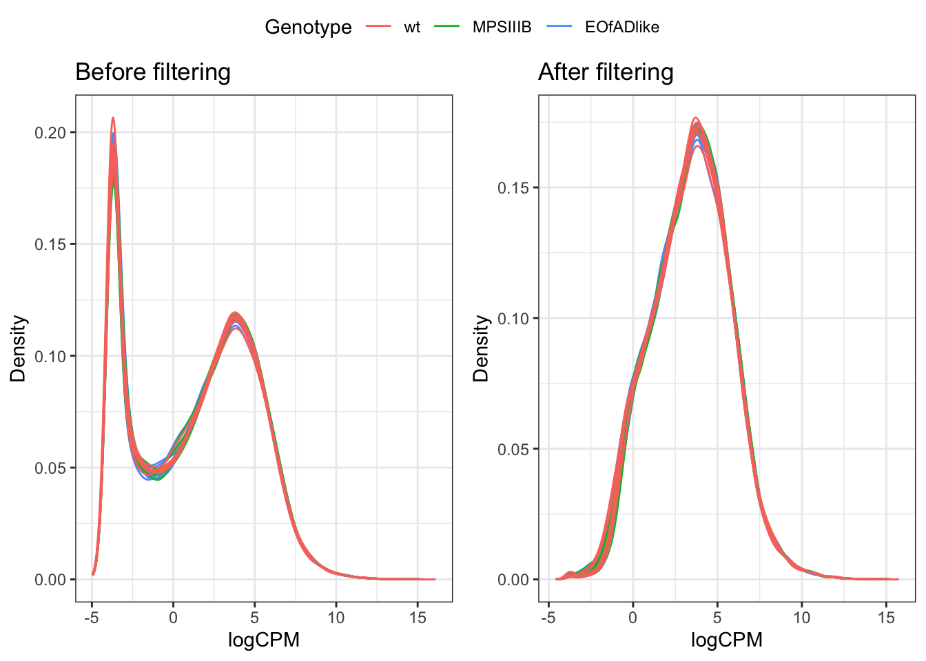

x <- featureCounts %>% 
  as.matrix() %>% 
  .[rowSums(cpm(.) >= 0.5) >= 8,] %>%
  DGEList(
    samples = tibble(sample = colnames(.)) %>%
      left_join(meta),
    genes = grGenes[rownames(.)] %>%
      as.data.frame() %>%
      dplyr::select(
        chromosome = seqnames, start, end, 
        gene_id, gene_name, gene_biotype, description, entrezid
      ) %>% 
      left_join(gcGene) %>% 
      as_tibble()
  ) %>%
  calcNormFactors()

PCA

I fors want to explore the overall similarity between samples by PCA. No distinct clusters of samples are observed by genotype

x$counts %>% 
  cpm(log=TRUE) %>% 
  t() %>% 
  prcomp() %>% 
  autoplot(data = tibble(sample = rownames(.$x)) %>%
      left_join(x$samples),
    colour = "Genotype", 
    size = 6
  ) +
  theme_bw() + 
  theme(aspect.ratio = 1) +
  scale_color_discrete_qualitative(palette = "Dark 3")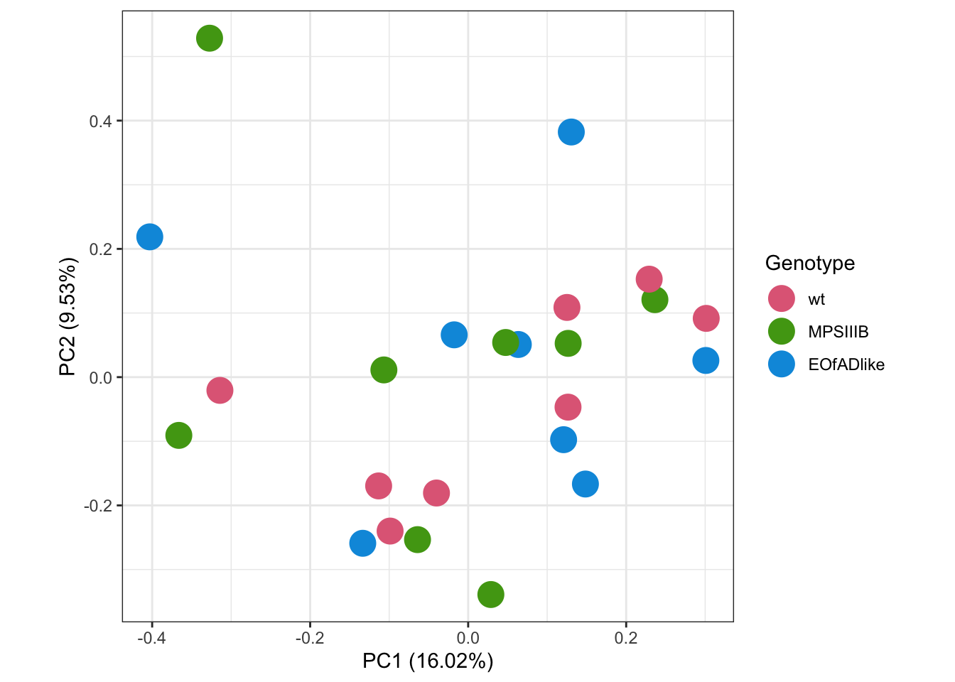

#  ggsave("output/plots/PCAblue.png", width = 10, height = 10, units = "cm", dpi = 300, scale = 1.25)

x$counts %>% 
  cpm(log=TRUE) %>% 
  t() %>% 
  prcomp() %>% 
  autoplot(data = tibble(sample = rownames(.$x)) %>%
      left_join(x$samples),
    colour = "RIN", 
    size = 6
  ) +
  theme_bw() + 
  theme(aspect.ratio = 1) +
  labs(colour = "RIN") +
  scale_color_viridis_c(end = 0.9)

Check genotypes

This is in the checkGenotypes.rmd file. All fish carry the genotypes indicated from the PCR genotyping.

%GC and Length check

design <- model.matrix(~Genotype, data = x$samples) %>% 
  set_colnames(gsub(colnames(.), pattern = "Genotype", replacement = ""))

fit_1 <- x %>% 
  estimateDisp(design) %>% 
  glmFit(design)

# Call the toptable
toptable_1 <- design %>% colnames() %>% .[2:3] %>% 
  sapply(function(x){
    glmLRT(fit_1, coef = x) %>%
      topTags(n = Inf) %>%
      .[["table"]] %>%
      as_tibble() %>%
      arrange(PValue) %>%
       mutate(
        coef = x,
        DE = FDR < 0.05
      ) %>% 
      dplyr::select(
        gene_name, logFC, logCPM, PValue, FDR, DE, everything()  
      )
      
  }, simplify = FALSE)

Vis

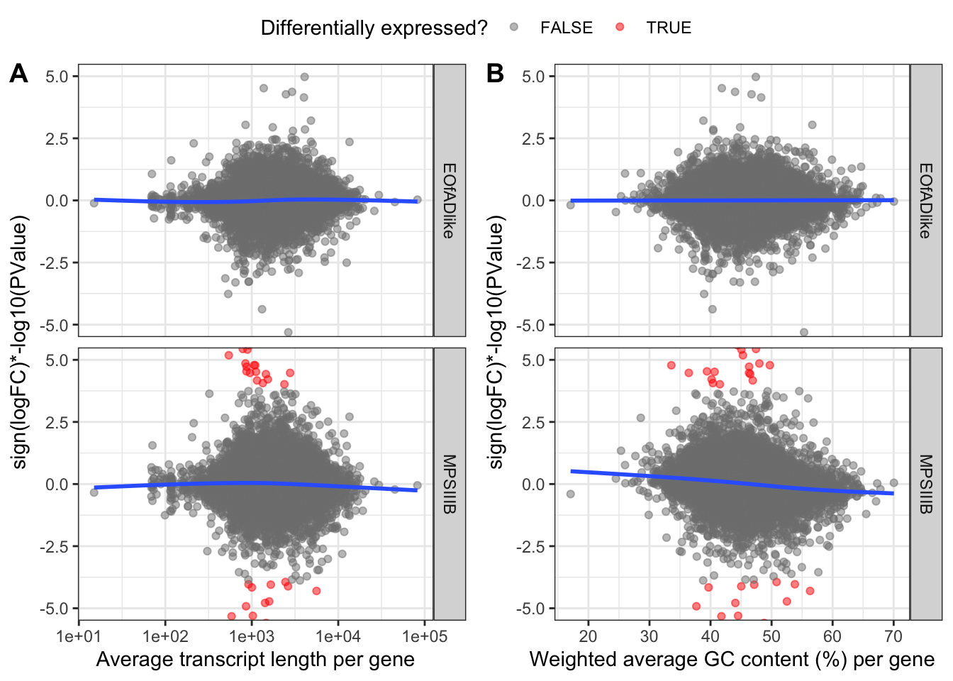
These plots are zoomed in between -10 and 10 on the y-axisfor vis purposes. the blue lines of best fit are a bit wonky, meaning there are some biases here for %GC and Length. Therefore, conditional quantile normailsation is required.

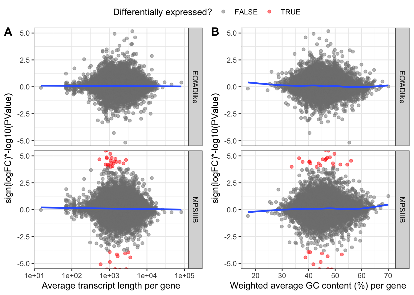
ggarrange(
toptable_1 %>% 
  bind_rows() %>% 
  mutate(rankstat = sign(logFC)*-log10(PValue)) %>% 
  ggplot(aes(x = length, y = rankstat)) +
  geom_point(
    aes(colour = DE),
    alpha = 0.5
  ) +
  geom_smooth(se = FALSE, method = "gam") +
  facet_grid(rows = vars(coef)) +
  theme_bw() +
  theme(legend.position = "none") +
  scale_color_manual(values = c("grey50", "red")) +
  scale_x_log10()+
  labs(x = "Average transcript length per gene",
       colour = "Differentially expressed?",
       y = "sign(logFC)*-log10(PValue)") +
  coord_cartesian(ylim = c(-5, 5)),

toptable_1 %>% 
  bind_rows() %>% 
  mutate(rankstat = sign(logFC)*-log10(PValue)) %>% 
  ggplot(aes(x = gc_content, y = rankstat)) +
  geom_point(
    aes(colour = DE),
    alpha = 0.5
  ) +
  geom_smooth(se = FALSE, method = "gam") +
  facet_grid(rows = vars(coef)) +
  theme_bw() +
  theme(legend.position = "none") +
  scale_color_manual(values = c("grey50", "red")) +
  coord_cartesian(ylim = c(-5,5)) + 
  labs(x = "Weighted average GC content (%) per gene", 
       colour = "Differentially expressed?", 
       y = "sign(logFC)*-log10(PValue)"),
common.legend = TRUE, 
labels = "AUTO"
)

# CQN

A little bit of bias is obsevred for %GC content and gene length, so will apply the cqn correction to adjust for this.

cqn <-   
x %>% 
  with(
    cqn(
      counts = counts,
      x = genes$gc_content,
      lengths = genes$length,
      sizeFactors = samples$lib.size
    )
  )
logCPM <- cqn$y + cqn$offset

plot out the model fits

par(mfrow = c(1, 2))
cqnplot(cqn, n = 1, xlab = "GC Content")
cqnplot(cqn, n = 2, xlab = "Length")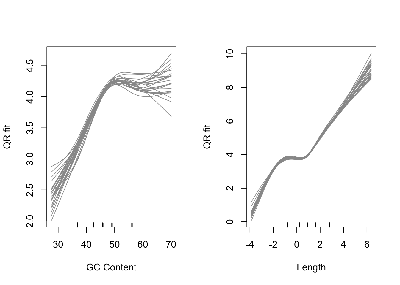

Model fits for GC content and gene length under the CQN model. Variability is clearly visible at either end

par(mfrow = c(1, 1))

PCA after cqn

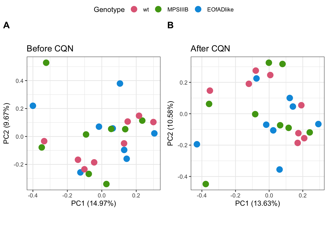
PCA analysis was repeated. No significant improvement of cliustering of samples by genotype is observed

ggarrange(
  cpm(x, log = T) %>%
    t() %>%
    prcomp() %>% 
    autoplot(data = tibble(sample = rownames(.$x)) %>%
               left_join(x$samples),
             colour = "Genotype", 
             
             size = 4
    ) +
    scale_color_discrete_qualitative(palette = "Dark 3") +
    theme(aspect.ratio = 1) +
    ggtitle("Before CQN"),
  
  logCPM %>% 
    t() %>% 
    prcomp() %>%
    autoplot(data = tibble(sample = rownames(.$x)) %>%
               left_join(x$samples),
             colour = "Genotype", 
             size = 4
    ) +
    scale_color_discrete_qualitative(palette = "Dark 3") +
    theme(aspect.ratio = 1) +
    ggtitle("After CQN"),
  common.legend = T, 
  labels = "AUTO"
)

DE with cqn

The DE analysis was then repeated, this time including the offset generated by cqn in the model.

# Add the offset to the dge object 
x$offset <- cqn$glm.offset

# fit the glm
fit_cqn <- x %>% 
  estimateDisp(design) %>% 
  glmFit(design)

toptables_cqn <- design %>% colnames() %>% .[2:3] %>% 
  sapply(function(x){
    glmLRT(fit_cqn, coef = x) %>%
      topTags(n = Inf) %>%
      .[["table"]] %>%
      as_tibble() %>%
      arrange(PValue) %>%
       mutate(
        coef = x,
        DE = FDR < 0.05
      ) %>% 
      dplyr::select(
        gene_name, logFC, logCPM, PValue, FDR, DE, everything()  
      )
      
  }, simplify = FALSE)

Vis

rech-check the rank-stat

ggarrange(
toptables_cqn %>% 
  bind_rows() %>% 
  mutate(rankstat = sign(logFC)*-log10(PValue)) %>% 
  ggplot(aes(x = length, y = rankstat)) +
  geom_point(
    aes(colour = DE),
    alpha = 0.5
  ) +
  geom_smooth(se = FALSE, method = "gam") +
  facet_grid(rows = vars(coef)) +
  theme_bw() +
  theme(legend.position = "none") +
  scale_color_manual(values = c("grey50", "red")) +
  scale_x_log10()+
  labs(x = "Average transcript length per gene",
       colour = "Differentially expressed?",
       y = "sign(logFC)*-log10(PValue)") +
  coord_cartesian(ylim = c(-5, 5)),

toptables_cqn %>% 
  bind_rows() %>% 
  mutate(rankstat = sign(logFC)*-log10(PValue)) %>% 
  ggplot(aes(x = gc_content, y = rankstat)) +
  geom_point(
    aes(colour = DE),
    alpha = 0.5
  ) +
  geom_smooth(se = FALSE, method = "gam") +
  facet_grid(rows = vars(coef)) +
  theme_bw() +
  theme(legend.position = "none") +
  scale_color_manual(values = c("grey50", "red")) +
  coord_cartesian(ylim = c(-5,5)) + 
  labs(x = "Weighted average GC content (%) per gene", 
       colour = "Differentially expressed?", 
       y = "sign(logFC)*-log10(PValue)"),
common.legend = TRUE, 
labels = "AUTO"
)

Gene set enrichment analysis

I now will perform some gene set enrichment analyses on MSIGDB gene sets.

Gene sets

KEGG <- msigdbr("Danio rerio", category = "C2", subcategory = "CP:KEGG") %>% 
  left_join(x$genes, by = c("gene_symbol" = "gene_name")) %>% 
  dplyr::filter(gene_id %in% rownames(x)) %>% 
  distinct(gs_name, gene_id, .keep_all = TRUE) %>% 
  split(f = .$gs_name) %>%
  lapply(extract2, "gene_id")



# GO Terms
goSummaries <- url("https://uofabioinformaticshub.github.io/summaries2GO/data/goSummaries.RDS") %>%
  readRDS() %>%
  mutate(
    Term = Term(id),
    gs_name = Term %>% str_to_upper() %>% str_replace_all("[ -]", "_"),
    gs_name = paste0("GO_", gs_name)
    )

minPath <- 3

GO <-
  msigdbr("Danio rerio", category = "C5") %>%
  dplyr::filter(grepl(gs_name, pattern = "^GO")) %>%
  left_join(x$genes, by = c("gene_symbol" = "gene_name")) %>%
  dplyr::filter(gene_id %in% rownames(x)) %>%
  mutate(gs_name = str_replace(gs_name, pattern = "GOBP_", replacement = "GO_")) %>%
  mutate(gs_name = str_replace(gs_name, pattern = "GOMF_", replacement = "GO_")) %>%
  mutate(gs_name = str_replace(gs_name, pattern = "GOCC_", replacement = "GO_")) %>%
  left_join(goSummaries) %>%
  dplyr::filter(shortest_path >= minPath) %>%
  distinct(gs_name, gene_id, .keep_all = TRUE) %>%
  split(f = .$gs_name) %>%
  lapply(extract2, "gene_id")
 
sizes_GO <- GO %>%
  lapply(length) %>%
  unlist %>%
  as.data.frame() %>%
  set_colnames( "n_genes") %>%
  rownames_to_column("gs")


# retain gene sets with at least 3 genes in it
GO <- GO[sizes_GO %>% dplyr::filter(n_genes > 3) %>% .$gs]

ireGenes <- readRDS("data/gene_sets/zebrafishireGenes.rds") %>% 
  unlist() %>% 
  as.data.frame() %>% 
  rownames_to_column("ire") %>% 
  as_tibble() %>% 
  mutate(ire = str_extract(ire, pattern = "ire[:digit:]_[:alpha:]+")) %>% 
  set_colnames(c("ire", "gene_id")) %>% 
  dplyr::filter(gene_id %in% rownames(x)) %>% 
  split(f = .$ire) %>% 
  lapply(magrittr::extract2,"gene_id") 

chr <- x$genes %>% 
  dplyr::select(gene_id, chromosome) %>% 
  split(f = .$chromosome) %>%
  lapply(extract2, "gene_id") %>% 
  .[c("MT", seq(1:25))] # omit the ALT chromosmes and scaffolds

# Cell type markers for zerbafish 
cell_type_markers <- read_excel("data/gene_sets/1-s2.0-S0012160619304919-mmc7.xlsx") %>% 
  dplyr::filter(grepl(`Day of Origin`, pattern = 5 )) %>%  # restrict to only 5dpf
  dplyr::select(Tissue, 9:24) %>% 
  split(f = .$Tissue) %>% 
  lapply(function(y) {
    y %>% 
      dplyr::select(-Tissue) %>% 
      gather %>% 
      dplyr::select(value) %>% 
      set_colnames("gene_name") %>% 
      left_join(x$genes) %>% 
      na.omit %>% 
      .$gene_id
  }) 

# get length of gene sets
sizes <- cell_type_markers %>% 
  lapply(length) %>% 
  unlist %>% 
  as.data.frame() %>% 
  set_colnames( "n_genes") %>% 
  rownames_to_column("gs")

# retain gene sets with at least 10 genes in it
cell_type_markers <- cell_type_markers[sizes %>% dplyr::filter(n_genes > 5) %>% .$gs]

GOSEQ

First, I will test for over-representation of GO terms within the DE genes. I will do this using goseq as it allows you to include a co-variate which is nice. Since there seems to still be a little bit of bias remaining for %GC content even after cqn, this is what I will speify as the covariate.

There were no DEGs in the EOfAD like mutatns, so no GO testing will be performed for this comparison.

The top 10 GO terms over-represented in the DEGs in MPS-IIIB are plotted below.

pwf <- toptables_cqn$MPSIIIB %>%
      with(
        nullp(
          DEgenes = structure(DE, names = gene_id), 
          bias.data = gc_content
        )
      )

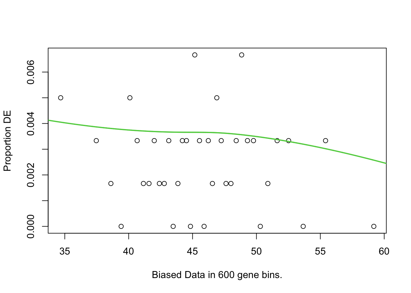
goseq_mpsiiib <- goseq(pwf, gene2cat = GO) %>% 
  as_tibble() %>% 
  dplyr::filter(numDEInCat > 0) %>% 
  mutate(FDR = p.adjust(over_represented_pvalue, method = "fdr")) %>% 
  dplyr::select(-under_represented_pvalue) 

goseq_mpsiiib %>%
  dplyr::slice(1:10) %>%
  mutate(propDE = numDEInCat/numInCat) %>%
  ggplot(aes(x = -log10(over_represented_pvalue), y = reorder(category, -over_represented_pvalue))) +
  geom_col(aes(fill = propDE, alpha = FDR < 0.05)) +
  scale_fill_viridis_c() +
  scale_alpha_manual(values = c(0.4, 1)) +
  labs(y = "GO Term",
       fill = "Proportion of \nDE genes in \nGO term")

Ranked list with fry

Overrepresenation analysis using goseq relies on a hard threshold for gene to be called DE. This can lose information as there are genes which are almost DE (i.e. FDRp = 0.06), but are not interpreted in this way.

Another method to test for enrichment of gene sets is to use ROAST. Roast uses a rotation-based approach to generate a null distribution of gene set enrichment scores by randomly permuting the samples or the gene labels in the data. Roast then calculates a gene set enrichment score for each gene set in the data, based on the correlation between the gene expression values and the sample labels. The gene set enrichment scores are compared to the null distribution to calculate the statistical significance of the enrichment. In this way, it does not requre a list of DEGs as input.

Here, I will perform the fast approx of ROAST: fry, frmo the limma package on the KEGG gene sets. The top 10 gene sets in each mutant zebrafish are shown below.

KEGG

fryKEGG <- 
  design %>% colnames() %>% .[2:3] %>% 
  sapply(function(y) {
   logCPM %>% 
      fry(
        index = KEGG,
        design = design, 
        contrast = y, 
        sort = "mixed"
      ) %>% 
      rownames_to_column("pathway") %>% 
      as_tibble() %>% 
      mutate(coef = y)
  }, simplify = FALSE)

fryKEGG$MPSIIIB %>% 
  dplyr::slice(1:10) %>% 
  mutate(pathway = str_remove(pathway, pattern = "KEGG_")) %>% 
  ggplot(aes(x = -log10(PValue.Mixed), y = reorder(pathway, -PValue.Mixed))) +
  geom_col(aes(fill = FDR.Mixed < 0.05)) +
  scale_fill_manual(values = c("grey50", 'red')) +
  theme_pubr() +
  labs(fill = "FDR < 0.05", 
       x = "-log10(PValue)", 
       y = "", 
       title = "MPS-IIIB")

  #theme(text = element_text(size = 40)) 
  # ggsave("output/plots/geneSetsInMPS-IIIB.png", width = 10, height = 7, 
  #        units = "cm", dpi = 300, scale= 5)
  

fryKEGG$EOfADlike %>% 
  dplyr::slice(1:10) %>% 
  mutate(pathway = str_remove(pathway, pattern = "KEGG_")) %>% 
  ggplot(aes(x = -log10(PValue.Mixed), y = reorder(pathway, -PValue.Mixed))) +
  geom_col(aes(fill = FDR.Mixed < 0.05)) +
  scale_fill_manual(values = c("grey50", 'red')) +
  theme_pubr() +
  labs(fill = "FDR < 0.05", 
       x = "-log10(PValue)", 
       y = "", 
       title = "EOfAD")

GO

Gene ontologies.

fry_GO <-  design %>% colnames() %>% .[2:3] %>% 
  sapply(function(y) {
    logCPM %>% 
      fry(
        index = GO,
        design = design, 
        contrast = y, 
        sort = "mixed"
      ) %>% 
      rownames_to_column("pathway") %>% 
      as_tibble() %>% 
      mutate(coef = y, 
             sig = FDR.Mixed < 0.05)
  }, simplify = FALSE)

sigGOs <- fry_GO %>% 
  bind_rows() %>% 
  dplyr::filter(sig == TRUE) %>% 
  .$pathway

fry_GO %>% 
  bind_rows() %>% 
  dplyr::filter(pathway %in% sigGOs) %>% 
  arrange(desc(coef), PValue.Mixed) %>% 
  mutate(order = rownames(.)) %>% 
  ggplot(aes(x = coef, y = pathway)) +
  geom_tile(
    aes(fill = -log10(PValue.Mixed))
    ) +
  theme_pubr() +
  scale_fill_viridis_c(option = "magma") +
  labs(fill = "-log10(PValue)", 
       x = "", 
       y = "", 
       title = "MPS-IIIB")

  theme(text = element_text(size = 25))

List of 1
 $ text:List of 11
  ..$ family       : NULL
  ..$ face         : NULL
  ..$ colour       : NULL
  ..$ size         : num 25
  ..$ hjust        : NULL
  ..$ vjust        : NULL
  ..$ angle        : NULL
  ..$ lineheight   : NULL
  ..$ margin       : NULL
  ..$ debug        : NULL
  ..$ inherit.blank: logi FALSE
  ..- attr(*, "class")= chr [1:2] "element_text" "element"
 - attr(*, "class")= chr [1:2] "theme" "gg"
 - attr(*, "complete")= logi FALSE
 - attr(*, "validate")= logi TRUE

  # ggsave("output/plots/gotermsMPS-IIIB.png", width = 10, height = 7, 
  #        units = "cm", dpi = 300, scale= 5)
  

fry_GO$EOfADlike %>% 
  dplyr::slice(1:32) %>% 
  ggplot(aes(x = -log10(PValue.Mixed), y = reorder(pathway, -PValue.Mixed))) +
  geom_col(aes(fill = -log10(PValue.Mixed))) +
  scale_fill_viridis_c() +
  theme_pubr() +
  labs(fill = "FDR < 0.05", 
       x = "-log10(PValue)", 
       y = "", 
       title = "MPS IIIB")

  ggsave("output/plots/gotermsMPS-IIIB.png", width = 10, height = 5, 
         units = "cm", dpi = 300, scale= 4)

IRE

Statistical significance in these iron-responsive element gene sets can indicate iron dyshomoestasis.

fryIRE <- design %>% colnames() %>% .[2:3] %>% 
  sapply(function(y) {
    cpm(x$counts, log = TRUE) %>% 
      fry(
        index = ireGenes,
        design = design, 
        contrast = y, 
        sort = "directional"
      ) %>% 
      rownames_to_column("pathway") %>% 
      as_tibble() %>% 
      mutate(coef = y)
  }, simplify = FALSE)

fryIRE %>% 
  bind_rows() %>% 
  dplyr::select(pathway, coef, pvalue = PValue.Mixed, FDR = FDR.Mixed) %>% 
  ggplot(aes(y = pathway, x = -log10(pvalue))) + 
  geom_col(aes(fill = coef), 
           position = "dodge") +
  geom_vline(xintercept = -log10(0.05)) +
  scale_fill_viridis_d(end = 0.75) +
  theme_pubr()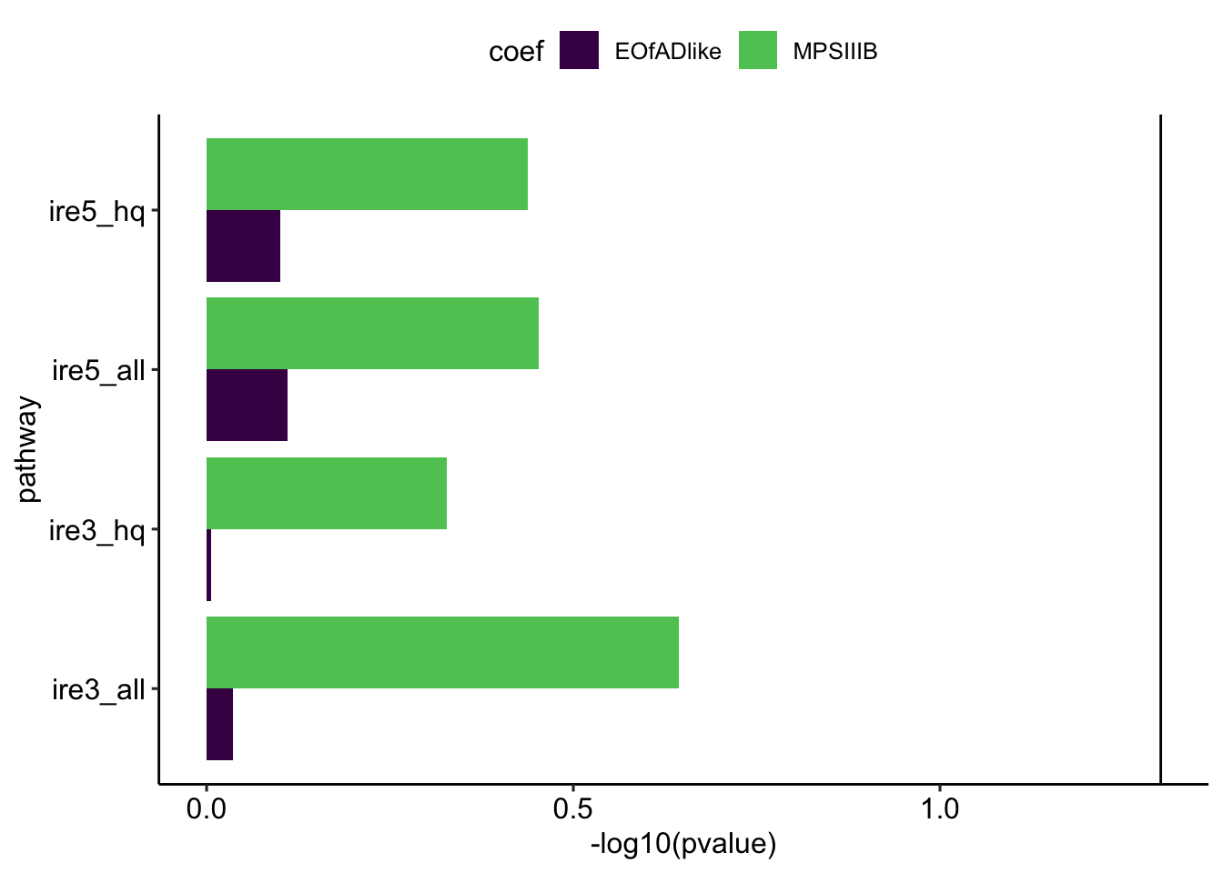

  #ggsave("output/plots/ire.png", width = 10, height = 10, units = "cm", dpi = 300)

Cell type prop check

Since this experiment was performed on whole larvae, we need to have a look at whether changes to cell type proportions could explain cause some artefactual changes to gene expression. We have done this previously by assessing the expression of marker genes of specific cell types. So this is what I will do here. I have taken the lists of genes frmo day 5 only from the zebrafish single cell atlas (Farnsworth et al. 2020) which contain at least 10 genes. This leaves 24 gene sets (cell types) to test.

fry.cell <- design %>% colnames() %>% .[2:3] %>% 
  sapply(function(y) {
    cpm(x$counts, log = TRUE) %>% 
      fry(
        index = cell_type_markers,
        design = design, 
        contrast = y, 
        sort = "directional"
      ) %>% 
      rownames_to_column("pathway") %>% 
      as_tibble() %>% 
      mutate(coef = y) %>% 
      dplyr::select(1:5)
  }, simplify = FALSE)

Chromosome gene sets

Are there DEGs on the mutant chromosomes?

design %>% colnames() %>% .[2:3] %>% 
  sapply(function(y) {
    cpm(x$counts, log = TRUE) %>% 
      fry(
        index = c(chr),
        design = design, 
        contrast = y, 
        sort = "mixed"
      ) %>% 
      rownames_to_column("pathway") %>% 
      as_tibble() %>% 
      mutate(coef = y)
  }, simplify = FALSE)

$MPSIIIB
# A tibble: 26 × 8
   pathway NGenes Direction PValue   FDR PValue.Mixed     FDR.Mixed coef   
   <chr>    <int> <chr>      <dbl> <dbl>        <dbl>         <dbl> <chr>  
 1 24         615 Up        0.258  0.280     2.44e-10 0.00000000634 MPSIIIB
 2 25         665 Up        0.0147 0.179     3.25e- 3 0.0423        MPSIIIB
 3 8          939 Up        0.115  0.179     1.40e- 1 0.508         MPSIIIB
 4 5         1219 Up        0.0729 0.179     1.75e- 1 0.508         MPSIIIB
 5 17         819 Up        0.115  0.179     1.81e- 1 0.508         MPSIIIB
 6 14         763 Up        0.122  0.179     1.94e- 1 0.508         MPSIIIB
 7 3         1176 Up        0.166  0.188     2.12e- 1 0.508         MPSIIIB
 8 15         825 Up        0.101  0.179     2.36e- 1 0.508         MPSIIIB
 9 12         770 Up        0.160  0.188     2.36e- 1 0.508         MPSIIIB
10 11         734 Up        0.138  0.179     2.41e- 1 0.508         MPSIIIB
# ℹ 16 more rows

$EOfADlike
# A tibble: 26 × 8
   pathway NGenes Direction PValue   FDR PValue.Mixed FDR.Mixed coef     
   <chr>    <int> <chr>      <dbl> <dbl>        <dbl>     <dbl> <chr>    
 1 17         819 Up         0.781 0.846        0.226     0.986 EOfADlike
 2 18         697 Up         0.557 0.752        0.473     0.986 EOfADlike
 3 9          817 Up         0.474 0.752        0.513     0.986 EOfADlike
 4 25         665 Up         0.237 0.752        0.548     0.986 EOfADlike
 5 23         834 Up         0.613 0.752        0.643     0.986 EOfADlike
 6 2         1055 Up         0.577 0.752        0.661     0.986 EOfADlike
 7 3         1176 Up         0.631 0.752        0.696     0.986 EOfADlike
 8 4         1084 Down       0.986 0.990        0.799     0.986 EOfADlike
 9 8          939 Up         0.689 0.779        0.874     0.986 EOfADlike
10 14         763 Up         0.636 0.752        0.874     0.986 EOfADlike
# ℹ 16 more rows

Harmonic mean p

Since I’m not detecting any significant gene sets in the EOfAD-like mutants, I need to try another method. I will use the harmonic mean p val method which combines indivisual p vals from 3 gene set enrichmen analysis methods: fry, camera and gsea.

# Make a custom function for calculating the HMP.  
runHMP = function(gene.set.obj, 
                  design,
                  logCPM.df, 
                  toptable) {
fry <- 
  design %>% colnames() %>% .[2:3] %>% 
  sapply(function(y) {
  logCPM.df %>% 
      fry(
        index = gene.set.obj,
        design = design, 
        contrast = y, 
        sort = "mixed"
      ) %>% 
      rownames_to_column("pathway") %>% 
      as_tibble() %>% 
      mutate(coef = y)
  }, simplify = FALSE)

camera <- 
  design %>% colnames() %>% .[2:3] %>% 
  sapply(function(y) {
    logCPM.df %>% 
      camera(
        index = gene.set.obj,
        design = design, 
        contrast = y
      ) %>% 
      rownames_to_column("pathway") %>% 
      as_tibble() %>% 
      mutate(coef = y)
  }, simplify = FALSE)

ranks <- 
   sapply(toptable, function(y) {
     y %>% 
       mutate(rankstat = sign(logFC) * log10(1/PValue)) %>% 
       arrange(rankstat) %>% 
       dplyr::select(c("gene_id", "rankstat")) %>% #only want the Pvalue with sign
       with(structure(rankstat, names = gene_id)) %>% 
       rev() # reverse so the start of the list is upregulated genes
   }, simplify = FALSE)

# Run fgsea

# set a seed for a reproducible result
set.seed(33)
fgsea <- ranks %>%
  sapply(function(x){
    fgseaMultilevel(stats = x, pathways = gene.set.obj) %>%
      as_tibble() %>%
      dplyr::rename(FDR = padj) %>%
      mutate(padj = p.adjust(pval, "bonferroni")) %>%
      dplyr::select(pathway, pval, FDR, padj, everything()) %>%
      arrange(pval) %>%
      mutate(sig = padj < 0.05)
  }, simplify = F)

fgsea$MPSIIIB %<>% 
  mutate(coef = "MPSIIIB")
fgsea$EOfADlike %<>% 
  mutate(coef = "EOfADlike")

hmp <- fry %>% 
  bind_rows() %>% 
  dplyr::select(pathway, PValue.Mixed, coef) %>% 
  dplyr::rename(fry_p = PValue.Mixed) %>% 
  left_join(camera %>% 
              bind_rows() %>% 
              dplyr::select(pathway, PValue, coef), 
            by = c("pathway", "coef")) %>% 
  dplyr::rename(camera_p = PValue) %>% 
  left_join(fgsea %>% 
              bind_rows() %>% 
              dplyr::select(pathway, pval, coef), 
            by = c("pathway", "coef")) %>% 
  dplyr::rename(fgsea_p = pval) %>% 
  bind_rows() %>% 
  nest(p = one_of(c("fry_p", "camera_p", "fgsea_p"))) %>% 
 mutate(harmonic_p = vapply(p, function(x){
        x <- unlist(x)
        x <- x[!is.na(x)]
        p.hmp(x, L = 4)
      }, numeric(1))
 ) %>% 
  unnest() %>% 
  mutate(harmonic_p_FDR = p.adjust(harmonic_p, "fdr"),
         sig = harmonic_p_FDR < 0.05) %>% 
  arrange(harmonic_p) 

return(list(
  hmp = hmp, 
  fgsea = fgsea
))

}

KEGG

HMP_kegg <- runHMP(gene.set.obj = KEGG, 
                   design = design, 
                   logCPM.df = logCPM, 
                   toptable = toptables_cqn)

sigpaths <- HMP_kegg$hmp %>% 
  dplyr::filter(harmonic_p_FDR < 0.05) %>% 
  .$pathway

HMP_kegg$hmp %>% 
  dplyr::filter(pathway %in% sigpaths) %>% 
  ggplot(aes(x = coef, y = reorder(pathway, -harmonic_p))) + 
  geom_tile(aes(fill = -log10(harmonic_p), 
                alpha = sig)) +
  geom_label(aes(label = signif(harmonic_p_FDR, digits = 2)), 
             fill = NA) +
  scale_fill_viridis_c()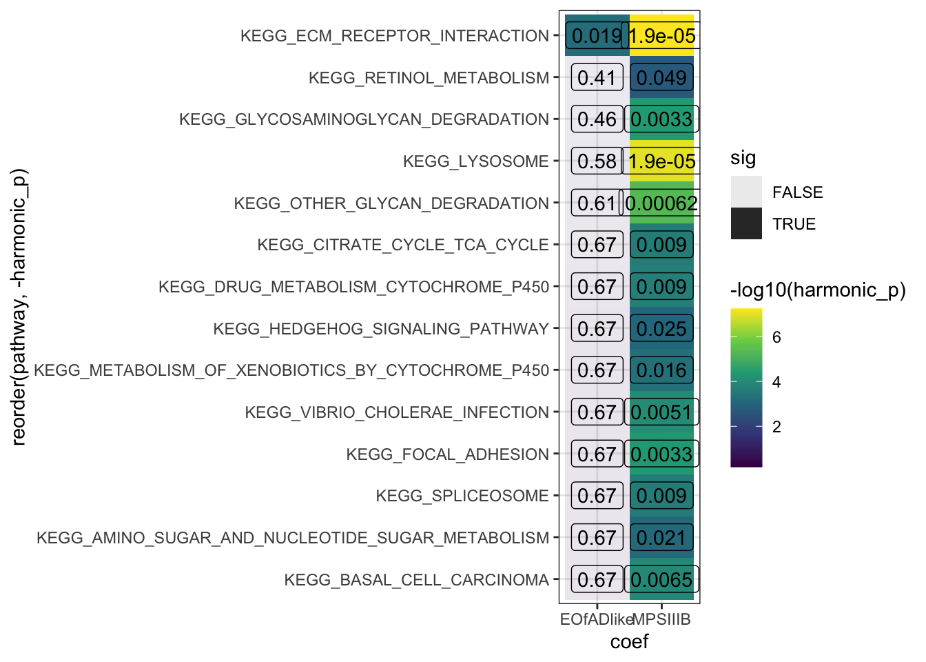

IRE

No staistical significance in the IRE genes

HMP_ire <- runHMP(gene.set.obj = ireGenes, 
                   design = design, 
                   logCPM.df = logCPM, 
                   toptable = toptables_cqn)


HMP_ire$hmp %>% 
  ggplot(aes(x = coef, y = reorder(pathway, -harmonic_p))) + 
  geom_tile(aes(fill = -log10(harmonic_p), 
                alpha = sig)) +
  geom_label(aes(label = signif(harmonic_p_FDR, digits = 2)), 
             fill = NA) +
  scale_fill_viridis_c()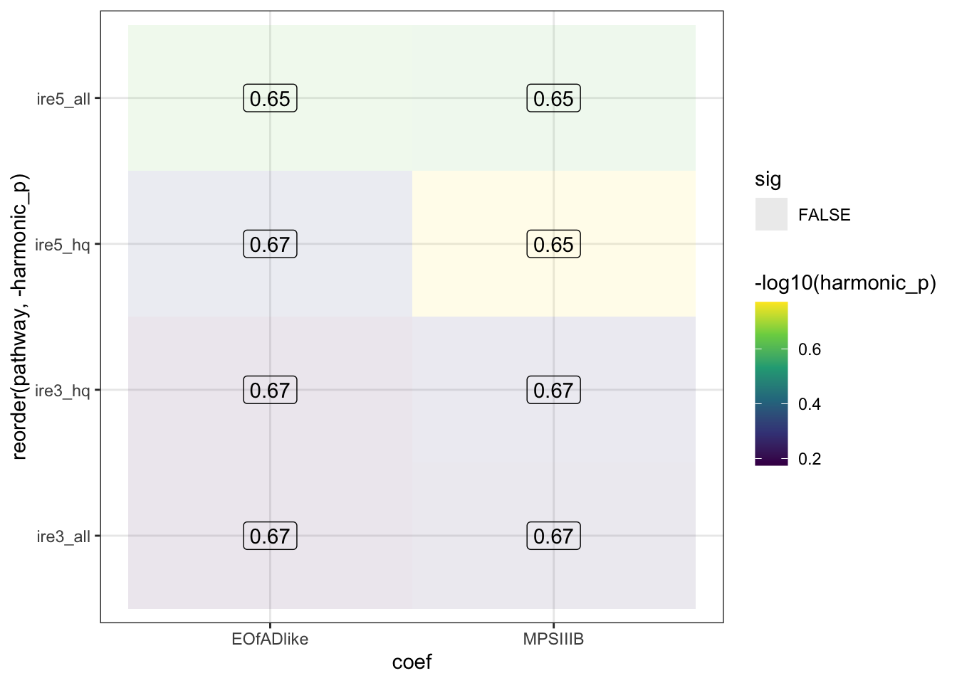

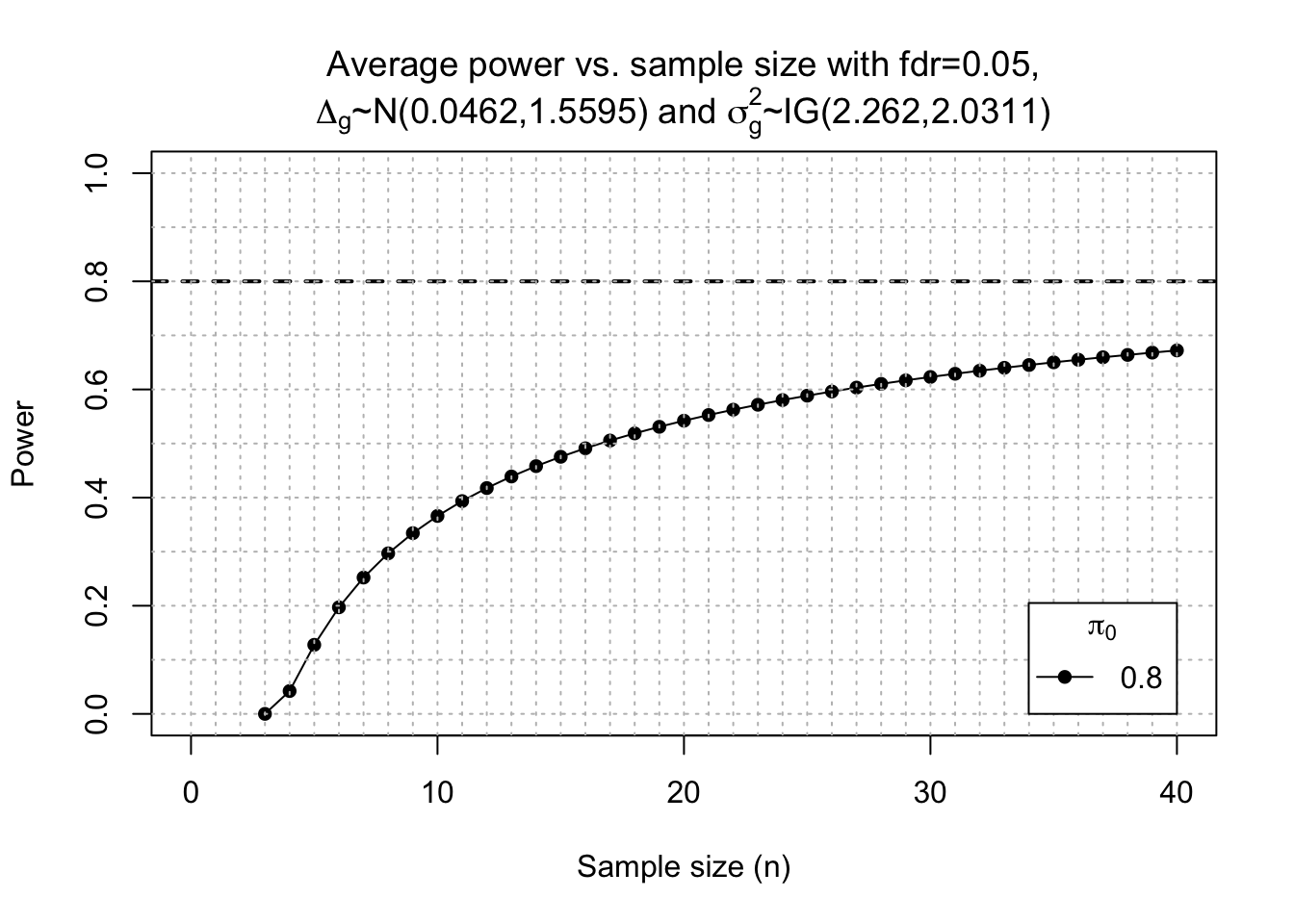
Post-hoc power calc

set.seed(2016)

mu <- x$counts %>%
  as.data.frame() %>%
  .[grepl(colnames(x$counts), pattern = "wt")] %>%
  rowMeans()

disp <-  x %>% estimateDisp() %>% . $tagwise.dispersion

fc <- function(y){exp(rnorm(y, log(1), 0.5*log(2)))}

power <- ssizeRNA_vary(nGenes = dim(x)[1], # Num detectable genes
              pi0 = 0.9, # Proportion of non-DE genes
              m = 30, # pseudo sample size
              mu = mu, # Average read count for each gene in control group. Calculated from this current dataset)
              disp = disp, # Dispersion parameter for each gene
              fc = fc, # Fold change per gene
              fdr = 0.05, # FDR level to control
              #power = 0.7, # power level
              maxN = 40,
              replace = T
                )

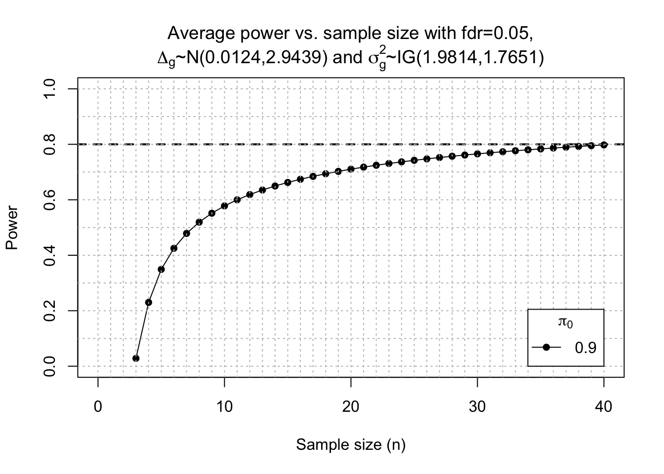
power$power %>% 
  set_colnames(c("n", "power")) %>% 
  ggplot(aes(x = n, y = power)) +
  geom_point() +
  geom_line() +
  coord_cartesian(xlim = c(0,30)) +
  geom_hline(yintercept = 0.7, linetype = 2, colour = "red") +
  geom_hline(yintercept = 0.51, linetype = 2, colour = "blue")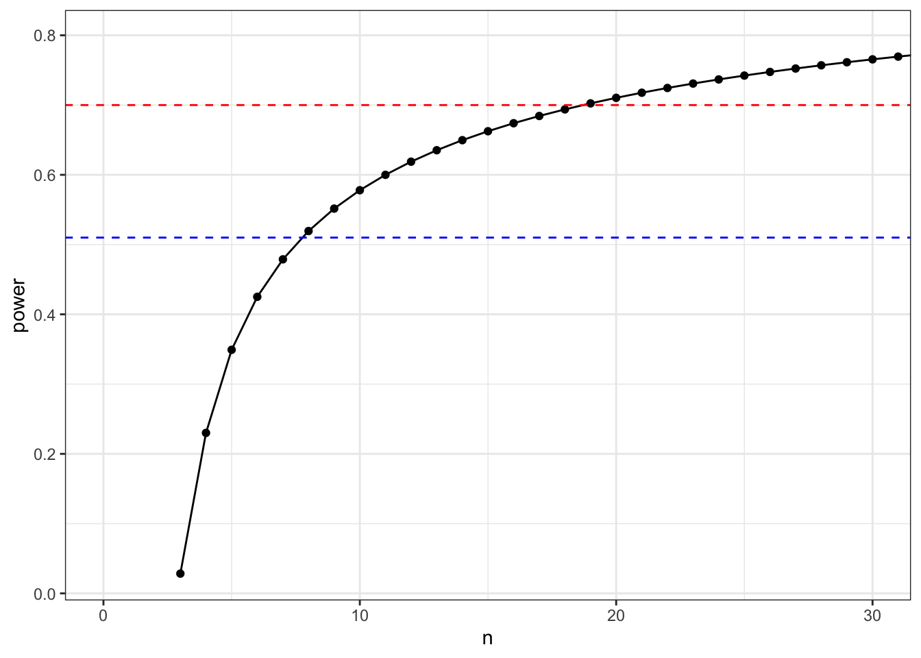

  #ggsave("output/plots/posthocPowerLarvae.png", width = 10, height = 5, units = "cm", 
   #      dpi = 200, scale = 1.5)

Compare with Dong et al. data

Yang had previously analysed the EOfADlike mutation in pools of larvae. Here, I want to see how similar my results are.

Obtained his github repo from here, which has the data https://github.com/yangdongau/20190717_Lardelli_RNASeq_Larvae

Comparing his fc vales im not really seeing much. I wil re-process his data to do HMP analyses on it.

x.Dong <- read_rds("data/DongEtAlData/dgeList.rds")

x.Dong$samples %<>% 
  mutate(Genotype = case_when(
    Genotype == "Q96K97del/+" ~ "EOfADlike", 
    Genotype == "WT" ~ "wt"
  ) %>% 
    factor(levels = c("wt", "EOfADlike")))

larvaeGenos <- x.Dong$samples %>% 
  dplyr::select(Genotype) %>% 
  mutate(exp = "pools") %>% 
  bind_rows(x$samples %>% dplyr::select(Genotype) %>% mutate(exp = "individual")) %>% 
  rownames_to_column("sample")

# PCA
cpm(x, log = T) %>% 
  as.data.frame() %>% 
  rownames_to_column("gene_id") %>% 
  left_join(x.Dong$counts %>% cpm(log=T) %>% as.data.frame %>% rownames_to_column("gene_id")) %>% 
  column_to_rownames("gene_id") %>% 
  dplyr::select(!starts_with("MPS")) %>% 
  na.omit %>% 
  t %>% 
  prcomp() %>% 
  autoplot(data = tibble(sample = rownames(.$x)) %>%
             left_join(larvaeGenos),
           colour = "Genotype", 
           size = 4
  ) +
  geom_mark_ellipse(aes(labels = exp)) +
  scale_color_discrete_qualitative(palette = "Dark 3") +
  theme(aspect.ratio = 1)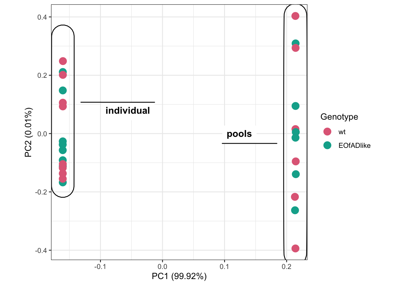

# suss out ECM
toptable_dongetal <- 
  read_csv("data/DongEtAlData/topTable.csv") %>% 
  dplyr::rename( gene_id = ensembl_gene_id, 
                 gene_name = external_gene_name)

toptable_dongetal %>% 
  dplyr::filter(gene_id %in% KEGG$KEGG_ECM_RECEPTOR_INTERACTION) %>% 
  dplyr::select(gene_name, logFC.pools = logFC) %>% 
  left_join(toptables_cqn$EOfADlike %>% dplyr::select(gene_name, logFC.individuals = logFC)) %>% 
  dplyr::distinct(gene_name, .keep_all = T) %>% 
  column_to_rownames("gene_name") %>% 
  pheatmap(color = colorRampPalette(rev(brewer.pal(n = 5,
                                               name = "RdBu")))(200), 
           breaks = seq(-0.6, 0.6, by = 0.6*2/200), 
           main ="KEGG_ECM_RECEPTOR_INTERACTION")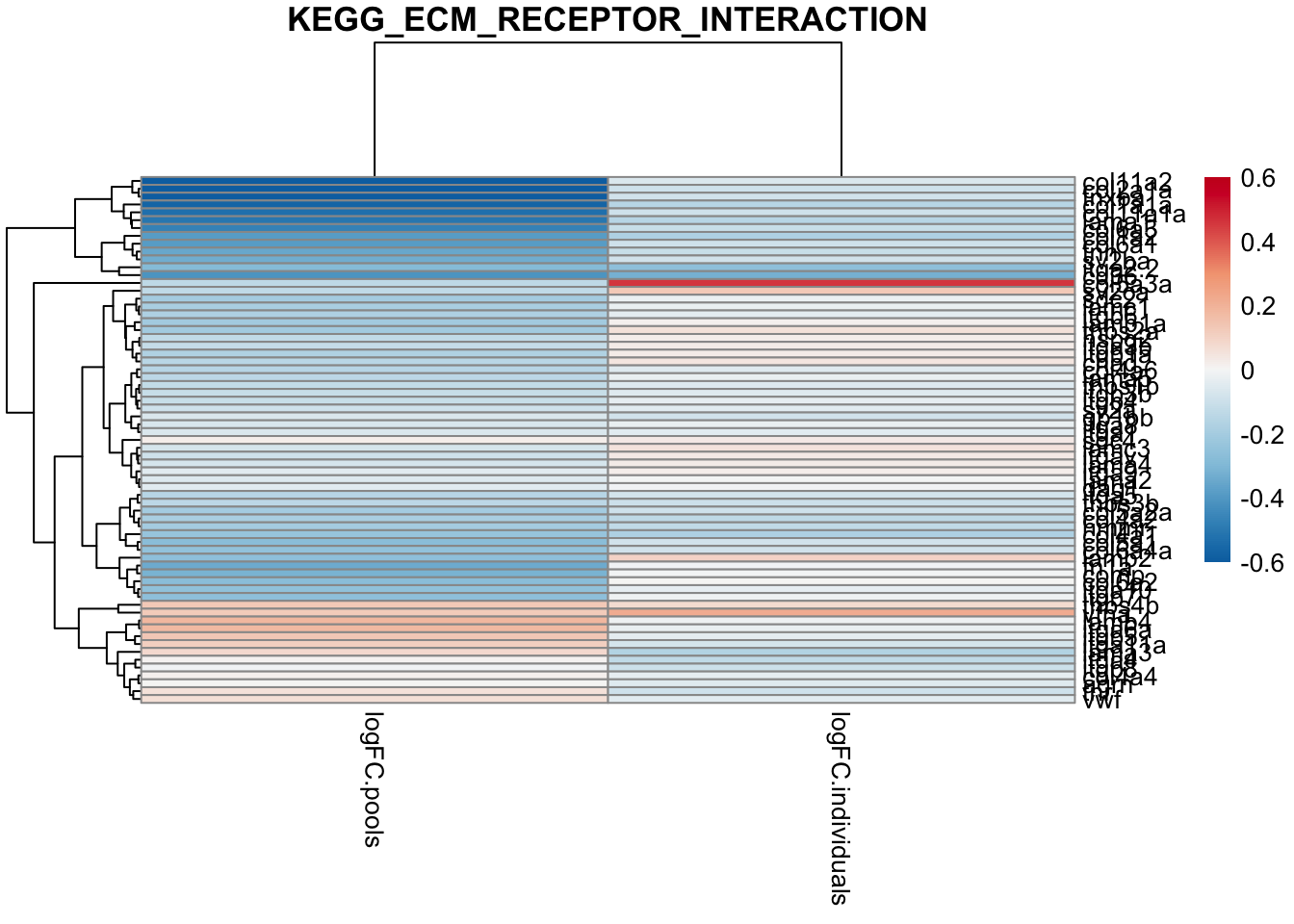

toptable_dongetal %>% 
  dplyr::filter(gene_id %in% KEGG$KEGG_ECM_RECEPTOR_INTERACTION) %>% 
  dplyr::select(gene_name, logFC.pools = logFC) %>% 
    left_join(toptables_cqn$EOfADlike %>% dplyr::select(gene_name, logFC.individuals = logFC)) %>% 
  dplyr::distinct(gene_name, .keep_all = T) %>% 
  column_to_rownames("gene_name") %>% 
  ggscatter(x = "logFC.individuals", y = "logFC.pools",
   color = "black", shape = 21, size = 3, # Points color, shape and size
   add = "reg.line",  # Add regressin line
   add.params = list(color = "blue", fill = "lightgray"), # Customize reg. line
   conf.int = TRUE, # Add confidence interval
   cor.coef = TRUE, # Add correlation coefficient. see ?stat_cor
   #cor.coeff.args = list(method = "pearson", label.x = 3, label.sep = "\n")
   ) +
  geom_abline(slope = 1) +
  labs(title = "Pearson corr of genes in KEGG_ECM_RECEPTOR_INTERACTION")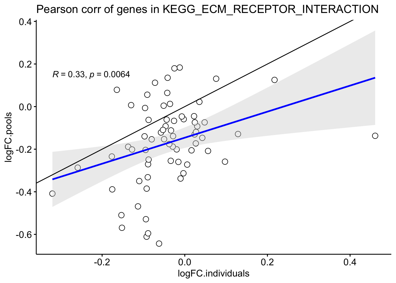

pwf.dong <- toptable_dongetal %>%
      with(
        nullp(
          DEgenes = structure(DE, names = gene_id), 
          bias.data = aveLength 
        )
      )

goseq_dong <- goseq(pwf.dong, gene2cat = GO) %>% 
  as_tibble() %>% 
  #dplyr::filter(numDEInCat > 0) %>% 
  mutate(FDR = p.adjust(over_represented_pvalue, method = "fdr")) %>% 
  dplyr::select(-under_represented_pvalue) 

goseq_dong %>% dplyr::filter(category == "GO_PROTON_TRANSPORTING_V_TYPE_ATPASE_COMPLEX")

# A tibble: 1 × 5
  category                      over_represented_pva…¹ numDEInCat numInCat   FDR
  <chr>                                          <dbl>      <int>    <int> <dbl>
1 GO_PROTON_TRANSPORTING_V_TYP…                      1          0       25     1
# ℹ abbreviated name: ¹over_represented_pvalue

goseq_mpsiiib %>% 
  dplyr::slice(1:10) %>% 
  mutate(propDE = numDEInCat/numInCat) %>% 
  ggplot(aes(x = -log10(over_represented_pvalue), y = reorder(category, -over_represented_pvalue))) +
  geom_col(aes(fill = propDE, alpha = FDR < 0.05)) +
  scale_fill_viridis_c() +
  scale_alpha_manual(values = c(0.4, 1)) +
  labs(y = "GO Term", 
       fill = "Proportion of \nDE genes in \nGO term")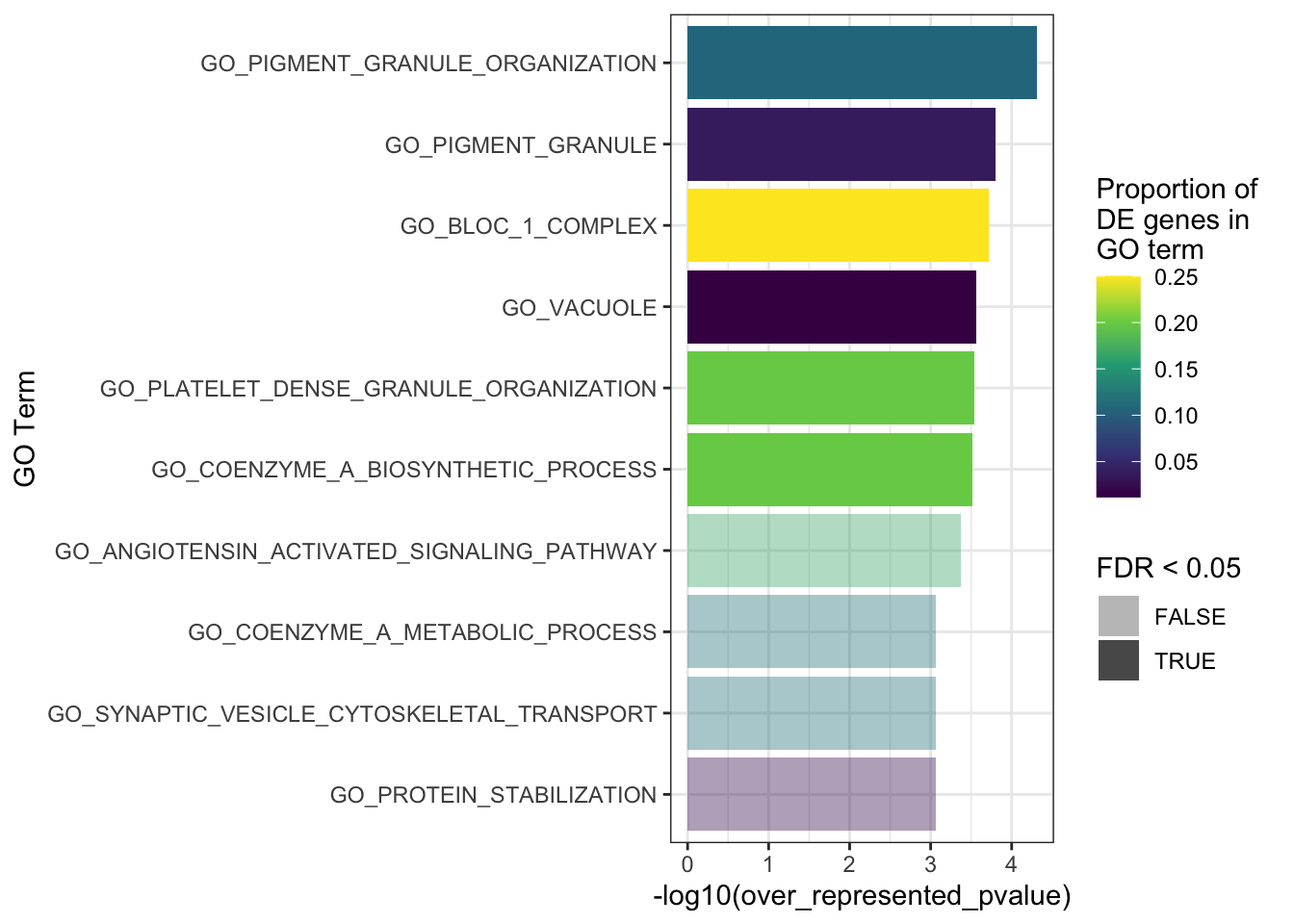

HMP with dong et al.

design.dong <- model.matrix(~Genotype + W_1, x.Dong$samples) %>% 
  set_colnames(str_replace(colnames(.), pattern = "Genotype.+", "EOfAD-like"))

fry <- 
  cpm(x.Dong, log = T) %>% 
      fry(
        index = KEGG,
        design = design.dong, 
        contrast = "EOfAD-like", 
        sort = "mixed"
      ) %>% 
      rownames_to_column("pathway") %>% 
      as_tibble() %>% 
      mutate(coef = "EOfAD-like", 
             sig = FDR.Mixed < 0.05)

camera <- 
  cpm(x.Dong, log = T) %>% 
  camera(
    index = KEGG,
    design = design.dong, 
    contrast = "EOfAD-like"
  ) %>% 
      rownames_to_column("pathway") %>% 
      as_tibble() %>% 
      mutate(coef = "EOfAD-like")

ranks <- 
  toptable_dongetal %>% 
  mutate(rankstat = sign(logFC) * log10(1/PValue)) %>% 
  arrange(rankstat) %>% 
  dplyr::select(c("gene_id", "rankstat")) %>% #only want the Pvalue with sign
  with(structure(rankstat, names = gene_id)) %>% 
  rev() # reverse so the start of the list is upregulated genes

# Run fgsea

# set a seed for a reproducible result
set.seed(33)
fgsea <- ranks %>%
  fgseaMultilevel(pathways = KEGG) %>%
  as_tibble() %>%
  dplyr::rename(FDR = padj) %>%
  mutate(padj = p.adjust(pval, "bonferroni")) %>%
  dplyr::select(pathway, pval, FDR, padj, everything()) %>%
  arrange(pval) %>%
  mutate(sig = padj < 0.05, 
         coef ="EOfAD-like")

hmp.dong <- fry %>% 
  dplyr::select(pathway, PValue.Mixed, coef) %>% 
  dplyr::rename(fry_p = PValue.Mixed) %>% 
  left_join(camera %>% 
              dplyr::select(pathway, PValue, coef), 
            by = c("pathway", "coef")) %>% 
  dplyr::rename(camera_p = PValue) %>% 
  left_join(fgsea %>% 
              bind_rows() %>% 
              dplyr::select(pathway, pval, coef), 
            by = c("pathway", "coef")) %>% 
  dplyr::rename(fgsea_p = pval) %>% 
  bind_rows() %>% 
  nest(p = one_of(c("fry_p", "camera_p", "fgsea_p"))) %>% 
 mutate(harmonic_p = vapply(p, function(x){
        x <- unlist(x)
        x <- x[!is.na(x)]
        p.hmp(x, L = 4)
      }, numeric(1))
 ) %>% 
  unnest() %>% 
  mutate(harmonic_p_FDR = p.adjust(harmonic_p, "fdr"),
         sig = harmonic_p_FDR < 0.05) %>% 
  arrange(harmonic_p) 

hmp.kegg.q96 <- hmp.dong %>% 
  mutate(exp = "pools") %>% 
  bind_rows(HMP_kegg$hmp %>% 
              mutate(exp = "individuals")) %>% 
  dplyr::filter(coef == "EOfADlike")

sig.q96 <- hmp.kegg.q96 %>% 
  dplyr::filter(sig == T) %>% 
  .$pathway %>% 
  unique

hmp.dong %>% 
  dplyr::filter(pathway %in% sig.q96) %>% 
  ggplot(aes(x = -log10(harmonic_p), y = reorder(pathway, -harmonic_p))) +
  geom_col(aes(fill = -log10(harmonic_p))) +
  scale_fill_viridis_c() +
  theme_classic()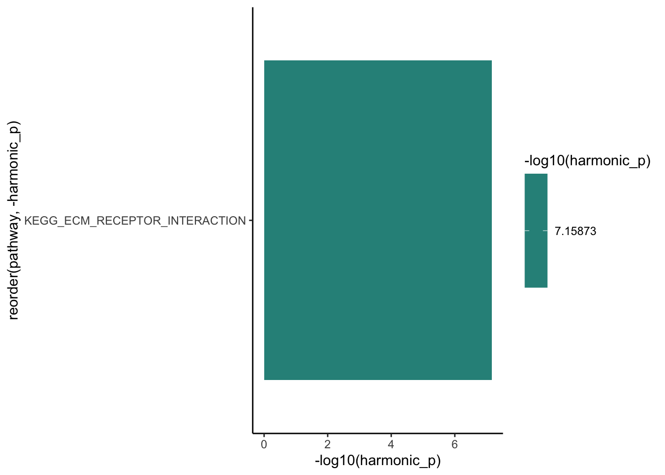

does Genotype drive the Dong ECM?

form <- ~ (1|Genotype) + (1|pair)
geneExpr <- 
  x.Dong$counts #%>% 
    # as.data.frame() %>% 
    # rownames_to_column("gene_id") %>% 
    # dplyr::filter(gene_id %in% KEGG$KEGG_ECM_RECEPTOR_INTERACTION) %>% 
    # column_to_rownames("gene_id")
#
n <- parallel::detectCores()/2 # experiment!
cl <- parallel::makeCluster(n)
doParallel::registerDoParallel(cl)

# this takes forever to run.
#varpar <- fitExtractVarPartModel(geneExpr, form, x.Dong$samples, 
#                                 BPPARAM=SnowParam(1)) # turn off parallel as my laptop sucks
#saveRDS(varpar, "data/dongvarpar.rds")                
varpar <- readRDS("data/dongvarpar.rds")

varpar %>% 
  .[KEGG$KEGG_ECM_RECEPTOR_INTERACTION,] %>% 
  rownames_to_column("gene_id") %>% 
  na.omit %>% 
  arrange(Genotype) %>% 
  gather(key = "var", value = "prop", c(Genotype, pair, Residuals)) %>% 
  ggplot(aes(x = var, y = prop)) +
  geom_violin() +
  geom_boxplot(width = 0.1)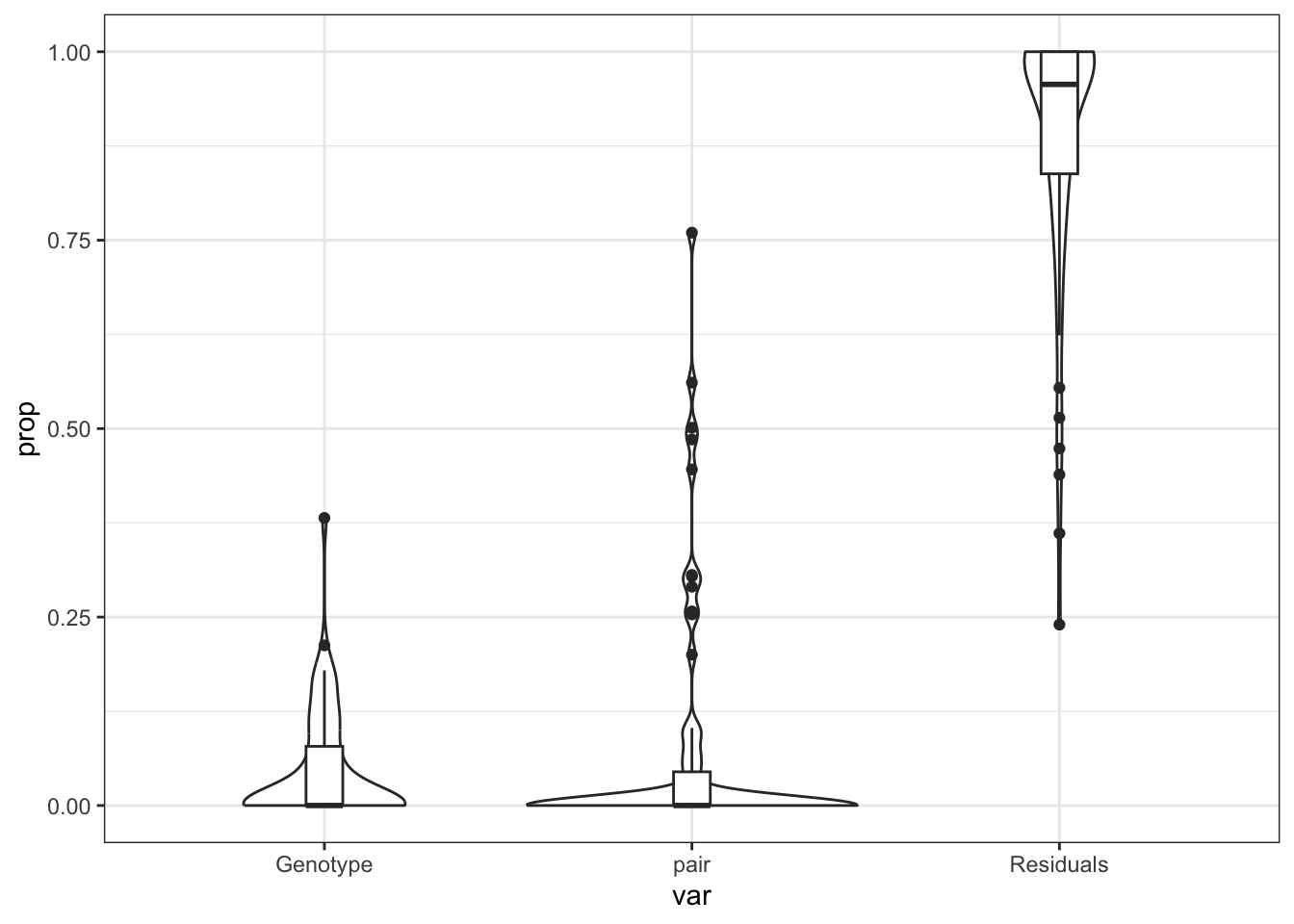

## power calc Dong # Post-hoc power calc

set.seed(2016)

mu2 <- 
  x.Dong$counts %>%
  as.data.frame() %>%
  .[,(x.Dong$samples %>% dplyr::filter(Genotype == "wt") %>% .$sample)] %>%
  rowMeans()

disp2 <-  x.Dong %>% estimateDisp() %>% . $tagwise.dispersion

fc <- function(y){exp(rnorm(y, log(1), 0.5*log(1.5)))}

power2 <- ssizeRNA_vary(nGenes = dim(x.Dong)[1], # Num detectable genes
              pi0 = 0.8, # Proportion of non-DE genes
              m = 30, # pseudo sample size
              mu = mu2, # Average read count for each gene in control group. Calculated from this current dataset)
              disp = disp2, # Dispersion parameter for each gene
              fc = fc, # Fold change per gene
              fdr = 0.05, # FDR level to control
              #power = 0.7, # power level
              maxN = 40,
              replace = T
                )

power2$power %>% 
  set_colnames(c("n", "power")) %>% 
  ggplot(aes(x = n, y = power)) +
  geom_point() +
  geom_line() +
  coord_cartesian(xlim = c(0,30)) +
  geom_vline(xintercept = 8)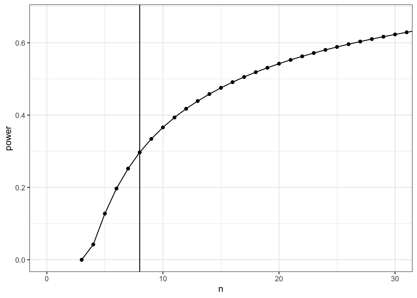

  geom_hline(yintercept = 0.51, linetype = 2, colour = "blue")

mapping: yintercept = ~yintercept 
geom_hline: na.rm = FALSE
stat_identity: na.rm = FALSE
position_identity

  # ggsave("output/plots/posthocPowerLarvae.png", width = 10, height = 5, units = "cm", 
  #        dpi = 200, scale = 1.5)

Data export

x %>% saveRDS("data/R_objects/larvae/dge.rds")
logCPM %>% saveRDS("data/R_objects/larvae/logcpm.rds")
toptables_cqn %>% saveRDS("data/R_objects/larvae/toptablescqn.rds")
HMP_kegg %>% saveRDS("data/R_objects/larvae/hmp_kegg.rds")
HMP_ire %>% saveRDS("data/R_objects/larvae/hmp_ire.rds")
fry.cell %>% saveRDS("data/R_objects/larvae/celltype_larvae.rds")

# 
# ire.output <- HMP_ire$hmp %>% 
#   left_join(HMP_ire$fgsea %>% 
#               bind_rows() %>% 
#               dplyr::select(pathway, coef, leadingEdge),
#             by = c('pathway', 'coef')
#   ) %>% 
#   split(f = .$coef) %>% 
#   lapply(dplyr::select, -coef) %>% 
#   set_names(
#     names(.) %>% 
#       paste0("mRNA_ire_7dpf_", .)
#   )
# 
# KEGG.output <- HMP_kegg$hmp %>% 
#   left_join(HMP_kegg$fgsea %>% 
#               bind_rows() %>% 
#               dplyr::select(pathway, coef, leadingEdge),
#             by = c('pathway', 'coef')
#   ) %>% 
#   split(f = .$coef) %>% 
#   lapply(dplyr::select, -coef) %>% 
#   set_names(
#     names(.) %>% 
#       paste0("mRNA_KEGG_7dpf_", .)
#   )
# 
# c(KEGG.output, ire.output) %>%
#   write.xlsx("output/spreadsheets/RNAseqlarvae_hmpoutputs.xlsx")
# 
# fry.cell %>% 
#   write.xlsx("output/spreadsheets/RNAseqlarvae_celltypeFry.xlsx")

sessionInfo()

R version 4.3.2 (2023-10-31)
Platform: aarch64-apple-darwin20 (64-bit)
Running under: macOS Sonoma 14.3

Matrix products: default
BLAS:   /Library/Frameworks/R.framework/Versions/4.3-arm64/Resources/lib/libRblas.0.dylib 
LAPACK: /Library/Frameworks/R.framework/Versions/4.3-arm64/Resources/lib/libRlapack.dylib;  LAPACK version 3.11.0

locale:
[1] en_US.UTF-8/en_US.UTF-8/en_US.UTF-8/C/en_US.UTF-8/en_US.UTF-8

time zone: Australia/Adelaide
tzcode source: internal

attached base packages:
[1] stats4    splines   stats     graphics  grDevices utils     datasets 
[8] methods   base     

other attached packages:
 [1] ensembldb_2.26.0         AnnotationFilter_1.26.0  GenomicFeatures_1.54.4  
 [4] AnnotationDbi_1.64.1     Biobase_2.62.0           GenomicRanges_1.54.1    
 [7] GenomeInfoDb_1.38.8      IRanges_2.36.0           S4Vectors_0.40.2        
[10] variancePartition_1.32.5 BiocParallel_1.36.0      ssizeRNA_1.3.2          
[13] harmonicmeanp_3.0.1      FMStable_0.1-4           cqn_1.48.0              
[16] quantreg_5.97            SparseM_1.81             preprocessCore_1.64.0   
[19] nor1mix_1.3-3            mclust_6.1               fgsea_1.28.0            
[22] goseq_1.54.0             geneLenDataBase_1.38.0   BiasedUrn_2.0.11        
[25] edgeR_4.0.16             limma_3.58.1             UpSetR_1.4.0            
[28] colorspace_2.1-0         RColorBrewer_1.1-3       ggforce_0.4.2           
[31] ggfortify_0.4.16         ggrepel_0.9.5            ggpubr_0.6.0            
[34] pheatmap_1.0.12          scales_1.3.0             pander_0.6.5            
[37] msigdbr_7.5.1            AnnotationHub_3.10.1     BiocFileCache_2.10.2    
[40] dbplyr_2.5.0             ngsReports_2.4.0         patchwork_1.2.0         
[43] BiocGenerics_0.48.1      readxl_1.4.3             magrittr_2.0.3          
[46] lubridate_1.9.3          forcats_1.0.0            stringr_1.5.1           
[49] dplyr_1.1.4              purrr_1.0.2              readr_2.1.5             
[52] tidyr_1.3.1              tibble_3.2.1             ggplot2_3.5.0           
[55] tidyverse_2.0.0          workflowr_1.7.1         

loaded via a namespace (and not attached):
  [1] ProtGenerics_1.34.0           fs_1.6.3                     
  [3] matrixStats_1.3.0             bitops_1.0-7                 
  [5] doParallel_1.0.17             httr_1.4.7                   
  [7] numDeriv_2016.8-1.1           tools_4.3.2                  
  [9] backports_1.4.1               utf8_1.2.4                   
 [11] R6_2.5.1                      DT_0.33                      
 [13] lazyeval_0.2.2                mgcv_1.9-1                   
 [15] withr_3.0.0                   prettyunits_1.2.0            
 [17] gridExtra_2.3                 textshaping_0.3.7            
 [19] cli_3.6.2                     labeling_0.4.3               
 [21] sass_0.4.9                    mvtnorm_1.2-4                
 [23] systemfonts_1.0.6             Rsamtools_2.18.0             
 [25] rstudioapi_0.16.0             RSQLite_2.3.6                
 [27] generics_0.1.3                BiocIO_1.12.0                
 [29] vroom_1.6.5                   gtools_3.9.5                 
 [31] car_3.1-2                     GO.db_3.18.0                 
 [33] Matrix_1.6-5                  fansi_1.0.6                  
 [35] abind_1.4-5                   lifecycle_1.0.4              
 [37] whisker_0.4.1                 yaml_2.3.8                   
 [39] carData_3.0-5                 SummarizedExperiment_1.32.0  
 [41] gplots_3.1.3.1                qvalue_2.34.0                
 [43] SparseArray_1.2.4             grid_4.3.2                   
 [45] blob_1.2.4                    promises_1.3.0               
 [47] crayon_1.5.2                  lattice_0.22-6               
 [49] cowplot_1.1.3                 KEGGREST_1.42.0              
 [51] pillar_1.9.0                  knitr_1.45                   
 [53] boot_1.3-30                   rjson_0.2.21                 
 [55] corpcor_1.6.10                codetools_0.2-20             
 [57] fastmatch_1.1-4               ssize.fdr_1.3                
 [59] glue_1.7.0                    getPass_0.2-4                
 [61] data.table_1.15.4             vctrs_0.6.5                  
 [63] png_0.1-8                     Rdpack_2.6                   
 [65] cellranger_1.1.0              gtable_0.3.4                 
 [67] cachem_1.0.8                  xfun_0.43                    
 [69] rbibutils_2.2.16              S4Arrays_1.2.1               
 [71] mime_0.12                     survival_3.5-8               
 [73] iterators_1.0.14              statmod_1.5.0                
 [75] interactiveDisplayBase_1.40.0 nlme_3.1-164                 
 [77] pbkrtest_0.5.2                bit64_4.0.5                  
 [79] EnvStats_2.8.1                progress_1.2.3               
 [81] filelock_1.0.3                rprojroot_2.0.4              
 [83] bslib_0.7.0                   KernSmooth_2.23-22           
 [85] DBI_1.2.2                     tidyselect_1.2.1             
 [87] processx_3.8.4                bit_4.0.5                    
 [89] compiler_4.3.2                curl_5.2.1                   
 [91] git2r_0.33.0                  xml2_1.3.6                   
 [93] ggdendro_0.2.0                DelayedArray_0.28.0          
 [95] plotly_4.10.4                 rtracklayer_1.62.0           
 [97] caTools_1.18.2                remaCor_0.0.18               
 [99] callr_3.7.6                   rappdirs_0.3.3               
[101] digest_0.6.35                 minqa_1.2.6                  
[103] rmarkdown_2.26                aod_1.3.3                    
[105] XVector_0.42.0                RhpcBLASctl_0.23-42          
[107] htmltools_0.5.8.1             pkgconfig_2.0.3              
[109] lme4_1.1-35.2                 MatrixGenerics_1.14.0        
[111] highr_0.10                    fastmap_1.1.1                
[113] rlang_1.1.3                   htmlwidgets_1.6.4            
[115] shiny_1.8.1.1                 farver_2.1.1                 
[117] jquerylib_0.1.4               zoo_1.8-12                   
[119] jsonlite_1.8.8                RCurl_1.98-1.14              
[121] GenomeInfoDbData_1.2.11       munsell_0.5.1                
[123] Rcpp_1.0.12                   babelgene_22.9               
[125] stringi_1.8.3                 zlibbioc_1.48.2              
[127] MASS_7.3-60.0.1               plyr_1.8.9                   
[129] parallel_4.3.2                Biostrings_2.70.3            
[131] hms_1.1.3                     locfit_1.5-9.9               
[133] ps_1.7.6                      ggsignif_0.6.4               
[135] reshape2_1.4.4                biomaRt_2.58.2               
[137] BiocVersion_3.18.1            XML_3.99-0.16.1              
[139] evaluate_0.23                 BiocManager_1.30.22          
[141] foreach_1.5.2                 nloptr_2.0.3                 
[143] tzdb_0.4.0                    tweenr_2.0.3                 
[145] httpuv_1.6.15                 MatrixModels_0.5-3           
[147] polyclip_1.10-6               broom_1.0.5                  
[149] xtable_1.8-4                  restfulr_0.0.15              
[151] fANCOVA_0.6-1                 rstatix_0.7.2                
[153] later_1.3.2                   ragg_1.3.0                   
[155] viridisLite_0.4.2             lmerTest_3.1-3               
[157] memoise_2.0.1                 GenomicAlignments_1.38.2     
[159] timechange_0.3.0

analysis

Karissa Barthelson

2021-11-27

Introduction

filter lowly expressed genes

PCA

Check genotypes

%GC and Length check

Vis

plot out the model fits

PCA after cqn

DE with cqn

Vis

rech-check the rank-stat

Gene set enrichment analysis

Gene sets

GOSEQ

Ranked list with fry

KEGG

GO

IRE

Cell type prop check

Chromosome gene sets

Harmonic mean p

KEGG

IRE

Post-hoc power calc

Compare with Dong et al. data

HMP with dong et al.

does Genotype drive the Dong ECM?

Data export