Database composition
Tina Lasisi
2024-03-01 14:08:46
Last updated: 2024-03-01
Checks: 7 0
Knit directory: PODFRIDGE/
This reproducible R Markdown analysis was created with workflowr (version 1.7.1). The Checks tab describes the reproducibility checks that were applied when the results were created. The Past versions tab lists the development history.
Great! Since the R Markdown file has been committed to the Git repository, you know the exact version of the code that produced these results.
Great job! The global environment was empty. Objects defined in the global environment can affect the analysis in your R Markdown file in unknown ways. For reproduciblity it’s best to always run the code in an empty environment.
The command set.seed(20230302) was run prior to running
the code in the R Markdown file. Setting a seed ensures that any results
that rely on randomness, e.g. subsampling or permutations, are
reproducible.
Great job! Recording the operating system, R version, and package versions is critical for reproducibility.
Nice! There were no cached chunks for this analysis, so you can be confident that you successfully produced the results during this run.
Great job! Using relative paths to the files within your workflowr project makes it easier to run your code on other machines.
Great! You are using Git for version control. Tracking code development and connecting the code version to the results is critical for reproducibility.
The results in this page were generated with repository version 2bb56e0. See the Past versions tab to see a history of the changes made to the R Markdown and HTML files.
Note that you need to be careful to ensure that all relevant files for
the analysis have been committed to Git prior to generating the results
(you can use wflow_publish or
wflow_git_commit). workflowr only checks the R Markdown
file, but you know if there are other scripts or data files that it
depends on. Below is the status of the Git repository when the results
were generated:
Ignored files:
    Ignored:    .DS_Store
    Ignored:    .Rhistory
    Ignored:    .Rproj.user/
    Ignored:    analysis/.DS_Store
    Ignored:    output/.DS_Store
Note that any generated files, e.g. HTML, png, CSS, etc., are not included in this status report because it is ok for generated content to have uncommitted changes.
These are the previous versions of the repository in which changes were
made to the R Markdown (analysis/database-composition.Rmd)
and HTML (docs/database-composition.html) files. If you’ve
configured a remote Git repository (see ?wflow_git_remote),
click on the hyperlinks in the table below to view the files as they
were in that past version.
| File | Version | Author | Date | Message |
|---|---|---|---|---|
| html | e4c698e | Tina Lasisi | 2024-02-27 | Publish new pages + update plots |
| Rmd | b6c047d | Tina Lasisi | 2024-01-26 | update extensions |
| html | 9e71347 | Tina Lasisi | 2024-01-22 | Build site. |
| Rmd | 1f3a662 | Tina Lasisi | 2024-01-22 | Republish website with database composition page. |
| Rmd | 9bbc7fb | Tina Lasisi | 2024-01-21 | Add new page for database composition + data |
Forensic
Data based on Murphy & Tong
Analysis of Demographic Group Representation in Database vs Population
This document presents an analysis of the representation of various demographic groups in a database compared to their representation in the general population across different states.
Data Loading and Preparation
We start by loading the necessary libraries and the dataset.
library(tidyverse)── Attaching core tidyverse packages ──────────────────────── tidyverse 2.0.0 ──
✔ dplyr 1.1.4 ✔ readr 2.1.5
✔ forcats 1.0.0 ✔ stringr 1.5.1
✔ ggplot2 3.4.4 ✔ tibble 3.2.1
✔ lubridate 1.9.3 ✔ tidyr 1.3.0
✔ purrr 1.0.2
── Conflicts ────────────────────────────────────────── tidyverse_conflicts() ──
✖ dplyr::filter() masks stats::filter()
✖ dplyr::lag() masks stats::lag()
ℹ Use the conflicted package (<http://conflicted.r-lib.org/>) to force all conflicts to become errors# Load the dataset
data <- read_csv("data/df_state-breakdown.csv")Rows: 77 Columns: 4
── Column specification ────────────────────────────────────────────────────────
Delimiter: ","
chr (4): State, Demographic Group, Context, Value
ℹ Use `spec()` to retrieve the full column specification for this data.
ℹ Specify the column types or set `show_col_types = FALSE` to quiet this message.data_total <- read_csv("data/df_state_total.csv")Rows: 14 Columns: 3
── Column specification ────────────────────────────────────────────────────────
Delimiter: ","
chr (3): Demographic, Region, Value
ℹ Use `spec()` to retrieve the full column specification for this data.
ℹ Specify the column types or set `show_col_types = FALSE` to quiet this message.Data Cleaning
The data contains demographic information with percentages in two contexts: ‘Database’ and ‘Population’. We need to clean and transform the data for analysis.
# Convert the 'Value' column to numeric
data <- data %>%
  mutate(Value = as.numeric(str_remove(Value, "%")) / 100)

# Separate the data into database and population datasets
database_data <- data %>% filter(Context == "Database")
population_data <- data %>% filter(Context == "Population")

# Merge the two datasets
merged_data <- database_data %>%
  inner_join(population_data, by = c("State", "Demographic Group")) %>%
  rename(Value_Database = Value.x, Value_Population = Value.y) %>%
  mutate(Difference = Value_Database - Value_Population)
Data Visualization
We create a visualization to show the differences in representation for each demographic group by state.
# Plotting the differences
ggplot(merged_data, aes(x = State, y = Difference, fill = `Demographic Group`)) +
  geom_bar(stat = "identity", position = position_dodge(width = 0.8)) +
  theme_minimal() +
  labs(title = "Difference in Demographic Group Representation: Database vs Population by State",
       x = "State", y = "Difference in Representation") +
  geom_hline(yintercept = 0, linetype = 1)
Warning: Removed 5 rows containing missing values (`geom_bar()`).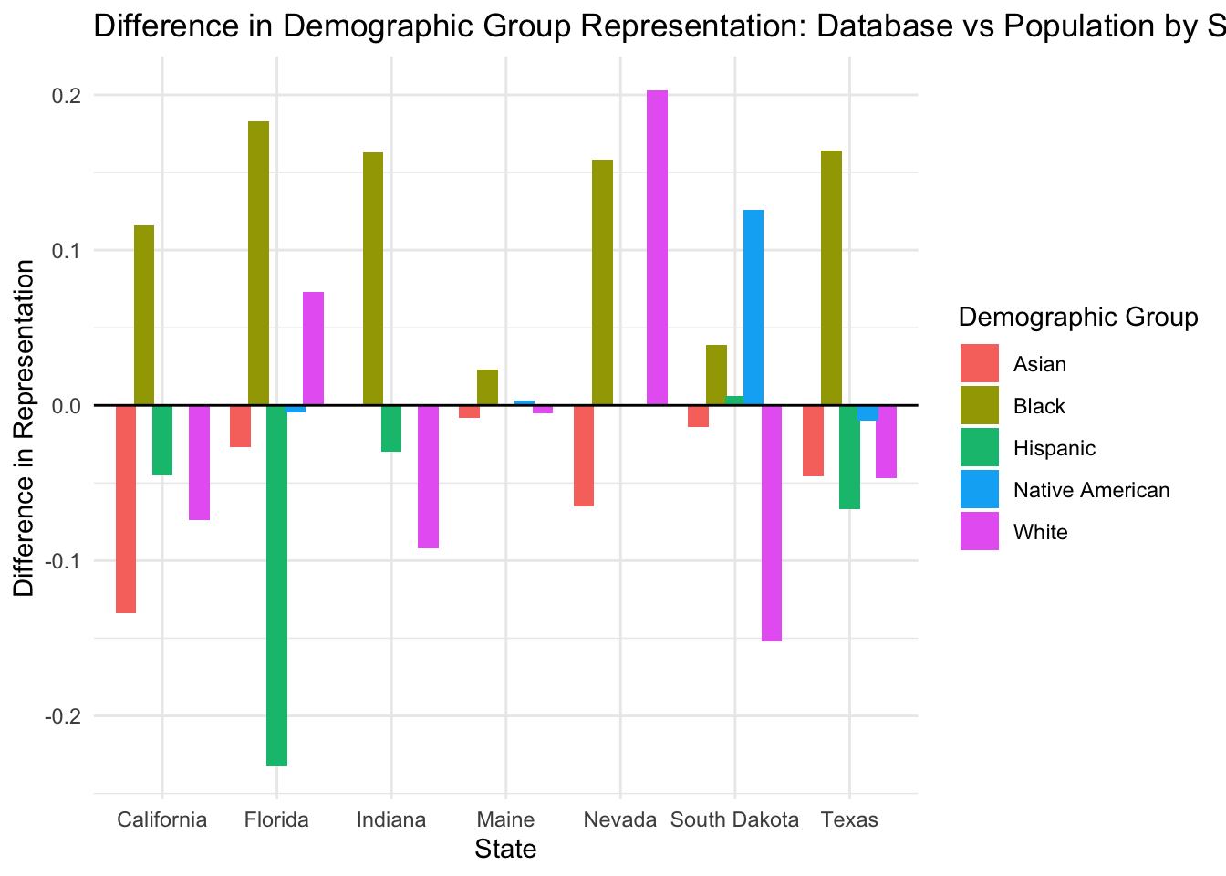
| Version | Author | Date |
|---|---|---|
| 9e71347 | Tina Lasisi | 2024-01-22 |
Summary Table
Finally, we create a summary table showing the difference in representation for each state and demographic group.
# Creating the summary table
state_group_summary <- merged_data %>%
  group_by(State, `Demographic Group`) %>%
  summarize(Difference = mean(Difference)) %>%
  ungroup()
`summarise()` has grouped output by 'State'. You can override using the
`.groups` argument.state_group_summary# A tibble: 35 × 3
State `Demographic Group` Difference
<chr> <chr> <dbl>
1 California Asian -0.134
2 California Black 0.116
3 California Hispanic -0.045
4 California Native American NA
5 California White -0.0740
6 Florida Asian -0.0267
7 Florida Black 0.183
8 Florida Hispanic -0.232
9 Florida Native American -0.0044
10 Florida White 0.0730
# ℹ 25 more rows
sessionInfo()R version 4.3.2 (2023-10-31)
Platform: aarch64-apple-darwin20 (64-bit)
Running under: macOS Sonoma 14.3.1
Matrix products: default
BLAS: /Library/Frameworks/R.framework/Versions/4.3-arm64/Resources/lib/libRblas.0.dylib
LAPACK: /Library/Frameworks/R.framework/Versions/4.3-arm64/Resources/lib/libRlapack.dylib; LAPACK version 3.11.0
locale:
[1] en_US.UTF-8/en_US.UTF-8/en_US.UTF-8/C/en_US.UTF-8/en_US.UTF-8
time zone: America/Detroit
tzcode source: internal
attached base packages:
[1] stats graphics grDevices utils datasets methods base
other attached packages:
[1] lubridate_1.9.3 forcats_1.0.0 stringr_1.5.1 dplyr_1.1.4
[5] purrr_1.0.2 readr_2.1.5 tidyr_1.3.0 tibble_3.2.1
[9] ggplot2_3.4.4 tidyverse_2.0.0 workflowr_1.7.1
loaded via a namespace (and not attached):
[1] sass_0.4.8 utf8_1.2.4 generics_0.1.3 stringi_1.8.3
[5] hms_1.1.3 digest_0.6.34 magrittr_2.0.3 timechange_0.2.0
[9] evaluate_0.23 grid_4.3.2 fastmap_1.1.1 rprojroot_2.0.4
[13] jsonlite_1.8.8 processx_3.8.3 whisker_0.4.1 ps_1.7.5
[17] promises_1.2.1 httr_1.4.7 fansi_1.0.6 scales_1.3.0
[21] jquerylib_0.1.4 cli_3.6.2 crayon_1.5.2 rlang_1.1.3
[25] bit64_4.0.5 munsell_0.5.0 withr_2.5.2 cachem_1.0.8
[29] yaml_2.3.8 parallel_4.3.2 tools_4.3.2 tzdb_0.4.0
[33] colorspace_2.1-0 httpuv_1.6.13 vctrs_0.6.5 R6_2.5.1
[37] lifecycle_1.0.4 git2r_0.33.0 bit_4.0.5 fs_1.6.3
[41] vroom_1.6.5 pkgconfig_2.0.3 callr_3.7.3 pillar_1.9.0
[45] bslib_0.6.1 later_1.3.2 gtable_0.3.4 glue_1.7.0
[49] Rcpp_1.0.12 highr_0.10 xfun_0.41 tidyselect_1.2.0
[53] rstudioapi_0.15.0 knitr_1.45 farver_2.1.1 htmltools_0.5.7
[57] labeling_0.4.3 rmarkdown_2.25 compiler_4.3.2 getPass_0.2-4