Short Range Familial Search
Tina Lasisi
2024-03-03 20:03:02
Last updated: 2024-03-03
Checks: 7 0
Knit directory: PODFRIDGE/
This reproducible R Markdown analysis was created with workflowr (version 1.7.1). The Checks tab describes the reproducibility checks that were applied when the results were created. The Past versions tab lists the development history.
Great! Since the R Markdown file has been committed to the Git repository, you know the exact version of the code that produced these results.
Great job! The global environment was empty. Objects defined in the global environment can affect the analysis in your R Markdown file in unknown ways. For reproduciblity it’s best to always run the code in an empty environment.
The command set.seed(20230302) was run prior to running
the code in the R Markdown file. Setting a seed ensures that any results
that rely on randomness, e.g. subsampling or permutations, are
reproducible.
Great job! Recording the operating system, R version, and package versions is critical for reproducibility.
Nice! There were no cached chunks for this analysis, so you can be confident that you successfully produced the results during this run.
Great job! Using relative paths to the files within your workflowr project makes it easier to run your code on other machines.
Great! You are using Git for version control. Tracking code development and connecting the code version to the results is critical for reproducibility.
The results in this page were generated with repository version 2596546. See the Past versions tab to see a history of the changes made to the R Markdown and HTML files.
Note that you need to be careful to ensure that all relevant files for
the analysis have been committed to Git prior to generating the results
(you can use wflow_publish or
wflow_git_commit). workflowr only checks the R Markdown
file, but you know if there are other scripts or data files that it
depends on. Below is the status of the Git repository when the results
were generated:
Ignored files:
    Ignored:    .DS_Store
    Ignored:    .Rhistory
    Ignored:    .Rproj.user/
    Ignored:    analysis/.DS_Store
    Ignored:    output/.DS_Store
Note that any generated files, e.g. HTML, png, CSS, etc., are not included in this status report because it is ok for generated content to have uncommitted changes.
These are the previous versions of the repository in which changes were
made to the R Markdown (analysis/STR.Rmd) and HTML
(docs/STR.html) files. If you’ve configured a remote Git
repository (see ?wflow_git_remote), click on the hyperlinks
in the table below to view the files as they were in that past version.
| File | Version | Author | Date | Message |
|---|---|---|---|---|
| Rmd | 2596546 | Tina Lasisi | 2024-03-03 | wflow_publish("analysis/*", republish = TRUE, all = TRUE, verbose = TRUE) |
| html | 2596546 | Tina Lasisi | 2024-03-03 | wflow_publish("analysis/*", republish = TRUE, all = TRUE, verbose = TRUE) |
| html | 48acb9f | Tina Lasisi | 2024-03-02 | Build site. |
| html | 5352065 | Tina Lasisi | 2024-03-02 | workflowr::wflow_publish(files = "analysis/*", all = TRUE, update = TRUE, |
| html | aa3ff5c | Tina Lasisi | 2024-03-01 | Build site. |
| Rmd | e4c698e | Tina Lasisi | 2024-02-27 | Publish new pages + update plots |
| html | e4c698e | Tina Lasisi | 2024-02-27 | Publish new pages + update plots |
| Rmd | acfb421 | Tina Lasisi | 2023-06-06 | Update simulation script |
| Rmd | d959019 | Tina Lasisi | 2023-05-31 | Add STR.Rmd |
CODIS marker allele frequencies
Frequencies and raw genotypes for different populations were found here and refer to Steffen, C.R., Coble, M.D., Gettings, K.B., Vallone, P.M. (2017) Corrigendum to ‘U.S. Population Data for 29 Autosomal STR Loci’ [Forensic Sci. Int. Genet. 7 (2013) e82-e83]. Forensic Sci. Int. Genet. 31, e36–e40. The US core CODIS markers are a subset of the 29 described here.
Load CODIS allele frequencies
CODIS allele frequencies were found through NIST STR base and specifically downloaded from the supplementary materials of Steffen et al 2017. These are 1036 unrelated individuals from the U.S. population.
# Define the file paths
file_paths <- list.files(path = "data", pattern = "1036_.*\\.csv", full.names = TRUE)

# Create a list of data frames
df_list <- lapply(file_paths, function(path) {
  read_csv(path, col_types = cols(
    marker = col_character(),
    allele = col_double(),
    frequency = col_double(),
    population = col_character()
  ))
})

# Bind all data frames into one
df <- bind_rows(df_list)

df_freq <- df
Simulating genotypes
Below, we assign probabilities to different familial relationships—parent-child, full siblings, half-siblings, cousins, second cousins, and unrelated—indicating the likelihood of sharing 0, 1, or 2 alleles identical by descent (IBD).
df_ibdprobs <- tibble(
  relationship =
    c("parent_child", "full_siblings", "half_siblings", "cousins", "second_cousins", "unrelated"),
  k0 = c(0, 1/4, 1/2, 7/8, 15/16, 1),
  k1 = c(1, 1/2, 1/2, 1/8, 1/16, 0),
  k2 = c(0, 1/4, 0, 0, 0, 0)
)

df_ibdprobs
# A tibble: 6 × 4
relationship k0 k1 k2
<chr> <dbl> <dbl> <dbl>
1 parent_child 0 1 0
2 full_siblings 0.25 0.5 0.25
3 half_siblings 0.5 0.5 0
4 cousins 0.875 0.125 0
5 second_cousins 0.938 0.0625 0
6 unrelated 1 0 0 simulate_STRpairs <- function(population, relationship_type, df_allelefreq, df_ibdprobs, n_sims=1) {
markers <- unique(df_allelefreq$marker)
allele_frequencies_by_marker <- df_allelefreq %>%
filter(population == population) %>%
split(.$marker)
allele_frequencies_by_marker <- map(allele_frequencies_by_marker, ~.x %>% pull(frequency) %>% setNames(.x$allele))
prob_shared_alleles <- df_ibdprobs %>%
filter(relationship == relationship) %>%
select(k0, k1, k2) %>%
unlist() %>%
as.numeric()
non_zero_indices <- which(prob_shared_alleles != 0)
k0 <- prob_shared_alleles[1]
k1 <- prob_shared_alleles[2]
k2 <- prob_shared_alleles[3]
results <- lapply(markers, function(current_marker) {
marker_results <- lapply(seq_len(n_sims), function(replicate_id) {
individual1 <- setNames(
lapply(markers, function(current_marker) {
allele_frequencies <- allele_frequencies_by_marker[[current_marker]]
return(sample(names(allele_frequencies), size = 2, replace = TRUE, prob = allele_frequencies))
}), markers)
individual2 <- setNames(
lapply(markers, function(current_marker) {
allele_frequencies <- allele_frequencies_by_marker[[current_marker]]
num_shared_alleles <- sample(non_zero_indices - 1, size = 1, prob = prob_shared_alleles[non_zero_indices])
alleles_from_individual1 <- sample(individual1[[current_marker]], size = num_shared_alleles)
alleles_from_population <- sample(names(allele_frequencies), size = 2 - num_shared_alleles, replace = TRUE, prob = allele_frequencies)
return(c(alleles_from_individual1, alleles_from_population))
}), markers)
ind1_alleles <- individual1[[current_marker]]
ind2_alleles <- individual2[[current_marker]]
shared_alleles <- intersect(ind1_alleles, ind2_alleles)
num_shared_alleles <- length(shared_alleles)
R_Xp <- sum(purrr::map_dbl(shared_alleles, function(x) unlist(allele_frequencies_by_marker[[current_marker]][x])))
R_Xu <- sum(purrr::map_dbl(ind1_alleles, function(x) unlist(allele_frequencies_by_marker[[current_marker]][x])) * purrr::map_dbl(ind2_alleles, function(x) unlist(allele_frequencies_by_marker[[current_marker]][x])))
R <- k0
if (R_Xp != 0) { R <- R + (k1 / R_Xp) }
if (R_Xu != 0) { R <- R + (k2 / R_Xu) }
log_R <- log(R)
# Add the replicate_id column to the output tibble
return(tibble(population = population,
relationship_type = relationship_type,
marker = current_marker,
num_shared_alleles = num_shared_alleles,
log_R = log_R,
replicate_id = replicate_id)) # Add this line
})
marker_results <- bind_rows(marker_results)
return(marker_results)
})
result <- bind_rows(results)
# Aggregate results for each replicate, summing num_shared_alleles and log_R values.
result_by_replicate <- result %>%
group_by(population, relationship_type, replicate_id) %>%
summarise(num_shared_alleles_sum = sum(num_shared_alleles),
log_R_sum = sum(log_R),
.groups = "drop")
return(result_by_replicate)
}Combinations
simulation_combinations <- function(df, n_sims_unrelated, n_sims_related) {
  # Define the list of relationship types
  relationship_types <- c('parent_child', 'full_siblings', 'half_siblings', 'cousins', 'second_cousins', 'unrelated')

  # Get unique populations from the input dataframe
  unique_populations <- unique(df$population)
  filtered_populations <- unique_populations[unique_populations != "all"]

  # Create a dataframe of all combinations of populations and relationship types
  combinations <- expand_grid(population = filtered_populations, relationship_type = relationship_types)

  # Add the number of simulations for unrelated or related relationships
  combinations$n_sims <- ifelse(combinations$relationship_type == "unrelated", n_sims_unrelated, n_sims_related)

  return(combinations)
}
# Example usage
result_combinations <- simulation_combinations(df, n_sims_unrelated = 10, n_sims_related = 5)
result_combinations# A tibble: 24 × 3
population relationship_type n_sims
<chr> <chr> <dbl>
1 AfAm parent_child 5
2 AfAm full_siblings 5
3 AfAm half_siblings 5
4 AfAm cousins 5
5 AfAm second_cousins 5
6 AfAm unrelated 10
7 Asian parent_child 5
8 Asian full_siblings 5
9 Asian half_siblings 5
10 Asian cousins 5
# ℹ 14 more rowsParallel
# # Apply the simulate_STRpairs function to each row in result_combinations
# results <- result_combinations %>%
#   pmap_dfr(function(population, relationship_type, n_sims) {
#     simulate_STRpairs(population, relationship_type, df_allelefreq = df_freq, df_ibdprobs = df_ibdprobs, n_sims = n_sims)
#   })
Figures
# Function to capitalize the first letter of a string
ucfirst <- function(s) {
  paste(toupper(substring(s, 1,1)), substring(s, 2), sep = "")
}

create_plot <- function(df, variable_to_plot, relationship_col, population_col) {
  # Set the population_shape variable as factor
  df$population_shape <- factor(df[[population_col]])

  # Create the plot
  p <- ggplot(df, aes(x = .data[[relationship_col]], y = .data[[variable_to_plot]],
                      color = .data[[population_col]], shape = .data[[population_col]], fill = .data[[population_col]])) +
    geom_boxplot(alpha = 0.4, position = position_dodge(width = 0.75)) +
    geom_point(position = position_jitterdodge(jitter.width = 0.1, dodge.width = 0.75), size = 1, alpha = 0.6) +
    theme_classic() +
    theme(axis.text.x = element_text(angle = 45, hjust = 1)) +
    scale_x_discrete(limits = c('parent_child', 'full_siblings', 'half_siblings', 'cousins', 'second_cousins', 'unrelated')) +
    scale_shape_manual(values = c(16, 17, 15, 18)) + # Change these values to desired shapes
    labs(title = paste(ucfirst(variable_to_plot), "by Relationship Type and Population"),
         x = "Relationship Type",
         y = ucfirst(variable_to_plot),
         color = "Population",
         shape = "Population",
         fill = "Population")

  # Save the plot to the /output folder with a custom file name
  save_plot <- function(plot, plot_name) {
    ggsave(filename = paste0("output/", plot_name, ".png"), plot = plot, height = 6, width = 8, units = "in")
  }

  # Call the save_plot function to save the plot
  save_plot(p, paste("plot_", variable_to_plot, sep = ""))

  return(p)
}
simulation_results <- read.csv("data/simulation_results.csv")# Filter your data for unique STR markers and remove the "all" population
# df_plt_final <- results_parallel %>%
df_plt_final <- simulation_results %>%
select(-replicate_id)
p <- create_plot(df_plt_final, "log_R_sum", "relationship_type", "population")
p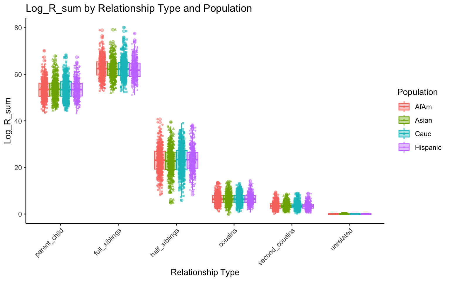
| Version | Author | Date |
|---|---|---|
| e4c698e | Tina Lasisi | 2024-02-27 |
plt_allele <- create_plot(df_plt_final, "num_shared_alleles_sum", "relationship_type", "population")
plt_allele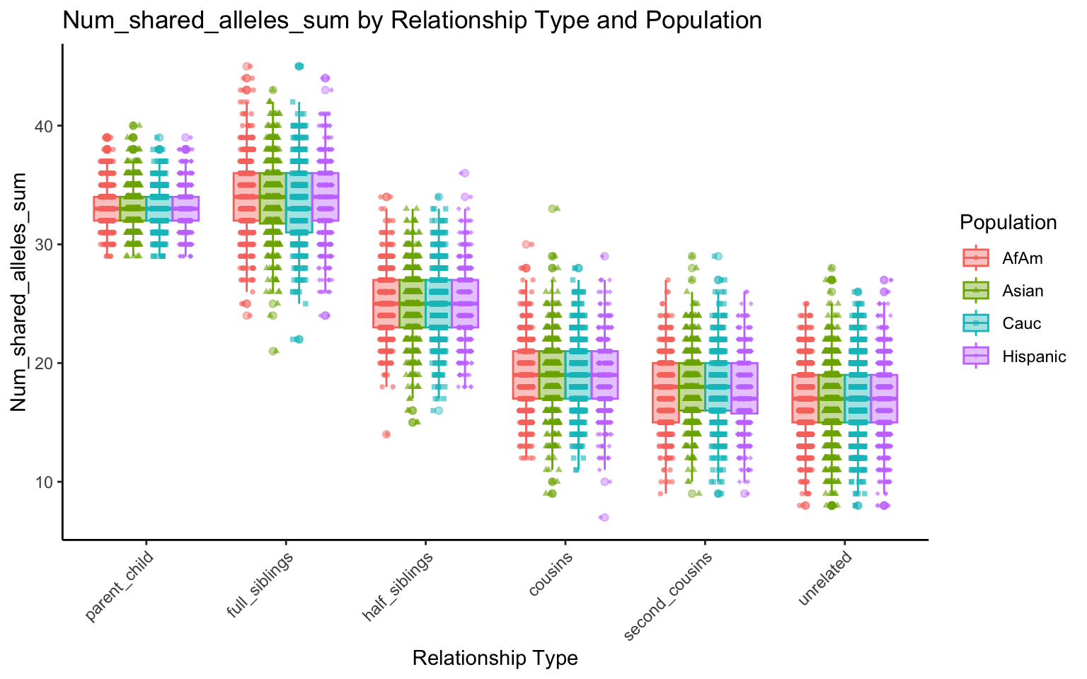
| Version | Author | Date |
|---|---|---|
| e4c698e | Tina Lasisi | 2024-02-27 |
sessionInfo()R version 4.3.2 (2023-10-31)
Platform: aarch64-apple-darwin20 (64-bit)
Running under: macOS Sonoma 14.3.1
Matrix products: default
BLAS: /Library/Frameworks/R.framework/Versions/4.3-arm64/Resources/lib/libRblas.0.dylib
LAPACK: /Library/Frameworks/R.framework/Versions/4.3-arm64/Resources/lib/libRlapack.dylib; LAPACK version 3.11.0
locale:
[1] en_US.UTF-8/en_US.UTF-8/en_US.UTF-8/C/en_US.UTF-8/en_US.UTF-8
time zone: America/Detroit
tzcode source: internal
attached base packages:
[1] stats graphics grDevices utils datasets methods base
other attached packages:
[1] progressr_0.14.0 furrr_0.3.1 future_1.33.1 lubridate_1.9.3
[5] forcats_1.0.0 stringr_1.5.1 dplyr_1.1.4 purrr_1.0.2
[9] readr_2.1.5 tidyr_1.3.0 tibble_3.2.1 ggplot2_3.4.4
[13] tidyverse_2.0.0 readxl_1.4.3 workflowr_1.7.1
loaded via a namespace (and not attached):
[1] gtable_0.3.4 xfun_0.41 bslib_0.6.1 processx_3.8.3
[5] callr_3.7.3 tzdb_0.4.0 vctrs_0.6.5 tools_4.3.2
[9] ps_1.7.5 generics_0.1.3 parallel_4.3.2 fansi_1.0.6
[13] highr_0.10 pkgconfig_2.0.3 lifecycle_1.0.4 farver_2.1.1
[17] compiler_4.3.2 git2r_0.33.0 textshaping_0.3.7 munsell_0.5.0
[21] getPass_0.2-4 codetools_0.2-19 httpuv_1.6.13 htmltools_0.5.7
[25] sass_0.4.8 yaml_2.3.8 crayon_1.5.2 later_1.3.2
[29] pillar_1.9.0 jquerylib_0.1.4 whisker_0.4.1 cachem_1.0.8
[33] parallelly_1.36.0 tidyselect_1.2.0 digest_0.6.34 stringi_1.8.3
[37] listenv_0.9.0 labeling_0.4.3 rprojroot_2.0.4 fastmap_1.1.1
[41] grid_4.3.2 colorspace_2.1-0 cli_3.6.2 magrittr_2.0.3
[45] utf8_1.2.4 withr_2.5.2 scales_1.3.0 promises_1.2.1
[49] bit64_4.0.5 timechange_0.2.0 rmarkdown_2.25 httr_1.4.7
[53] globals_0.16.2 bit_4.0.5 cellranger_1.1.0 ragg_1.2.7
[57] hms_1.1.3 evaluate_0.23 knitr_1.45 rlang_1.1.3
[61] Rcpp_1.0.12 glue_1.7.0 vroom_1.6.5 rstudioapi_0.15.0
[65] jsonlite_1.8.8 R6_2.5.1 systemfonts_1.0.5 fs_1.6.3