PCA

workflowr

• Summary
• Checks
• Past versions

Last updated: 2025-02-04

Checks: 6 1

Knit directory: sapphire/

This reproducible R Markdown analysis was created with workflowr (version 1.7.1). The Checks tab describes the reproducibility checks that were applied when the results were created. The Past versions tab lists the development history.

---

R Markdown file: up-to-date

Great! Since the R Markdown file has been committed to the Git repository, you know the exact version of the code that produced these results.

Environment: empty

Great job! The global environment was empty. Objects defined in the global environment can affect the analysis in your R Markdown file in unknown ways. For reproduciblity it’s best to always run the code in an empty environment.

Seed: set.seed(20240923)

The command set.seed(20240923) was run prior to running the code in the R Markdown file. Setting a seed ensures that any results that rely on randomness, e.g. subsampling or permutations, are reproducible.

Session information: recorded

Great job! Recording the operating system, R version, and package versions is critical for reproducibility.

Cache: none

Nice! There were no cached chunks for this analysis, so you can be confident that you successfully produced the results during this run.

File paths: absolute

Using absolute paths to the files within your workflowr project makes it difficult for you and others to run your code on a different machine. Change the absolute path(s) below to the suggested relative path(s) to make your code more reproducible.

absolute	relative
~/sapphire/data/serum_vit_D_study_with_lab_results.xlsx	data/serum_vit_D_study_with_lab_results.xlsx
~/sapphire/data/sun_expos_data/sun_expos_long.csv	data/sun_expos_data/sun_expos_long.csv

Repository version: 564ea55

Great! You are using Git for version control. Tracking code development and connecting the code version to the results is critical for reproducibility.

The results in this page were generated with repository version 564ea55. See the Past versions tab to see a history of the changes made to the R Markdown and HTML files.

Note that you need to be careful to ensure that all relevant files for the analysis have been committed to Git prior to generating the results (you can use wflow_publish or wflow_git_commit). workflowr only checks the R Markdown file, but you know if there are other scripts or data files that it depends on. Below is the status of the Git repository when the results were generated:

Ignored files:
    Ignored:    .DS_Store
    Ignored:    .RData
    Ignored:    .Rhistory
    Ignored:    .Rproj.user/
    Ignored:    analysis/.RData
    Ignored:    analysis/.Rhistory

Untracked files:
    Untracked:  .lock_gPLINK
    Untracked:  .metafile_gPLINK
    Untracked:  SAfrADMIX/
    Untracked:  analysis/genotype.R
    Untracked:  analysis/lilyanalysis.Rmd
    Untracked:  data/dist_pops.csv
    Untracked:  data/summer_winter.csv

Note that any generated files, e.g. HTML, png, CSS, etc., are not included in this status report because it is ok for generated content to have uncommitted changes.

---

These are the previous versions of the repository in which changes were made to the R Markdown (analysis/pca.Rmd) and HTML (docs/pca.html) files. If you’ve configured a remote Git repository (see ?wflow_git_remote), click on the hyperlinks in the table below to view the files as they were in that past version.

File	Version	Author	Date	Message
html	564ea55	Lily Heald	2025-02-04	Build site.
Rmd	d9fb6da	Lily Heald	2025-02-04	wflow
html	d9fb6da	Lily Heald	2025-02-04	wflow
Rmd	517cf8d	Lily Heald	2025-02-04	More analyses
Rmd	131b1d2	Lily Heald	2025-01-22	initial PCAs

---

file_path <- "~/sapphire/data/serum_vit_D_study_with_lab_results.xlsx" 
data_summer <- read_excel(file_path, sheet = "ScreeningDataCollectionSummer")
data_winter <- read_excel(file_path, sheet = "ScreeningDataCollectionWinter")
data_6weeks <- read_excel(file_path, sheet = "ScreeningDataCollection6Weeks")
sun_expos <- read.csv("~/sapphire/data/sun_expos_data/sun_expos_long.csv")
sun_expos_summer <- sun_expos[sun_expos$collection_period == 'Summer', ]
sun_expos_winter <- sun_expos[sun_expos$collection_period == 'Winter', ]
sun_expos_6Weeks <- sun_expos[sun_expos$collection_period == '6Weeks', ]

part 0: cleaning

summer_data <- left_join(data_summer, sun_expos_summer,
                     by = c("ParticipantCentreID" = "participant_centre_id"))

winter_data <- left_join(data_winter, sun_expos_winter,
                     by = c("ParticipantCentreID" = "participant_centre_id"))

six_week_data <- left_join(data_6weeks, sun_expos_6Weeks,
                     by = c("ParticipantCentreID" = "participant_centre_id"))

summer_data = subset(summer_data, select = -c(Supplements, Medications,
                                              EthnicitySpecifyOther, SmokingComments,
                                              x9if_apply_sunscreen_spf_used))
winter_data = subset(winter_data, select = -c(Supplements, Medications,
                                              EthnicitySpecifyOther, SmokingComments,
                                              ContinuedInStudy, IfNotContinuedInStudyReason,
                                              x9if_apply_sunscreen_spf_used))
six_week_data = subset(six_week_data, select = -c(Supplements, Medications,
                                              EthnicitySpecifyOther, SmokingComments,
                                              ContinuedInStudy, IfNotContinuedInStudyReason,
                                              x9if_apply_sunscreen_spf_used))
six_week_data = six_week_data[,!grepl("IfNoReasonForExclusion:",names(six_week_data))]
winter_data = winter_data[,!grepl("IfNoReasonForExclusion:",names(winter_data))]
summer_data = summer_data[,!grepl("IfNoReasonForExclusion:",names(summer_data))]
six_week_data = six_week_data[,!grepl("Req Num",names(six_week_data))]
winter_data = winter_data[,!grepl("Req Num",names(winter_data))]
summer_data = summer_data[,!grepl("Req Num",names(summer_data))]
six_week_data <- data_6weeks
summer_data <- data_summer
winter_data <- data_winter

# taking the median of three measurements
sites <- c("Forehead", "RightUpperInnerArm", "LeftUpperInnerArm")
metrics <- c("E", "M", "R", "G", "B", "L\\*", "a\\*", "b\\*")
seasons <- c("six_week_data", "summer_data", "winter_data")

for(site in sites) {
  for(metric in metrics) {
    six_week_data <- six_week_data %>%
      rowwise() %>%
      mutate(!!paste0("Median", site, metric) := median(c_across(matches(paste0("SkinReflectance", site, metric, "[123]"))), na.rm = TRUE)) %>%
      ungroup()
  }
}

for(site in sites) {
  for(metric in metrics) {
    summer_data <- summer_data %>%
      rowwise() %>%
      mutate(!!paste0("Median", site, metric) := median(c_across(matches(paste0("SkinReflectance", site, metric, "[123]"))), na.rm = TRUE)) %>%
      ungroup()
  }
}

for(site in sites) {
  for(metric in metrics) {
    winter_data <- winter_data %>%
      rowwise() %>%
      mutate(!!paste0("Median", site, metric) := median(c_across(matches(paste0("SkinReflectance", site, metric, "[123]"))), na.rm = TRUE)) %>%
      ungroup()
  }
}

winter_data <- winter_data %>%
  select(-matches(".*[EMRGBL\\*a\\*b\\*]\\d$"))

summer_data <- summer_data %>%
  select(-matches(".*[EMRGBL\\*a\\*b\\*]\\d$"))

six_week_data <- six_week_data %>%
  select(-matches(".*[EMRGBL\\*a\\*b\\*]\\d$"))

ethnicity <- function(EthnicityAfricanBlack, EthnicityColoured, EthnicityWhite, 
                      EthnicityIndianAsian) {
  case_when(
    EthnicityAfricanBlack == TRUE & 
      EthnicityColoured == FALSE & 
      EthnicityWhite == FALSE & 
      EthnicityIndianAsian == FALSE ~ "Xhosa",
    EthnicityAfricanBlack == FALSE & 
      EthnicityColoured == TRUE & 
      EthnicityWhite == FALSE & 
      EthnicityIndianAsian == FALSE ~ "Cape_colored",
    TRUE ~ NA_character_
  )
}

summer_data <- summer_data %>%
  mutate(Ethnicity = ethnicity(EthnicityAfricanBlack, EthnicityColoured, 
                               EthnicityWhite, EthnicityIndianAsian))
summer_data = subset(summer_data, select = -c(EthnicityAfricanBlack, 
                                               EthnicityColoured, EthnicityWhite, 
                                               EthnicityIndianAsian))

winter_data <- winter_data %>%
  mutate(Ethnicity = ethnicity(EthnicityAfricanBlack, EthnicityColoured, 
                               EthnicityWhite, EthnicityIndianAsian))
winter_data = subset(winter_data, select = -c(EthnicityAfricanBlack, 
                                               EthnicityColoured, EthnicityWhite, 
                                               EthnicityIndianAsian))

six_week_data <- six_week_data %>%
  mutate(Ethnicity = ethnicity(EthnicityAfricanBlack, EthnicityColoured, 
                               EthnicityWhite, EthnicityIndianAsian))
six_week_data = subset(six_week_data, select = -c(EthnicityAfricanBlack, 
                                               EthnicityColoured, EthnicityWhite, 
                                               EthnicityIndianAsian))

ggplot(six_week_data, aes(x = VitDResult, y = MedianForeheadM, color = Ethnicity)) +
  geom_jitter() +
  theme(legend.position = "right")

Warning: Removed 1 row containing missing values or values outside the scale range
(`geom_point()`).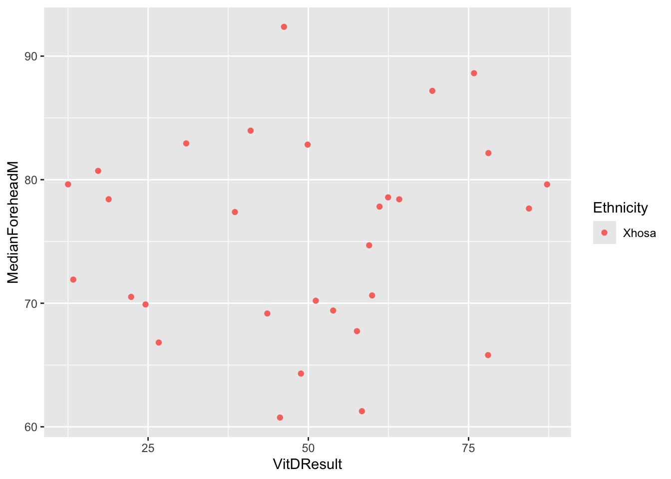

Past versions of dist_initial-1.png

Version	Author	Date
d9fb6da	Lily Heald	2025-02-04

ggplot(six_week_data, aes(x = Ethnicity, y = MedianForeheadM, color = Ethnicity, fill = Ethnicity)) + 
  geom_violin()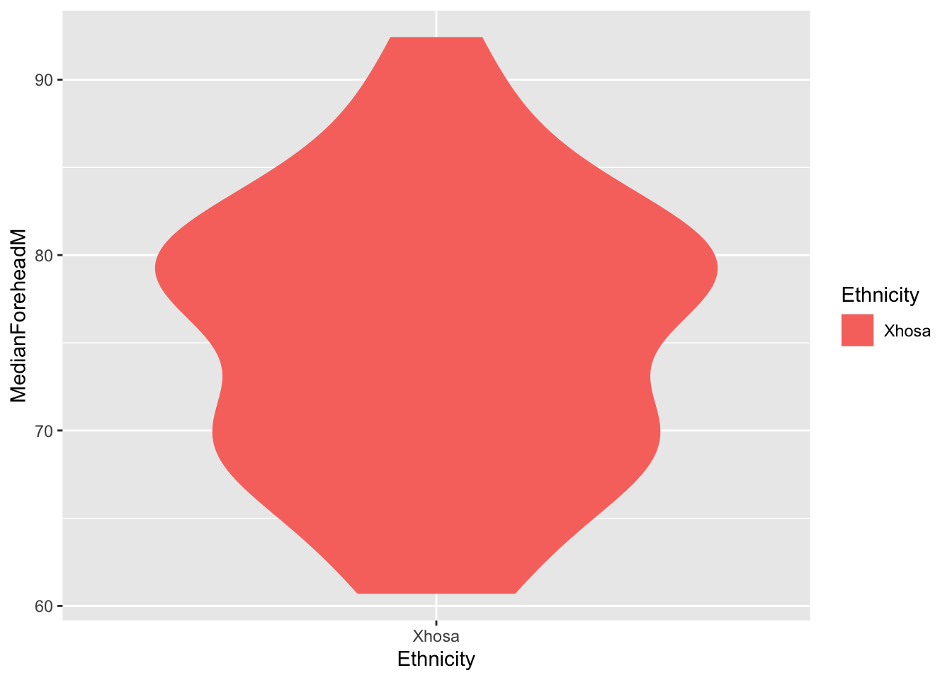

Past versions of dist_initial-2.png

Version	Author	Date
d9fb6da	Lily Heald	2025-02-04

ggplot(summer_data, aes(x = VitDResult, y = MedianForeheadM, color = Ethnicity)) +
  geom_jitter() +
  theme(legend.position = "right")

Warning: Removed 1 row containing missing values or values outside the scale range
(`geom_point()`).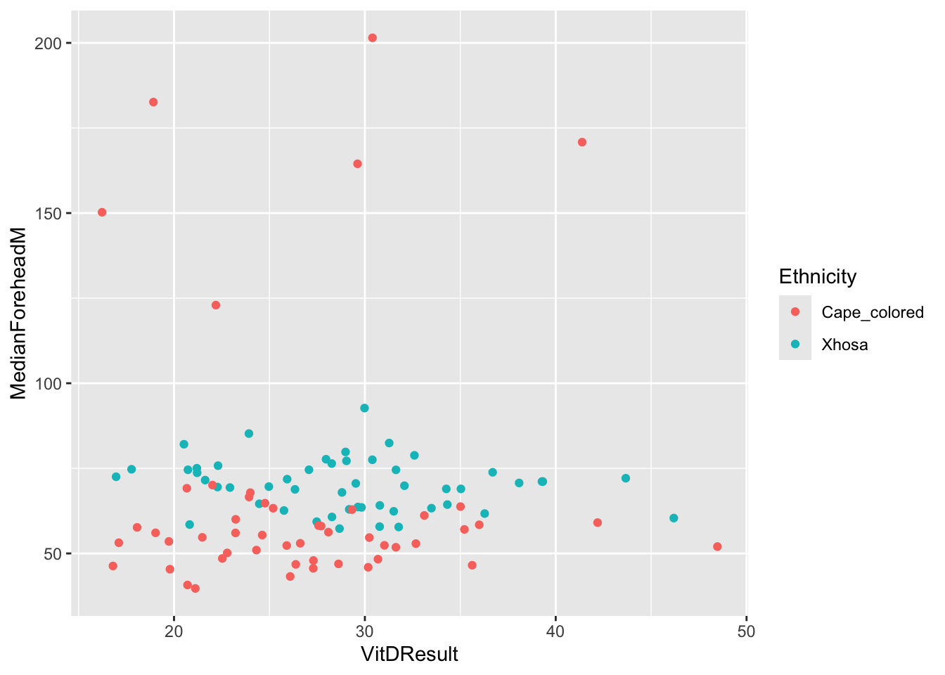

Past versions of dist_initial-3.png

Version	Author	Date
d9fb6da	Lily Heald	2025-02-04

ggplot(summer_data, aes(x = Ethnicity, y = MedianForeheadM, color = Ethnicity, fill = Ethnicity)) + 
  geom_boxplot()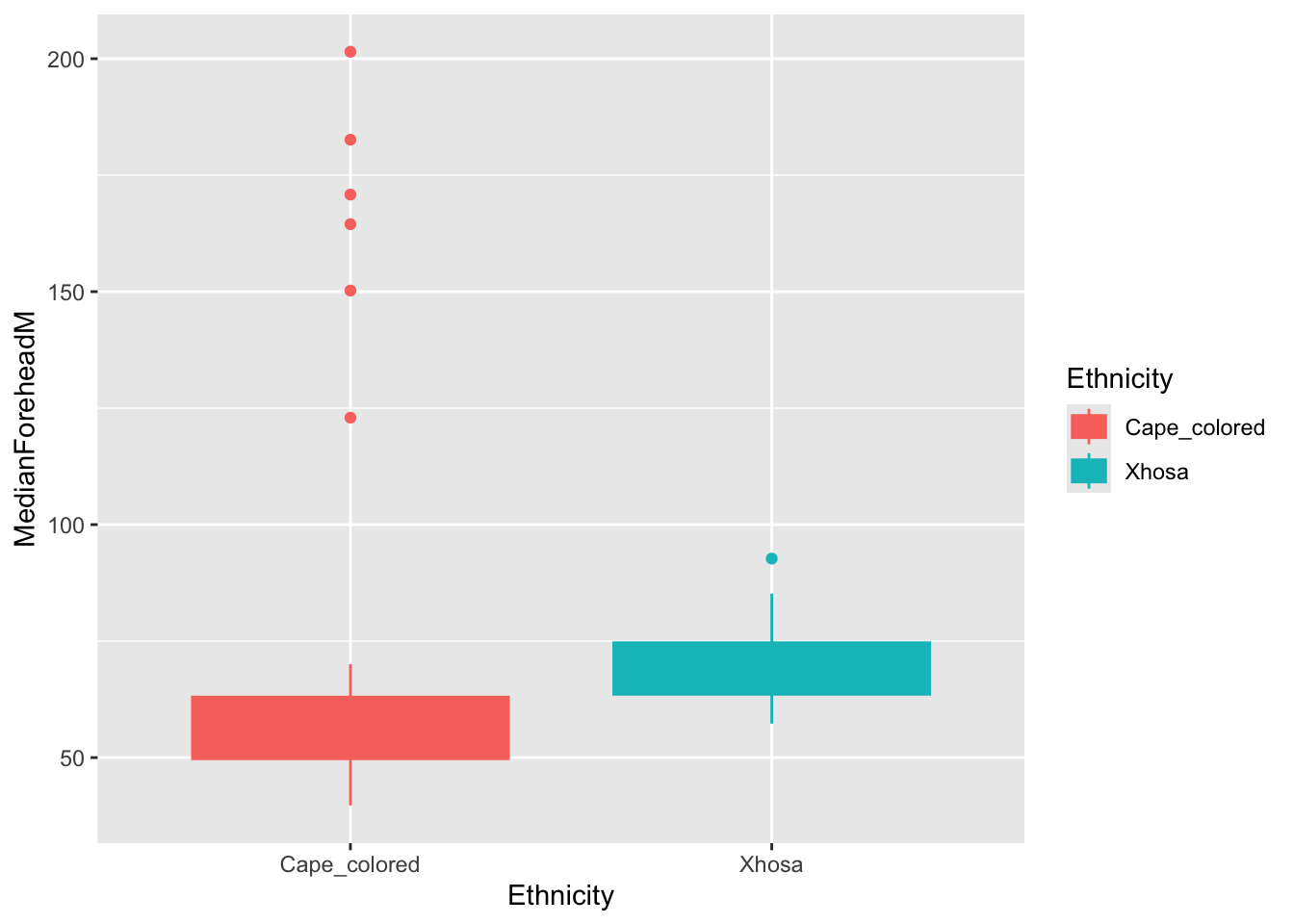

Past versions of dist_initial-4.png

Version	Author	Date
d9fb6da	Lily Heald	2025-02-04

# there are still outliers even when taking the median
for(site in sites) {
  for(metric in metrics) {
    column_name <- paste0("Median", site, metric)
    iqr <- IQR(winter_data[[column_name]], na.rm = TRUE)
    Q <- quantile(winter_data[[column_name]], probs = c(0.25, 0.75), na.rm = TRUE)
    up <- Q[2] + 1.5 * iqr
    low <- Q[1] - 1.5 * iqr
    winter_data <- winter_data %>%
      filter(!!sym(column_name) > low & !!sym(column_name) < up)
  }
}

for(site in sites) {
  for(metric in metrics) {
    column_name <- paste0("Median", site, metric)
    iqr <- IQR(summer_data[[column_name]], na.rm = TRUE)
    Q <- quantile(summer_data[[column_name]], probs = c(0.25, 0.75), na.rm = TRUE)
    up <- Q[2] + 1.5 * iqr
    low <- Q[1] - 1.5 * iqr
    summer_data <- summer_data %>%
      filter(!!sym(column_name) > low & !!sym(column_name) < up)
  }
}

for(site in sites) {
  for(metric in metrics) {
    column_name <- paste0("Median", site, metric)
    iqr <- IQR(winter_data[[column_name]], na.rm = TRUE)
    Q <- quantile(winter_data[[column_name]], probs = c(0.25, 0.75), na.rm = TRUE)
    up <- Q[2] + 1.5 * iqr
    low <- Q[1] - 1.5 * iqr
    six_week_data <- six_week_data %>%
      filter(!!sym(column_name) > low & !!sym(column_name) < up)
  }
}

ggplot(six_week_data, aes(x = VitDResult, y = MedianForeheadM, color = Ethnicity)) +
  geom_jitter() +
  theme(legend.position = "right")

Warning: Removed 1 row containing missing values or values outside the scale range
(`geom_point()`).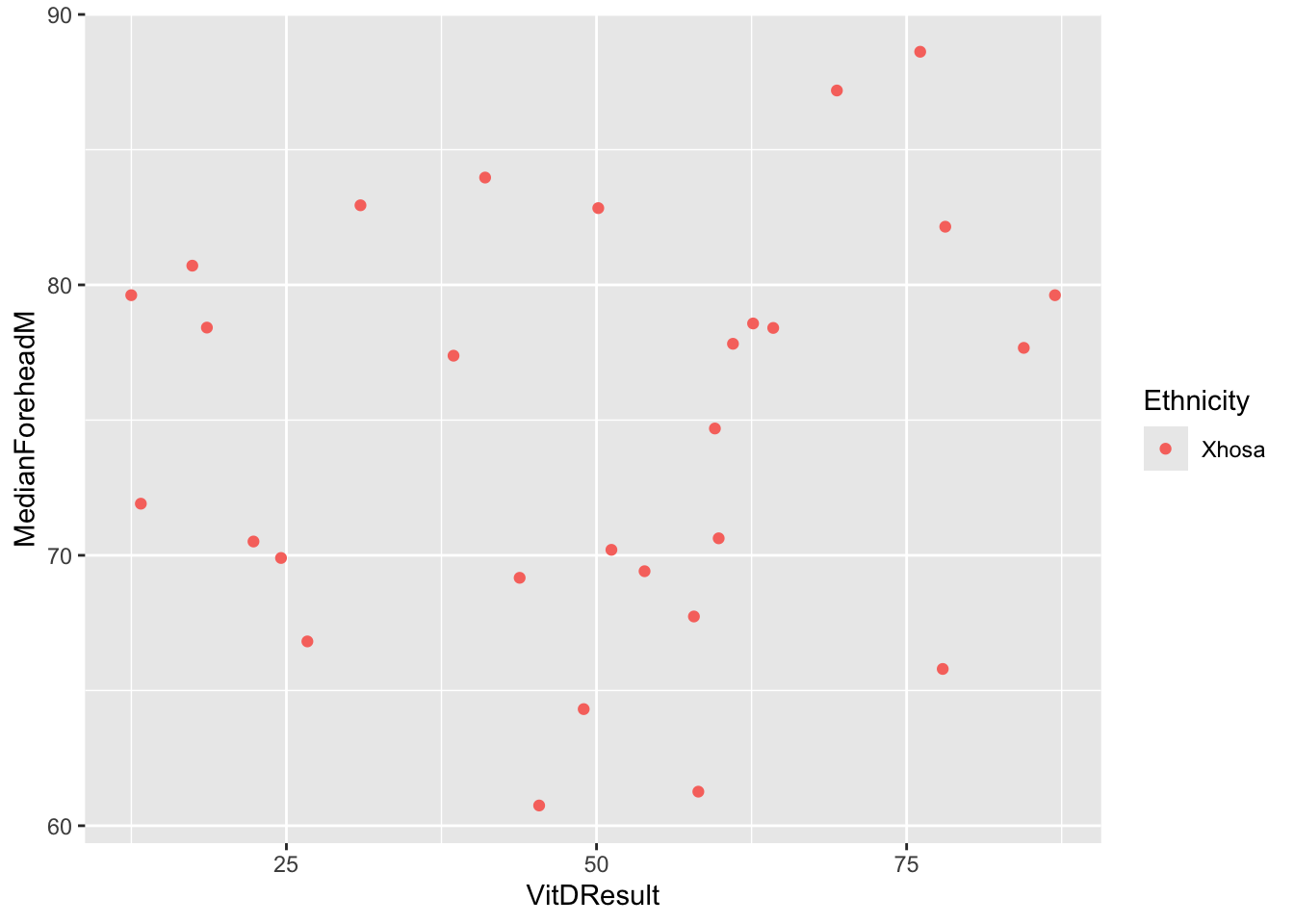

Past versions of dist_trimmed-1.png

Version	Author	Date
d9fb6da	Lily Heald	2025-02-04

ggplot(six_week_data, aes(x = Ethnicity, y = MedianForeheadM, color = Ethnicity, fill = Ethnicity)) + 
  geom_violin()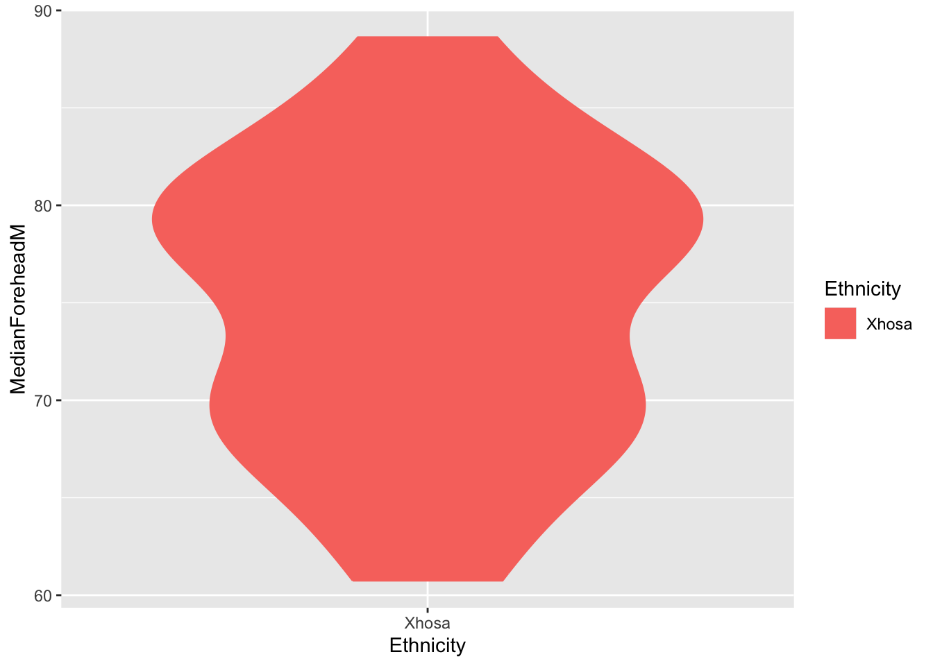

Past versions of dist_trimmed-2.png

Version	Author	Date
d9fb6da	Lily Heald	2025-02-04

ggplot(summer_data, aes(x = VitDResult, y = MedianForeheadM, color = Ethnicity)) +
  geom_jitter() +
  theme(legend.position = "right")

Warning: Removed 1 row containing missing values or values outside the scale range
(`geom_point()`).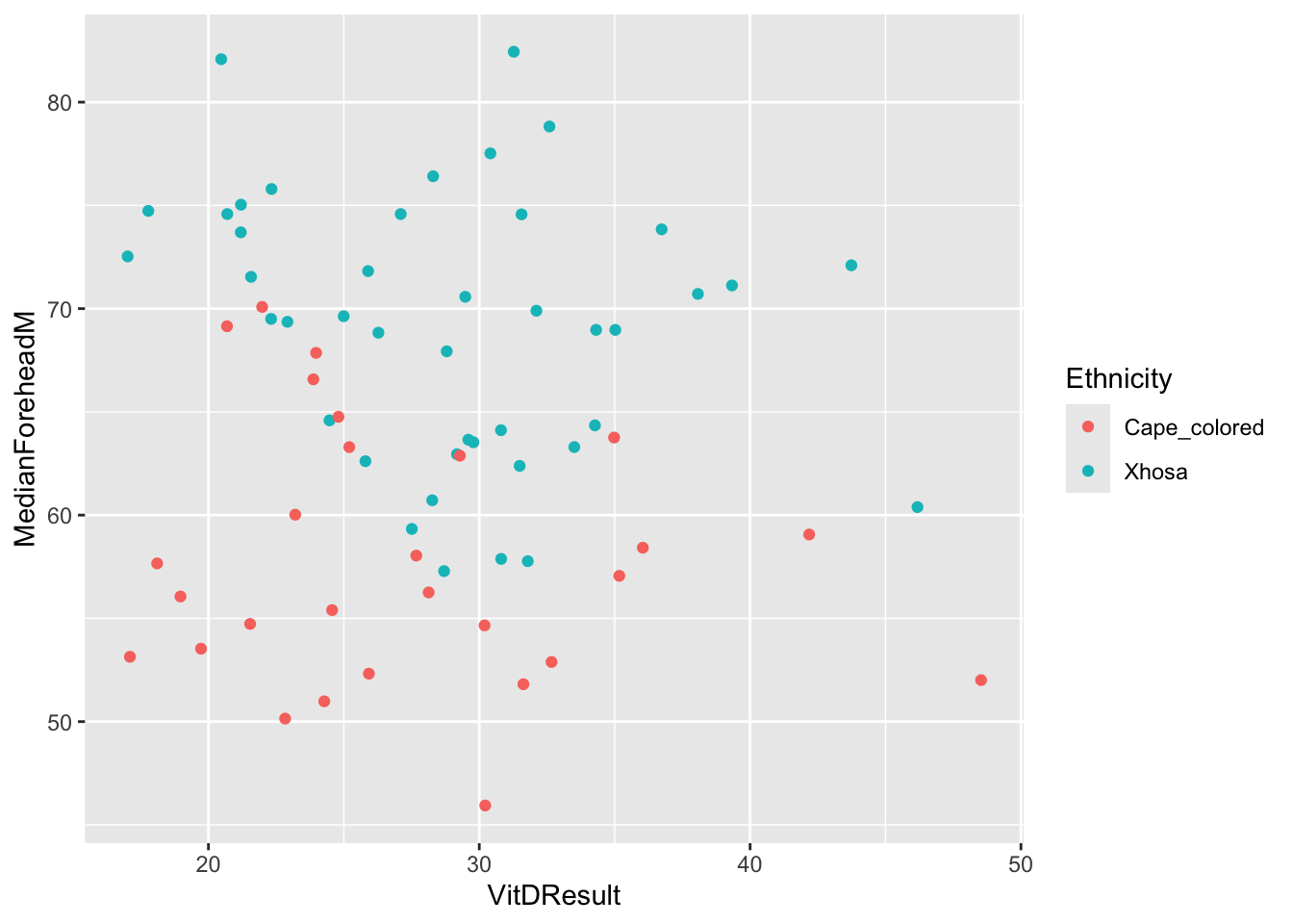

Past versions of dist_trimmed-3.png

Version	Author	Date
d9fb6da	Lily Heald	2025-02-04

ggplot(summer_data, aes(x = Ethnicity, y = MedianForeheadM, color = Ethnicity, fill = Ethnicity)) + 
  geom_boxplot()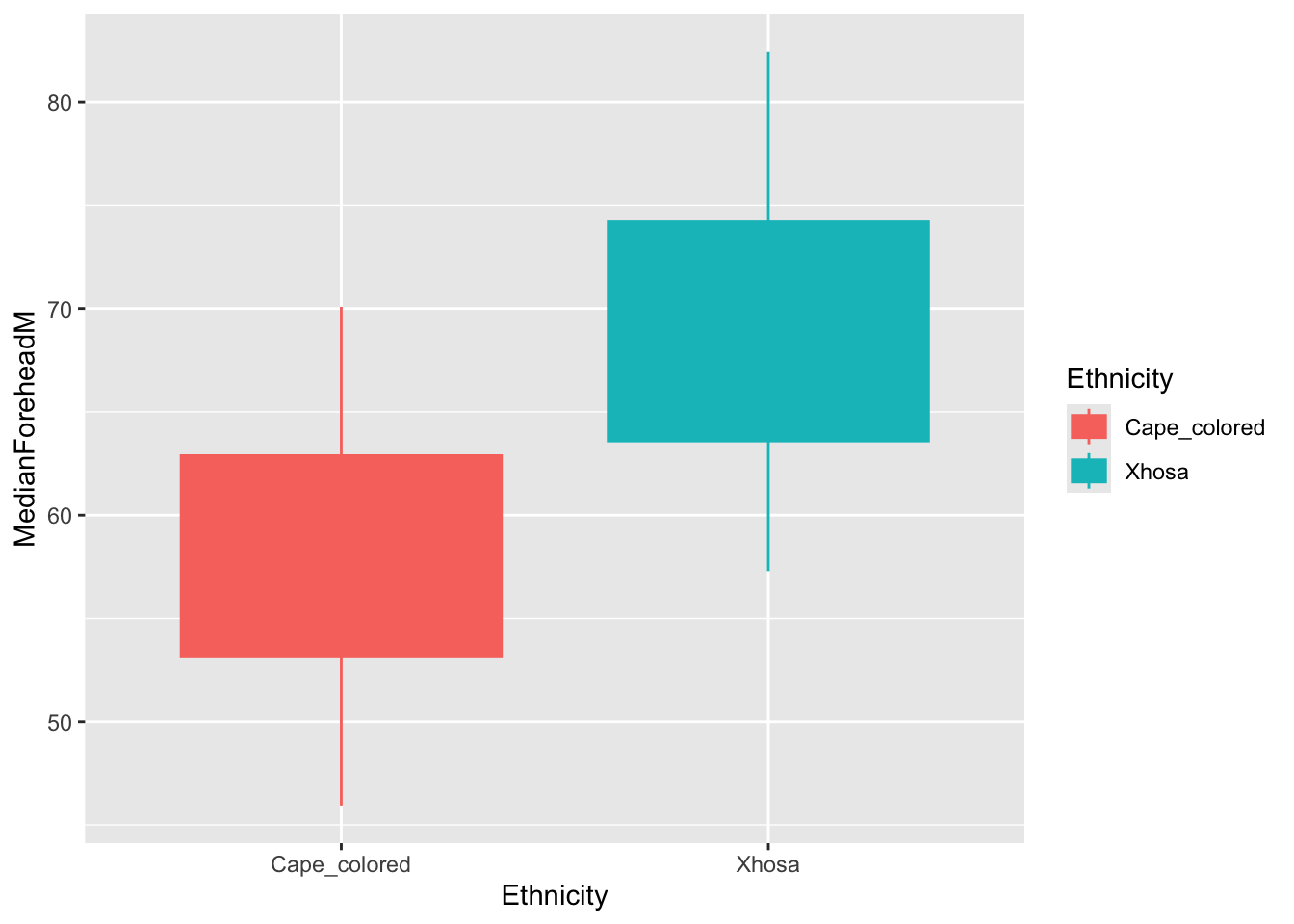

Past versions of dist_trimmed-4.png

Version	Author	Date
d9fb6da	Lily Heald	2025-02-04

# mean left and right inner arm
for (metric in metrics) {
  summer_data <- summer_data %>%
    mutate(!!paste0("InnerArm", metric) := rowMeans(
      select(., starts_with(paste0("MedianLeftInnerArm", metric)),
                 starts_with(paste0("MedianRightUpperInnerArm", metric))),
      na.rm = TRUE
    ))
}

for (metric in metrics) {
  winter_data <- winter_data %>%
    mutate(!!paste0("InnerArm", metric) := rowMeans(
      select(., starts_with(paste0("MedianLeftInnerArm", metric)),
                 starts_with(paste0("MedianRightUpperInnerArm", metric))),
      na.rm = TRUE
    ))
}

for (metric in metrics) {
  six_week_data <- six_week_data %>%
    mutate(!!paste0("InnerArm", metric) := rowMeans(
      select(., starts_with(paste0("MedianLeftInnerArm", metric)),
                 starts_with(paste0("MedianRightUpperInnerArm", metric))),
      na.rm = TRUE
    ))
}

winter_data <- winter_data %>%
  select(-matches("Left|Right"))

summer_data <- summer_data %>%
  select(-matches("Left|Right"))

six_week_data <- six_week_data %>%
  select(-matches("Left|Right"))

for (metric in metrics) {
  six_week_data <- six_week_data %>%
    mutate(!!paste0(metric, "Difference") :=
             .[[paste0("MedianForehead", metric)]] -
             .[[paste0("InnerArm", metric)]])
}

for (metric in metrics) {
  summer_data <- summer_data %>%
    mutate(!!paste0(metric, "Difference") :=
             .[[paste0("MedianForehead", metric)]] -
             .[[paste0("InnerArm", metric)]])
}

for (metric in metrics) {
  winter_data <- winter_data %>%
    mutate(!!paste0(metric, "Difference") :=
             .[[paste0("MedianForehead", metric)]] -
             .[[paste0("InnerArm", metric)]])
}

six_week_rename <- six_week_data %>%
    rename_with(~ paste0(., "_sixweeks"), -ParticipantCentreID)

joinone <- left_join(summer_data, winter_data, 
                     by = "ParticipantCentreID", 
                     suffix = c("_summer", "_winter"))

joined_data <- left_join(joinone, six_week_rename, 
                         by = "ParticipantCentreID")

head(joined_data)

# A tibble: 6 × 197
  ParticipantCentreID InterviewerName_summer TodayDate_summer    AgeYears_summer
  <chr>               <chr>                  <dttm>                        <dbl>
1 VDKH001             Betty                  2013-02-11 00:00:00              20
2 VDKH002             Betty                  2013-02-11 00:00:00              23
3 VDKH003             Betty                  2013-02-11 00:00:00              23
4 VDKH005             Betty                  2013-02-12 00:00:00              19
5 VDKH006             Betty                  2013-02-12 00:00:00              21
6 VDKH007             Betty                  2013-02-12 00:00:00              22
# ℹ 193 more variables: DateOfBirth_summer <dttm>, Gender_summer <dbl>,
#   EthnicityOther_summer <lgl>, EthnicitySpecifyOther_summer <lgl>,
#   Ethnicity_summer <chr>, RefuseToAnswer_summer <lgl>,
#   AvgWeight_summer <dbl>, AvgHeight_summer <dbl>, BMI_summer <dbl>,
#   SoreThroatYes_summer <lgl>, SoreThroatNo_summer <lgl>,
#   RunnyNoseYes_summer <lgl>, RunnyNoseNo_summer <lgl>, CoughYes_summer <lgl>,
#   CoughNo_summer <lgl>, FeverYes_summer <lgl>, FeverNo_summer <lgl>, …

part 1: PCAs

PCAs to run: - run wideform pca - run pigmentation subset pca for each season - run RGB subset for each season - run ME subset for each season - run CIElab subset for each season

wideform

summer_data$Ethnicity <- as.factor (summer_data$Ethnicity) 
names(summer_data) <- gsub("\\\\", "", names(summer_data))
names(summer_data) <- gsub("\\*", "", names(summer_data))
#Xhosa is value 2
winter_data$Ethnicity <- as.factor (winter_data$Ethnicity) 
names(winter_data) <- gsub("\\\\", "", names(winter_data))
names(winter_data) <- gsub("\\*", "", names(winter_data))


summer_winter <- left_join(summer_data, winter_data, 
                     by = "ParticipantCentreID", 
                     suffix = c("_summer", "_winter"))

summer_winter <- summer_winter %>%
  select(-(matches("EthnicitySpecifyOther")))

clean_sw <- summer_winter %>%
  select(
    contains("MedianForehead"), 
    contains("InnerArm"), 
    contains("ParticipantCentreID"), 
    contains("Ethnicity"), 
    contains("Difference")
  )

summer_winter <- summer_winter %>%
  select(matches("MedianForehead|InnerArm|VitD|ParticipantCentreID|Ethnicity"))
summer_winter_clean <- na.omit(summer_winter)
reflectance_metrics_ws <- summer_winter_clean %>%
  select(matches("MedianForehead|InnerArm"))
reflectance_metrics_ws

# A tibble: 52 × 32
   MedianForeheadE_summer MedianForeheadM_summer MedianForeheadR_summer
                    <dbl>                  <dbl>                  <dbl>
 1                   18.6                   70.6                     50
 2                   17.4                   74.7                     45
 3                   14.3                   69.6                     51
 4                   19.7                   63.0                     57
 5                   15.3                   82.1                     38
 6                   23.8                   69.0                     51
 7                   18.9                   59.3                     66
 8                   18.6                   64.6                     59
 9                   15.5                   75.0                     44
10                   19.3                   64.1                     65
# ℹ 42 more rows
# ℹ 29 more variables: MedianForeheadG_summer <dbl>,
#   MedianForeheadB_summer <dbl>, MedianForeheadL_summer <dbl>,
#   MedianForeheada_summer <dbl>, MedianForeheadb_summer <dbl>,
#   InnerArmE_summer <dbl>, InnerArmM_summer <dbl>, InnerArmR_summer <dbl>,
#   InnerArmG_summer <dbl>, InnerArmB_summer <dbl>, InnerArmL_summer <dbl>,
#   InnerArma_summer <dbl>, InnerArmb_summer <dbl>, …

reflectance3 <- scale(reflectance_metrics_ws)
reflectancepcaws <- prcomp(reflectance3)
summary(reflectancepcaws)

Importance of components:
                          PC1    PC2     PC3     PC4     PC5     PC6     PC7
Standard deviation     4.8004 1.8402 1.35595 1.00167 0.83059 0.78552 0.61637
Proportion of Variance 0.7201 0.1058 0.05746 0.03135 0.02156 0.01928 0.01187
Cumulative Proportion  0.7201 0.8259 0.88341 0.91477 0.93632 0.95561 0.96748
                          PC8    PC9    PC10    PC11    PC12    PC13    PC14
Standard deviation     0.5905 0.4868 0.38054 0.28874 0.23220 0.20548 0.16805
Proportion of Variance 0.0109 0.0074 0.00453 0.00261 0.00168 0.00132 0.00088
Cumulative Proportion  0.9784 0.9858 0.99031 0.99291 0.99460 0.99591 0.99680
                          PC15    PC16    PC17    PC18    PC19    PC20    PC21
Standard deviation     0.16165 0.14597 0.11881 0.09832 0.09465 0.07705 0.06204
Proportion of Variance 0.00082 0.00067 0.00044 0.00030 0.00028 0.00019 0.00012
Cumulative Proportion  0.99761 0.99828 0.99872 0.99902 0.99930 0.99949 0.99961
                          PC22    PC23    PC24    PC25    PC26    PC27    PC28
Standard deviation     0.05768 0.04873 0.04403 0.03387 0.03195 0.02696 0.02514
Proportion of Variance 0.00010 0.00007 0.00006 0.00004 0.00003 0.00002 0.00002
Cumulative Proportion  0.99971 0.99979 0.99985 0.99988 0.99992 0.99994 0.99996
                          PC29    PC30    PC31     PC32
Standard deviation     0.02301 0.02118 0.01825 0.006431
Proportion of Variance 0.00002 0.00001 0.00001 0.000000
Cumulative Proportion  0.99997 0.99999 1.00000 1.000000

reflectancepcaws$loadings[, 1:2]

NULL

fviz_eig(reflectancepcaws, addlabels = TRUE)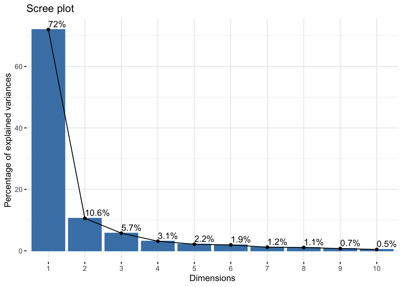

Past versions of summer_winterpca-1.png

Version	Author	Date
d9fb6da	Lily Heald	2025-02-04

fviz_pca_var(reflectancepcaws, col.var = "black")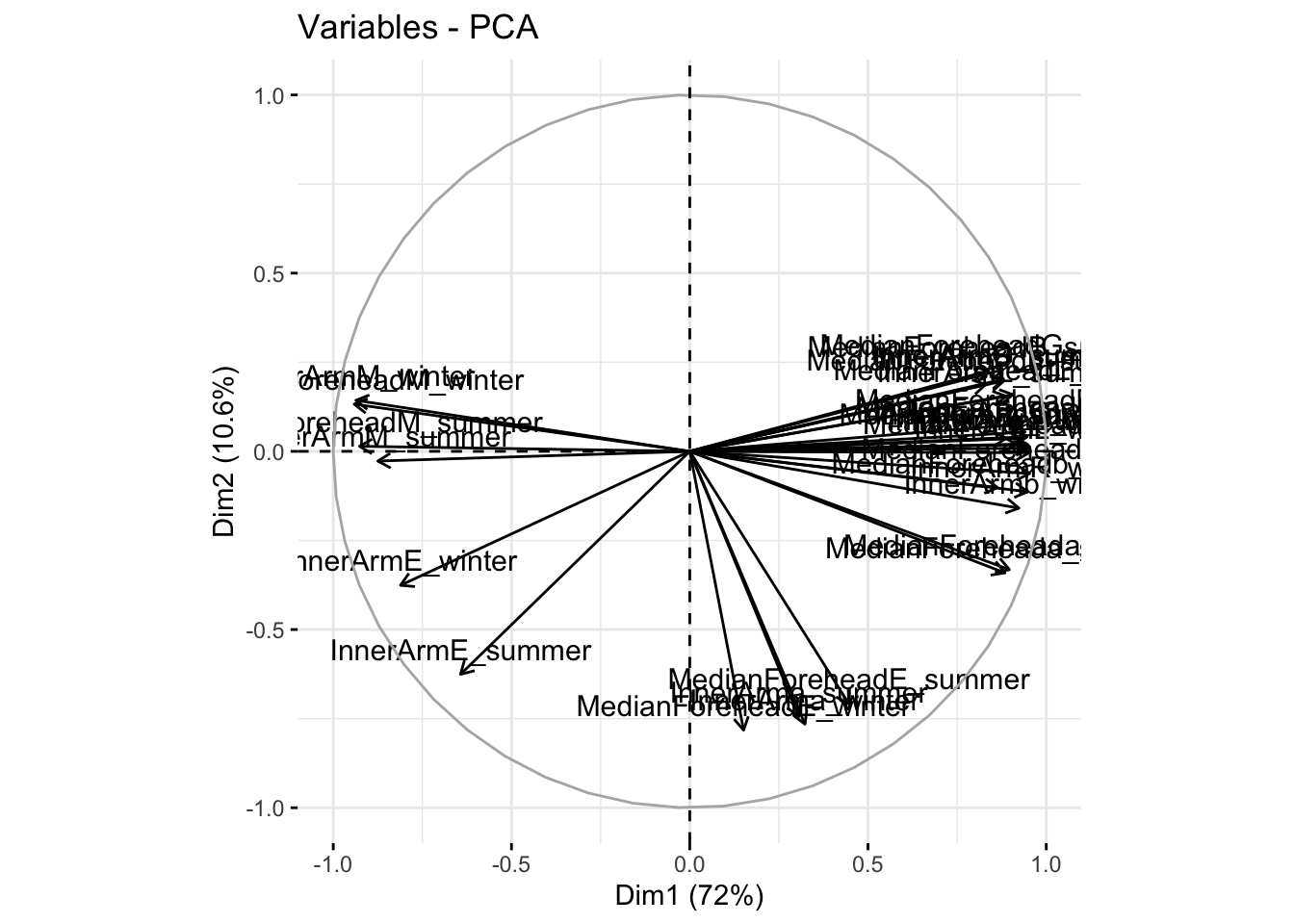

Past versions of summer_winterpca-2.png

Version	Author	Date
d9fb6da	Lily Heald	2025-02-04

fviz_cos2(reflectancepcaws, choice = "var", axes = 1:2)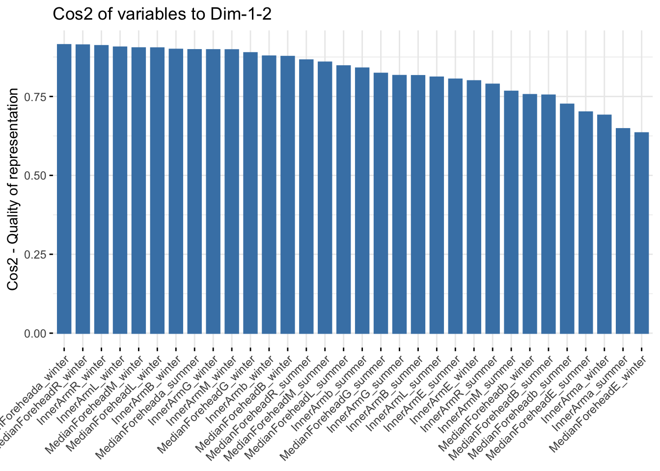

Past versions of summer_winterpca-3.png

Version	Author	Date
d9fb6da	Lily Heald	2025-02-04

wscomps <- as.data.frame(reflectancepcaws$x)
reflectance_ws <- cbind(summer_winter_clean,wscomps[,c(1,2)])
reflectance_ws <- reflectance_ws %>%
  select(-matches("SkinReflectance"))
reflectance_ws <- reflectance_ws %>%
  select(-"Ethnicity_winter")
names(reflectance_ws)[names(reflectance_ws) == 'Ethnicity_summer'] <- 'Ethnicity'



ggplot(reflectance_ws, aes(x=PC1, y=PC2, col = Ethnicity, fill = Ethnicity)) +
  stat_ellipse(geom = "polygon", col= "black", alpha =0.5)+
  geom_point(shape=21, col="black") +
  labs(title = "Wide Pigmentation PCA")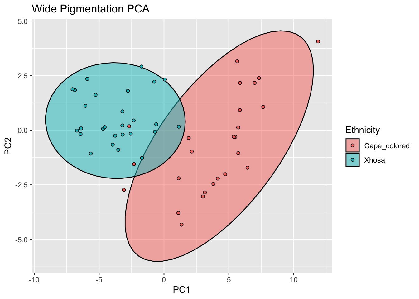

Past versions of wspcavis-1.png

Version	Author	Date
d9fb6da	Lily Heald	2025-02-04

fviz_contrib(reflectancepcaws, choice = "var", axes = 1, top = 20)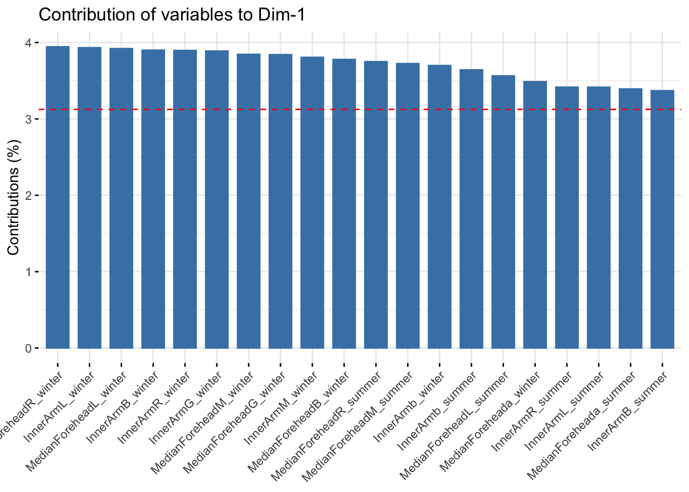

Past versions of wspcavis-2.png

Version	Author	Date
d9fb6da	Lily Heald	2025-02-04

fviz_contrib(reflectancepcaws, choice = "var", axes = 2, top = 20)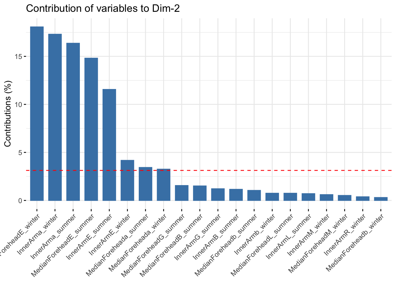

Past versions of wspcavis-3.png

Version	Author	Date
d9fb6da	Lily Heald	2025-02-04

pigmentation subset

summer_refl_metrics <- summer_data %>%
  select(matches("InnerArm|MedianForehead"))
summer_refl_metrics <- na.omit(summer_refl_metrics)

winter_refl_metrics <- winter_data %>%
  select(matches("InnerArm|MedianForehead"))
winter_refl_metrics <- na.omit(winter_refl_metrics)

six_refl_metrics <- six_week_data %>%
  select(matches("InnerArm|MedianForehead"))
six_refl_metrics <- na.omit(six_refl_metrics)

six_refl <- scale(six_refl_metrics)
six_refl_pca <- prcomp(six_refl)
summary(six_refl_pca)

Importance of components:
                         PC1    PC2     PC3     PC4     PC5     PC6     PC7
Standard deviation     3.237 1.6206 1.06822 0.99730 0.54065 0.43093 0.36791
Proportion of Variance 0.655 0.1641 0.07132 0.06216 0.01827 0.01161 0.00846
Cumulative Proportion  0.655 0.8191 0.89045 0.95261 0.97088 0.98248 0.99094
                          PC8     PC9    PC10    PC11    PC12    PC13    PC14
Standard deviation     0.2467 0.19478 0.13699 0.10300 0.08596 0.06440 0.04847
Proportion of Variance 0.0038 0.00237 0.00117 0.00066 0.00046 0.00026 0.00015
Cumulative Proportion  0.9948 0.99712 0.99829 0.99895 0.99942 0.99967 0.99982
                          PC15    PC16
Standard deviation     0.04121 0.03399
Proportion of Variance 0.00011 0.00007
Cumulative Proportion  0.99993 1.00000

six_refl_pca$loadings[, 1:2]

NULL

fviz_eig(six_refl_pca, addlabels = TRUE)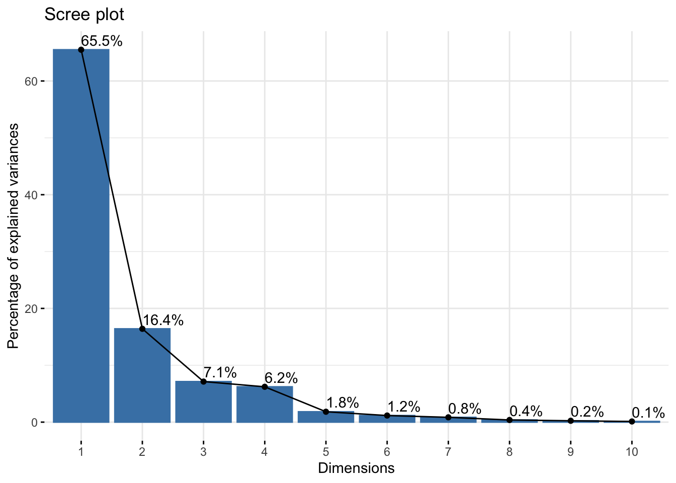

Past versions of sixpigpca-1.png

Version	Author	Date
d9fb6da	Lily Heald	2025-02-04

fviz_pca_var(six_refl_pca, col.var = "black")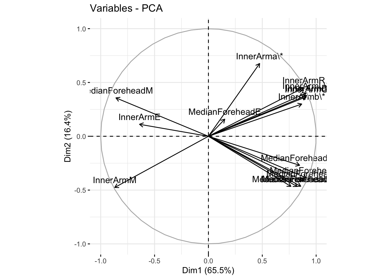

Past versions of sixpigpca-2.png

Version	Author	Date
d9fb6da	Lily Heald	2025-02-04

fviz_cos2(six_refl_pca, choice = "var", axes = 1:2)

Past versions of sixpigpca-3.png

Version	Author	Date
d9fb6da	Lily Heald	2025-02-04

six_pigm_comps <- as.data.frame(six_refl_pca$x)
six_pigment <- cbind(six_week_data,six_pigm_comps[,c(1,2)])

ggplot(six_pigment, aes(x=PC1, y=PC2, col = Ethnicity, fill = Ethnicity)) +
  stat_ellipse(geom = "polygon", col= "black", alpha =0.5)+
  geom_point(shape=21, col="black") +
  labs(title = "Six Week Pigmentation PCA")

Past versions of sixpigcomps-1.png

Version	Author	Date
d9fb6da	Lily Heald	2025-02-04

fviz_contrib(six_refl_pca, choice = "var", axes = 1, top = 10)

Past versions of sixpigcomps-2.png

Version	Author	Date
d9fb6da	Lily Heald	2025-02-04

fviz_contrib(six_refl_pca, choice = "var", axes = 2, top = 10)

Past versions of sixpigcomps-3.png

Version	Author	Date
d9fb6da	Lily Heald	2025-02-04

summer_refl <- scale(summer_refl_metrics)
summer_refl_pca <- prcomp(summer_refl)
summary(summer_refl_pca)

Importance of components:
                          PC1    PC2     PC3     PC4     PC5    PC6     PC7
Standard deviation     3.4053 1.3280 1.23143 0.78241 0.52805 0.3175 0.20528
Proportion of Variance 0.7248 0.1102 0.09478 0.03826 0.01743 0.0063 0.00263
Cumulative Proportion  0.7248 0.8350 0.92975 0.96801 0.98543 0.9917 0.99437
                           PC8     PC9    PC10    PC11    PC12    PC13    PC14
Standard deviation     0.17041 0.15034 0.11867 0.09491 0.08545 0.05918 0.04667
Proportion of Variance 0.00182 0.00141 0.00088 0.00056 0.00046 0.00022 0.00014
Cumulative Proportion  0.99618 0.99760 0.99848 0.99904 0.99949 0.99971 0.99985
                          PC15    PC16
Standard deviation     0.03646 0.03273
Proportion of Variance 0.00008 0.00007
Cumulative Proportion  0.99993 1.00000

summer_refl_pca$loadings[, 1:2]

NULL

fviz_eig(summer_refl_pca, addlabels = TRUE)

Past versions of summerpigpca-1.png

Version	Author	Date
d9fb6da	Lily Heald	2025-02-04

fviz_pca_var(summer_refl_pca, col.var = "black")

Past versions of summerpigpca-2.png

Version	Author	Date
d9fb6da	Lily Heald	2025-02-04

fviz_cos2(summer_refl_pca, choice = "var", axes = 1:2)

Past versions of summerpigpca-3.png

Version	Author	Date
d9fb6da	Lily Heald	2025-02-04

summer_pigm_comps <- as.data.frame(summer_refl_pca$x)
summer_pigment <- cbind(summer_data,summer_pigm_comps[,c(1,2)])

ggplot(summer_pigment, aes(x=PC1, y=PC2, col = Ethnicity, fill = Ethnicity)) +
  stat_ellipse(geom = "polygon", col= "black", alpha =0.5)+
  geom_point(shape=21, col="black") +
  labs(title = "Summer Pigmentation PCA")

Past versions of summerpigcomps-1.png

Version	Author	Date
d9fb6da	Lily Heald	2025-02-04

fviz_contrib(summer_refl_pca, choice = "var", axes = 1, top = 10)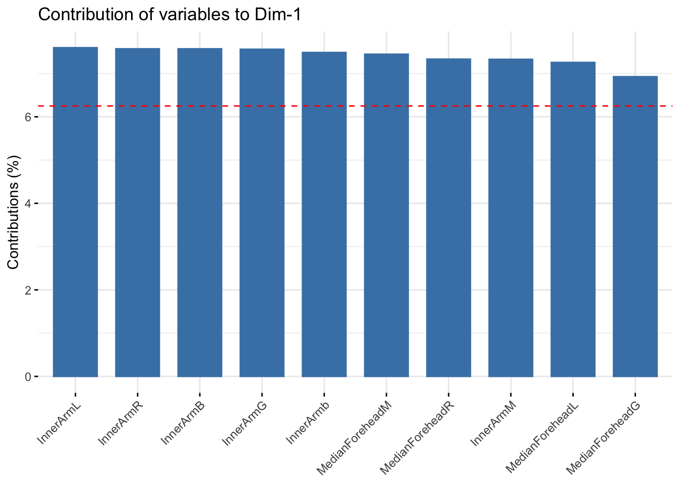

Past versions of summerpigcomps-2.png

Version	Author	Date
d9fb6da	Lily Heald	2025-02-04

fviz_contrib(summer_refl_pca, choice = "var", axes = 2, top = 10)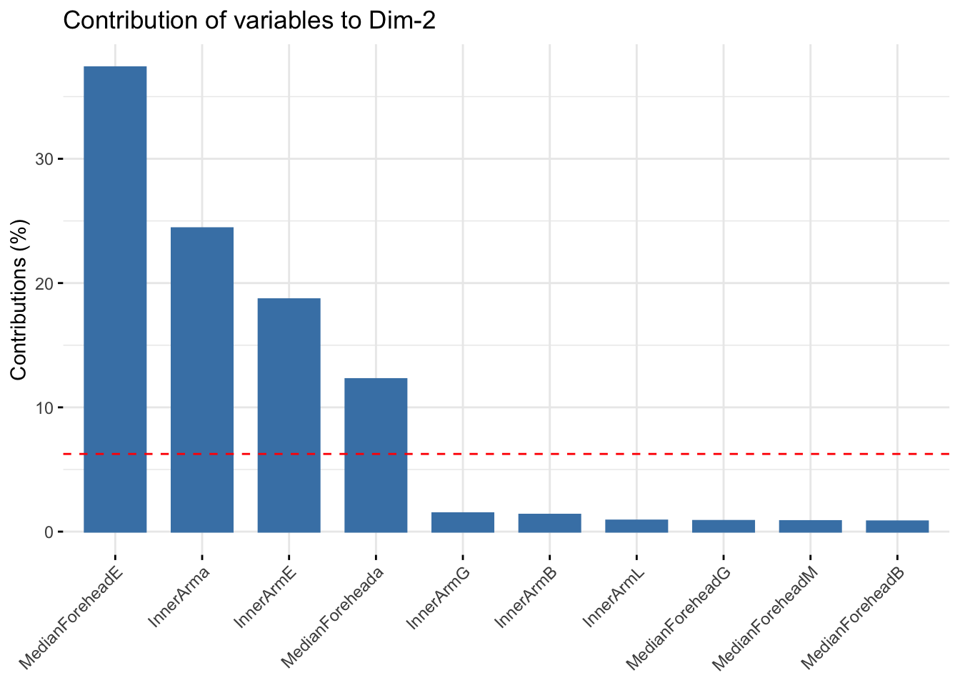

Past versions of summerpigcomps-3.png

Version	Author	Date
d9fb6da	Lily Heald	2025-02-04

winter_refl <- scale(winter_refl_metrics)
winter_refl_pca <- prcomp(winter_refl)
summary(winter_refl_pca)

Importance of components:
                          PC1    PC2     PC3     PC4     PC5     PC6     PC7
Standard deviation     3.5551 1.3839 0.80737 0.64068 0.48775 0.26632 0.15397
Proportion of Variance 0.7899 0.1197 0.04074 0.02565 0.01487 0.00443 0.00148
Cumulative Proportion  0.7899 0.9096 0.95038 0.97603 0.99090 0.99534 0.99682
                           PC8     PC9    PC10    PC11    PC12    PC13    PC14
Standard deviation     0.14316 0.12764 0.07986 0.06160 0.03646 0.03546 0.02830
Proportion of Variance 0.00128 0.00102 0.00040 0.00024 0.00008 0.00008 0.00005
Cumulative Proportion  0.99810 0.99912 0.99952 0.99975 0.99984 0.99991 0.99996
                          PC15    PC16
Standard deviation     0.01758 0.01615
Proportion of Variance 0.00002 0.00002
Cumulative Proportion  0.99998 1.00000

winter_refl_pca$loadings[, 1:2]

NULL

fviz_eig(winter_refl_pca, addlabels = TRUE)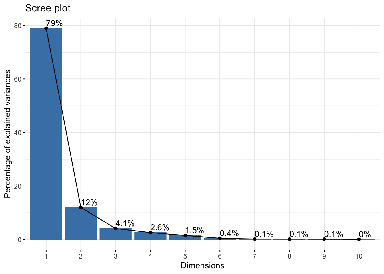

Past versions of winterpigpca-1.png

Version	Author	Date
d9fb6da	Lily Heald	2025-02-04

fviz_pca_var(winter_refl_pca, col.var = "black")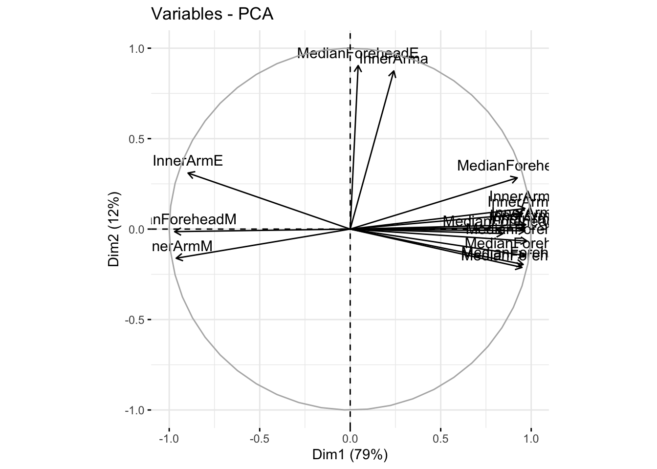

Past versions of winterpigpca-2.png

Version	Author	Date
d9fb6da	Lily Heald	2025-02-04

fviz_cos2(winter_refl_pca, choice = "var", axes = 1:2)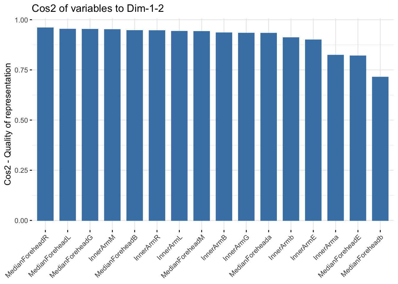

Past versions of winterpigpca-3.png

Version	Author	Date
d9fb6da	Lily Heald	2025-02-04

winter_pigm_comps <- as.data.frame(winter_refl_pca$x)
winter_pigment <- cbind(winter_data,winter_pigm_comps[,c(1,2)])

ggplot(winter_pigment, aes(x=PC1, y=PC2, col = Ethnicity, fill = Ethnicity)) +
  stat_ellipse(geom = "polygon", col= "black", alpha =0.5)+
  geom_point(shape=21, col="black") +
  labs(title = "Winter Pigmentation PCA")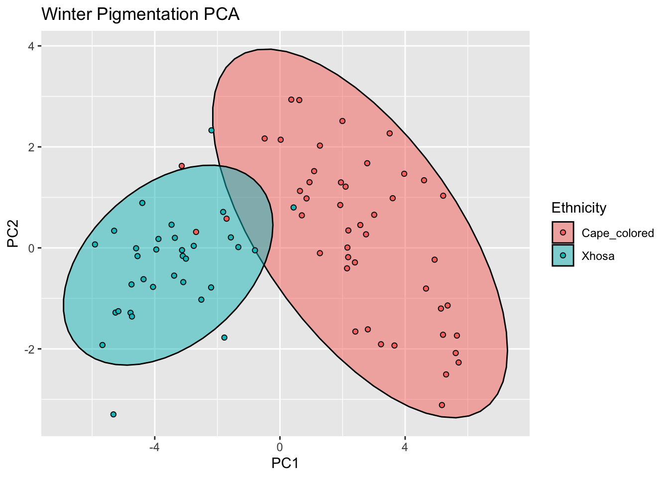

Past versions of winterpigcomps-1.png

Version	Author	Date
d9fb6da	Lily Heald	2025-02-04

fviz_contrib(winter_refl_pca, choice = "var", axes = 1, top = 10)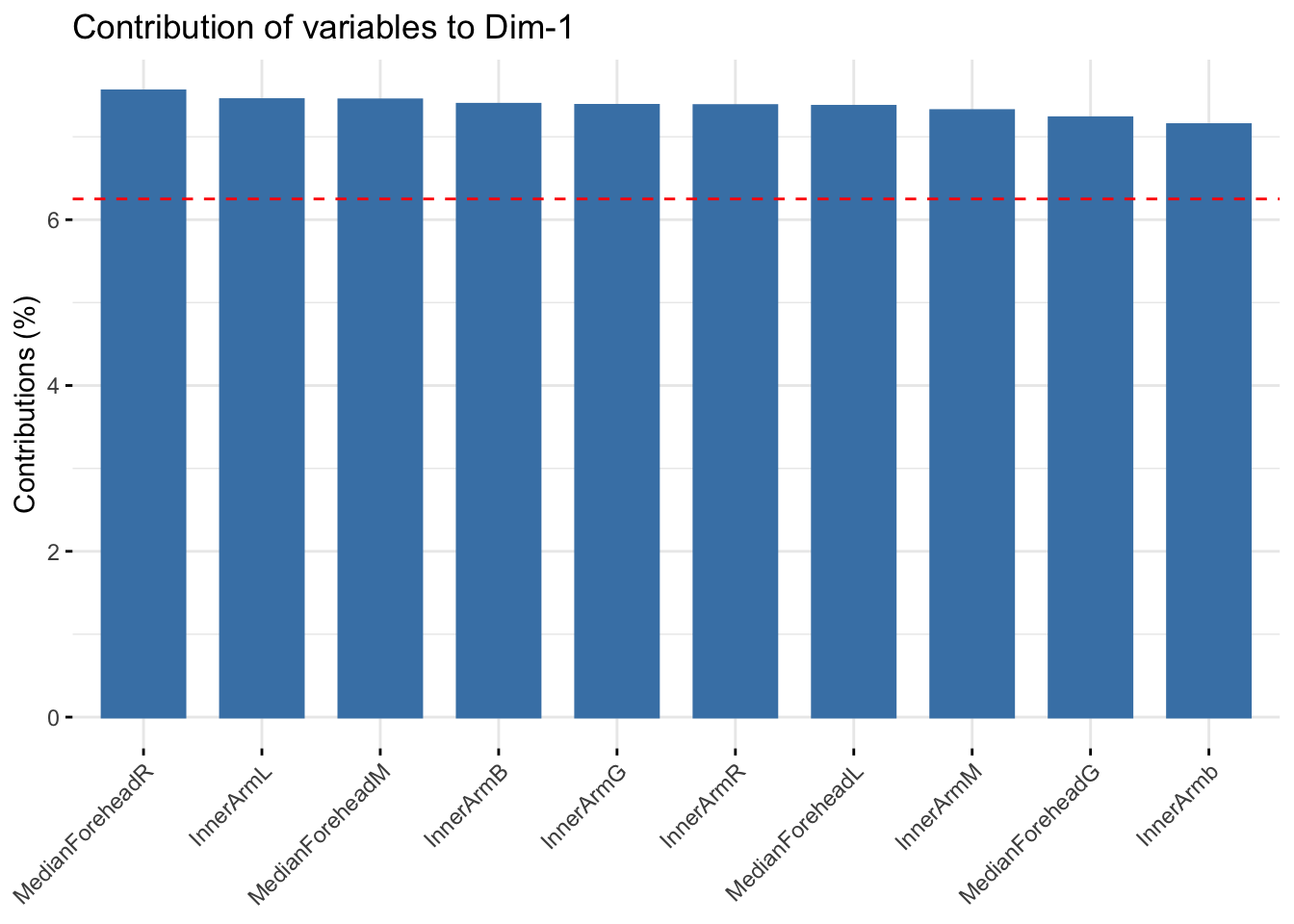

Past versions of winterpigcomps-2.png

Version	Author	Date
d9fb6da	Lily Heald	2025-02-04

fviz_contrib(winter_refl_pca, choice = "var", axes = 2, top = 10)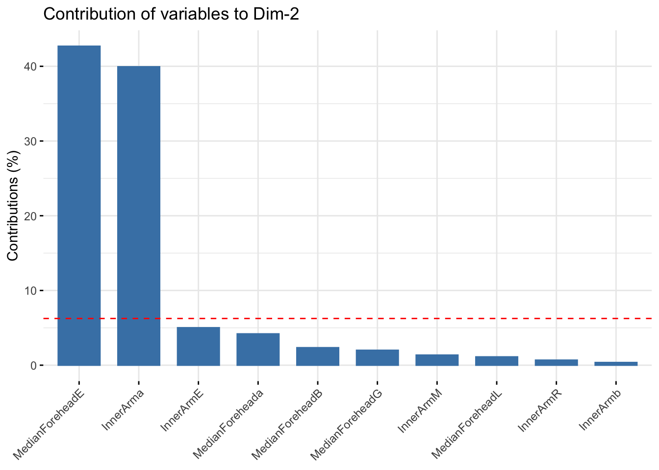

Past versions of winterpigcomps-3.png

Version	Author	Date
d9fb6da	Lily Heald	2025-02-04

RGB subset

summer_winter_clean <- na.omit(summer_winter)
reflectance_rgb_ws <- summer_winter_clean %>%
  select(matches("MedianForeheadR|MedianForeheadG|MedianForeheadB|InnerArmR|InnerArmG|InnerArmB", ignore.case = FALSE))

reflectance4 <- scale(reflectance_rgb_ws)
reflectancergbws <- prcomp(reflectance4)
summary(reflectancergbws)

Importance of components:
                          PC1     PC2     PC3     PC4    PC5     PC6     PC7
Standard deviation     3.1878 0.94496 0.72698 0.51980 0.2593 0.19373 0.12847
Proportion of Variance 0.8468 0.07441 0.04404 0.02252 0.0056 0.00313 0.00138
Cumulative Proportion  0.8468 0.92126 0.96530 0.98782 0.9934 0.99655 0.99792
                           PC8     PC9    PC10    PC11    PC12
Standard deviation     0.10024 0.08260 0.07502 0.04244 0.02558
Proportion of Variance 0.00084 0.00057 0.00047 0.00015 0.00005
Cumulative Proportion  0.99876 0.99933 0.99980 0.99995 1.00000

reflectancergbws$loadings[, 1:2]

NULL

fviz_eig(reflectancergbws, addlabels = TRUE)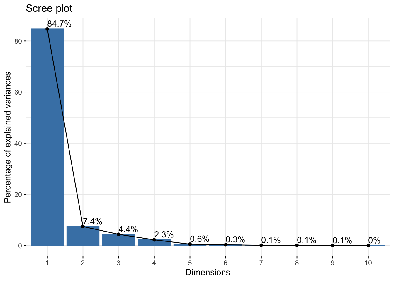

Past versions of seasonalrgb-1.png

Version	Author	Date
d9fb6da	Lily Heald	2025-02-04

fviz_pca_var(reflectancergbws, col.var = "black")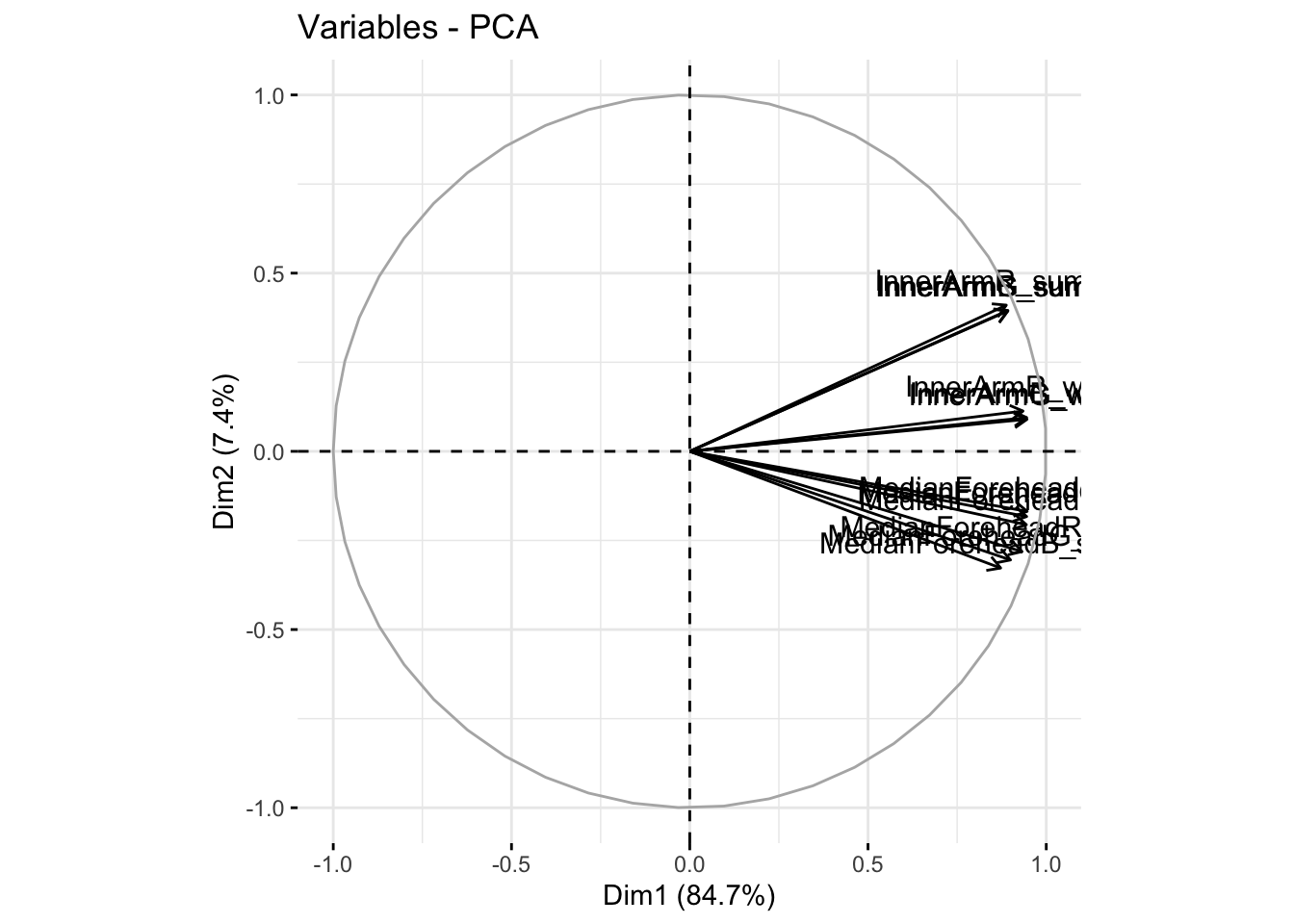

Past versions of seasonalrgb-2.png

Version	Author	Date
d9fb6da	Lily Heald	2025-02-04

fviz_cos2(reflectancergbws, choice = "var", axes = 1:2)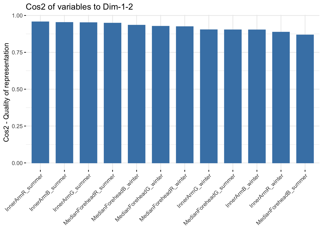

Past versions of seasonalrgb-3.png

Version	Author	Date
d9fb6da	Lily Heald	2025-02-04

wsrgbcomps <- as.data.frame(reflectancergbws$x)
rgb_ws_bind <- cbind(summer_winter_clean,wsrgbcomps[,c(1,2)])
rgb_ws_bind <- rgb_ws_bind %>%
  select(-matches("SkinReflectance"))
rgb_ws_bind <- rgb_ws_bind %>%
  select(-"Ethnicity_winter")
names(rgb_ws_bind)[names(rgb_ws_bind) == 'Ethnicity_summer'] <- 'Ethnicity'


ggplot(rgb_ws_bind, aes(x=PC1, y=PC2, col = Ethnicity, fill = Ethnicity)) +
  stat_ellipse(geom = "polygon", col= "black", alpha =0.5)+
  geom_point(shape=21, col="black") +
  labs(title = "Wide Pigmentation PCA")

Past versions of wsrgbvis-1.png

Version	Author	Date
d9fb6da	Lily Heald	2025-02-04

fviz_contrib(reflectancergbws, choice = "var", axes = 1, top = 20)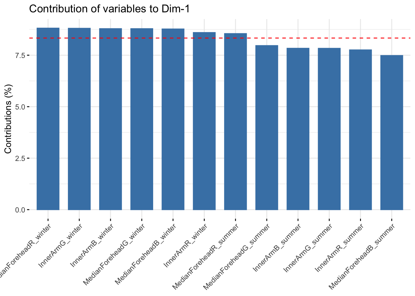

Past versions of wsrgbvis-2.png

Version	Author	Date
d9fb6da	Lily Heald	2025-02-04

fviz_contrib(reflectancergbws, choice = "var", axes = 2, top = 20)

Past versions of wsrgbvis-3.png

Version	Author	Date
d9fb6da	Lily Heald	2025-02-04

summer_rgb <- summer_data %>%
  select(matches("ForeheadR|ForeheadG|ForeheadB|InnerArmR|InnerArmG|InnerArmB", ignore.case = FALSE))
summer_rgb <- na.omit(summer_rgb)

winter_rgb <- winter_data %>%
  select(matches("ForeheadR|ForeheadG|ForeheadB|InnerArmR|InnerArmG|InnerArmB", ignore.case = FALSE))
winter_rgb <- na.omit(winter_rgb)

six_rgb <- six_week_data %>%
  select(matches("ForeheadR|ForeheadG|ForeheadB|InnerArmR|InnerArmG|InnerArmB", ignore.case = FALSE))
six_rgb <- na.omit(six_rgb)

winter_rgb_scale <- scale(winter_rgb)
winter_rgb_pca <- prcomp(winter_rgb_scale)
summary(winter_rgb_pca)

Importance of components:
                          PC1     PC2     PC3     PC4     PC5     PC6
Standard deviation     2.3720 0.58112 0.15130 0.08075 0.07684 0.01941
Proportion of Variance 0.9378 0.05628 0.00382 0.00109 0.00098 0.00006
Cumulative Proportion  0.9378 0.99405 0.99787 0.99895 0.99994 1.00000

winter_rgb_pca$loadings[, 1:2]

NULL

fviz_eig(winter_rgb_pca, addlabels = TRUE)

Past versions of winterrgbpca-1.png

Version	Author	Date
d9fb6da	Lily Heald	2025-02-04

fviz_pca_var(winter_rgb_pca, col.var = "black")

Past versions of winterrgbpca-2.png

Version	Author	Date
d9fb6da	Lily Heald	2025-02-04

fviz_cos2(winter_rgb_pca, choice = "var", axes = 1:2)

Past versions of winterrgbpca-3.png

Version	Author	Date
d9fb6da	Lily Heald	2025-02-04

winter_rgb_comps <- as.data.frame(winter_rgb_pca$x)
winter_rgb_new <- cbind(winter_data,winter_rgb_comps[,c(1,2)])

ggplot(winter_rgb_new, aes(x=PC1, y=PC2, col = Ethnicity, fill = Ethnicity)) +
  stat_ellipse(geom = "polygon", col= "black", alpha =0.5)+
  geom_point(shape=21, col="black") +
  labs(title = "Winter RGB PCA")

Past versions of winterrgbcomps-1.png

Version	Author	Date
d9fb6da	Lily Heald	2025-02-04

fviz_contrib(winter_rgb_pca, choice = "var", axes = 1, top = 10)

Past versions of winterrgbcomps-2.png

Version	Author	Date
d9fb6da	Lily Heald	2025-02-04

fviz_contrib(winter_rgb_pca, choice = "var", axes = 2, top = 10)

Past versions of winterrgbcomps-3.png

Version	Author	Date
d9fb6da	Lily Heald	2025-02-04

summer_rgb_scale <- scale(summer_rgb)
summer_rgb_pca <- prcomp(summer_rgb_scale)
summary(summer_rgb_pca)

Importance of components:
                          PC1    PC2     PC3     PC4     PC5     PC6
Standard deviation     2.2617 0.8751 0.26995 0.17017 0.11981 0.05129
Proportion of Variance 0.8526 0.1277 0.01215 0.00483 0.00239 0.00044
Cumulative Proportion  0.8526 0.9802 0.99234 0.99717 0.99956 1.00000

summer_rgb_pca$loadings[, 1:2]

NULL

fviz_eig(summer_rgb_pca, addlabels = TRUE)

Past versions of summergbpca-1.png

Version	Author	Date
d9fb6da	Lily Heald	2025-02-04

fviz_pca_var(summer_rgb_pca, col.var = "black")

Past versions of summergbpca-2.png

Version	Author	Date
d9fb6da	Lily Heald	2025-02-04

fviz_cos2(summer_rgb_pca, choice = "var", axes = 1:2)

Past versions of summergbpca-3.png

Version	Author	Date
d9fb6da	Lily Heald	2025-02-04

summer_rgb_comps <- as.data.frame(summer_rgb_pca$x)
summer_rgb_new <- cbind(summer_data,summer_rgb_comps[,c(1,2)])

ggplot(summer_rgb_new, aes(x=PC1, y=PC2, col = Ethnicity, fill = Ethnicity)) +
  stat_ellipse(geom = "polygon", col= "black", alpha =0.5)+
  geom_point(shape=21, col="black") +
  labs(title = "Summer RGB PCA")

Past versions of summerrgbcomps-1.png

Version	Author	Date
d9fb6da	Lily Heald	2025-02-04

fviz_contrib(summer_rgb_pca, choice = "var", axes = 1, top = 10)

Past versions of summerrgbcomps-2.png

Version	Author	Date
d9fb6da	Lily Heald	2025-02-04

fviz_contrib(summer_rgb_pca, choice = "var", axes = 2, top = 10)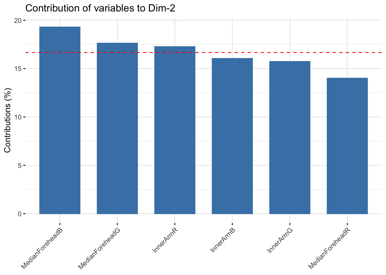

Past versions of summerrgbcomps-3.png

Version	Author	Date
d9fb6da	Lily Heald	2025-02-04

six_rgb_scale <- scale(six_rgb)
six_rgb_pca <- prcomp(six_rgb_scale)
summary(six_rgb_pca)

Importance of components:
                          PC1    PC2     PC3     PC4     PC5     PC6
Standard deviation     2.1876 1.0663 0.18148 0.14888 0.13270 0.06947
Proportion of Variance 0.7976 0.1895 0.00549 0.00369 0.00293 0.00080
Cumulative Proportion  0.7976 0.9871 0.99257 0.99626 0.99920 1.00000

six_rgb_pca$loadings[, 1:2]

NULL

fviz_eig(six_rgb_pca, addlabels = TRUE)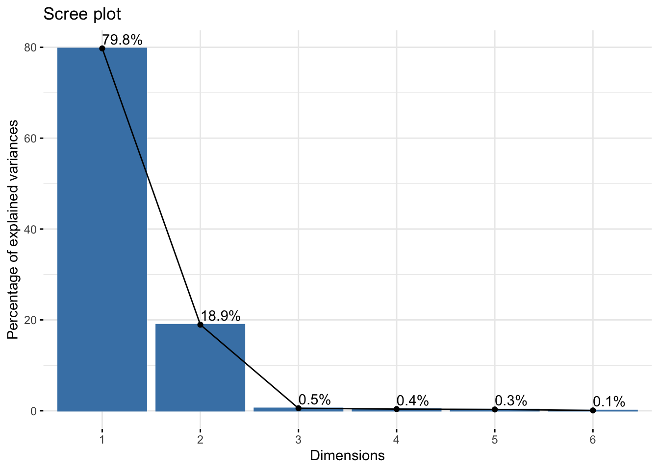

Past versions of sixrgbpca-1.png

Version	Author	Date
d9fb6da	Lily Heald	2025-02-04

fviz_pca_var(six_rgb_pca, col.var = "black")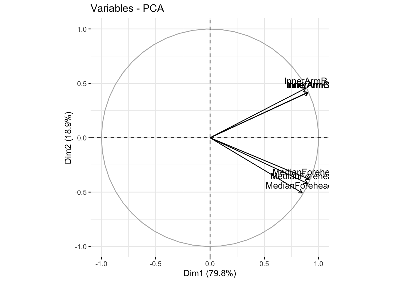

Past versions of sixrgbpca-2.png

Version	Author	Date
d9fb6da	Lily Heald	2025-02-04

fviz_cos2(six_rgb_pca, choice = "var", axes = 1:2)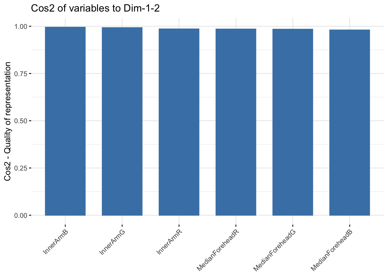

Past versions of sixrgbpca-3.png

Version	Author	Date
d9fb6da	Lily Heald	2025-02-04

six_rgb_comps <- as.data.frame(six_rgb_pca$x)
six_rgb_new <- cbind(six_week_data,six_rgb_comps[,c(1,2)])

ggplot(six_rgb_new, aes(x=PC1, y=PC2, col = Ethnicity, fill = Ethnicity)) +
  stat_ellipse(geom = "polygon", col= "black", alpha =0.5)+
  geom_point(shape=21, col="black") +
  labs(title = "Six Week RGB PCA")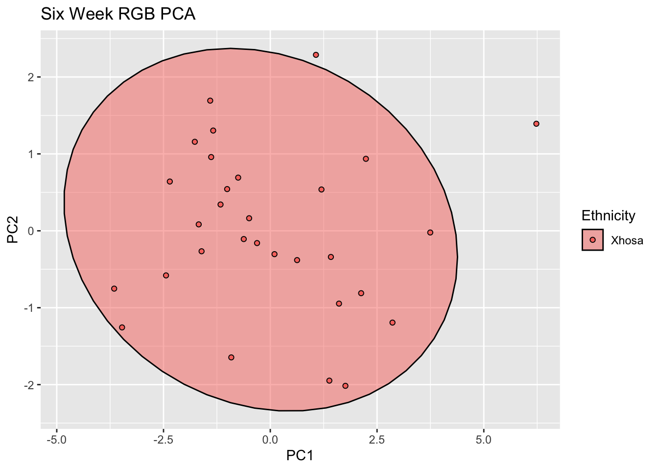

Past versions of sixgbcomps-1.png

Version	Author	Date
d9fb6da	Lily Heald	2025-02-04

fviz_contrib(six_rgb_pca, choice = "var", axes = 1, top = 10)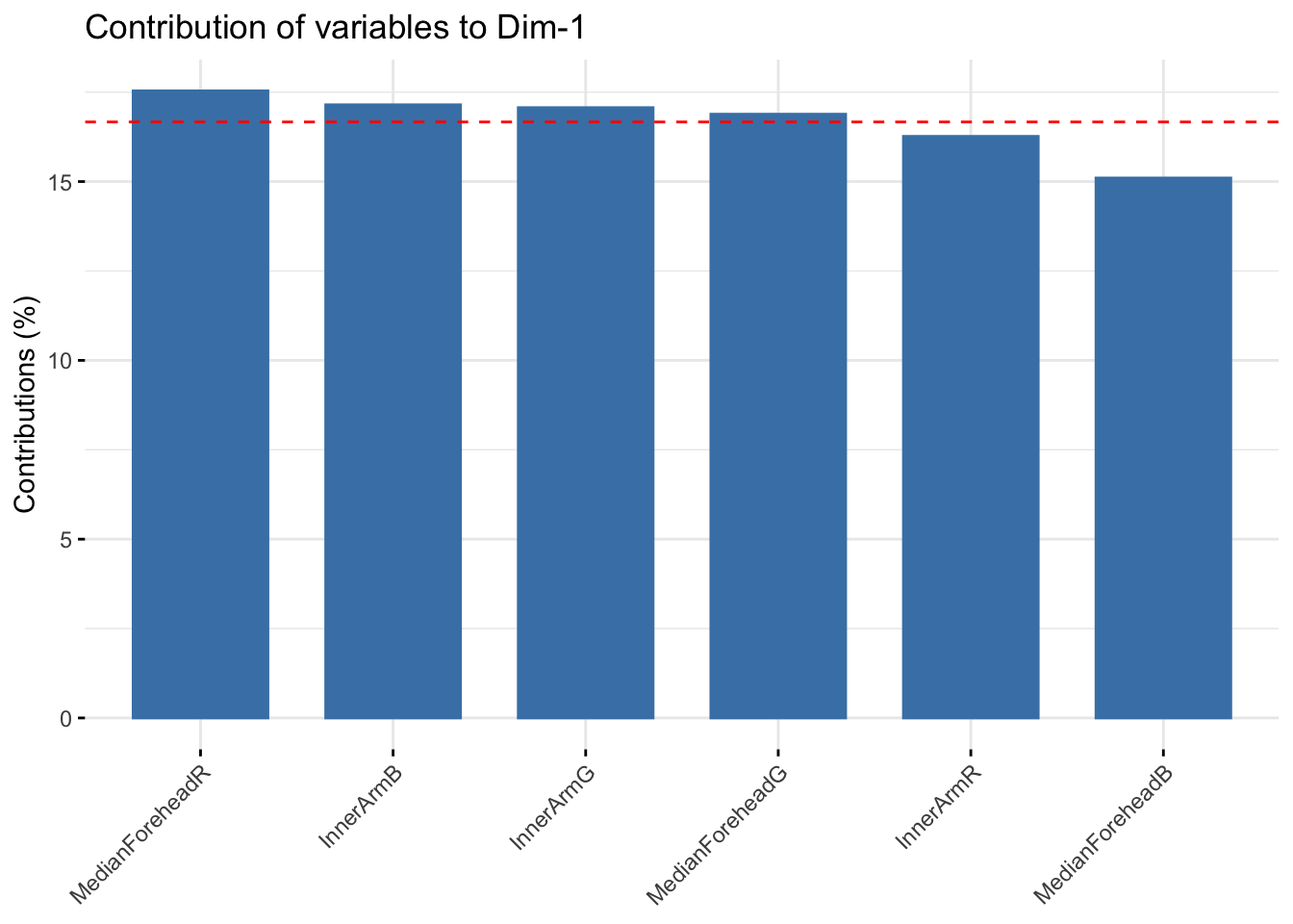

Past versions of sixgbcomps-2.png

Version	Author	Date
d9fb6da	Lily Heald	2025-02-04

fviz_contrib(six_rgb_pca, choice = "var", axes = 2, top = 10)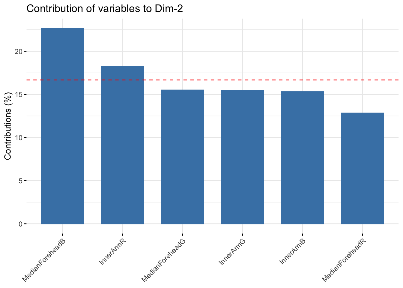

Past versions of sixgbcomps-3.png

Version	Author	Date
d9fb6da	Lily Heald	2025-02-04

CIElab subset

summer_winter_clean <- na.omit(summer_winter)
reflectance_cie_ws <- summer_winter_clean %>%
  select(matches("ForeheadL|Foreheada|Foreheadb|InnerArmL|InnerArma|InnerArmb", ignore.case = FALSE))

reflectance5 <- scale(reflectance_cie_ws)
reflectanceciews <- prcomp(reflectance5)
summary(reflectanceciews)

Importance of components:
                          PC1    PC2     PC3     PC4     PC5     PC6     PC7
Standard deviation     2.9138 1.2773 0.72925 0.60171 0.55023 0.46879 0.42674
Proportion of Variance 0.7075 0.1360 0.04432 0.03017 0.02523 0.01831 0.01518
Cumulative Proportion  0.7075 0.8435 0.88778 0.91795 0.94318 0.96149 0.97667
                           PC8     PC9    PC10    PC11    PC12
Standard deviation     0.31641 0.26634 0.23849 0.16406 0.15854
Proportion of Variance 0.00834 0.00591 0.00474 0.00224 0.00209
Cumulative Proportion  0.98501 0.99092 0.99566 0.99791 1.00000

reflectanceciews$loadings[, 1:2]

NULL

fviz_eig(reflectanceciews, addlabels = TRUE)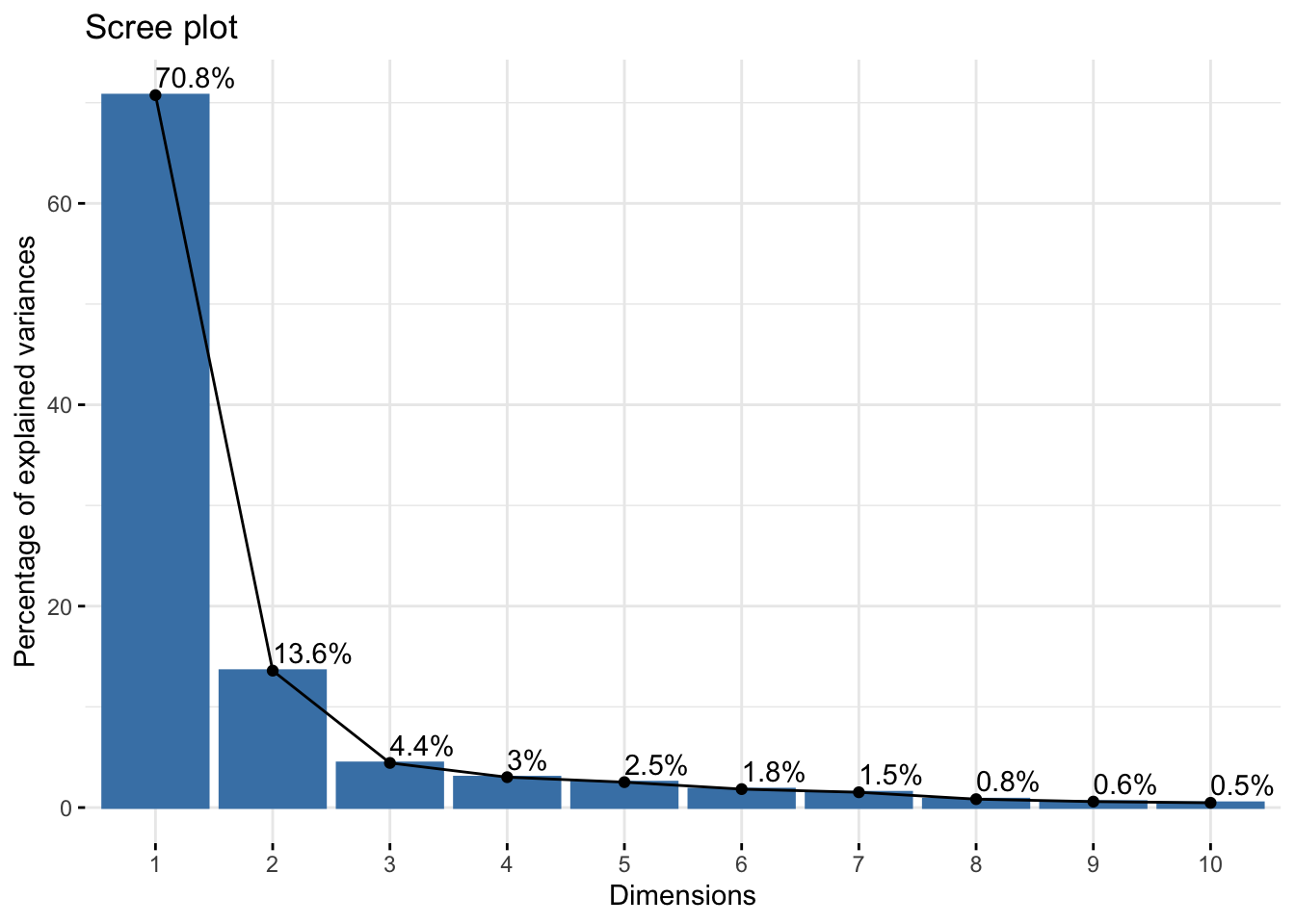

Past versions of seasonalcie-1.png

Version	Author	Date
d9fb6da	Lily Heald	2025-02-04

fviz_pca_var(reflectanceciews, col.var = "black")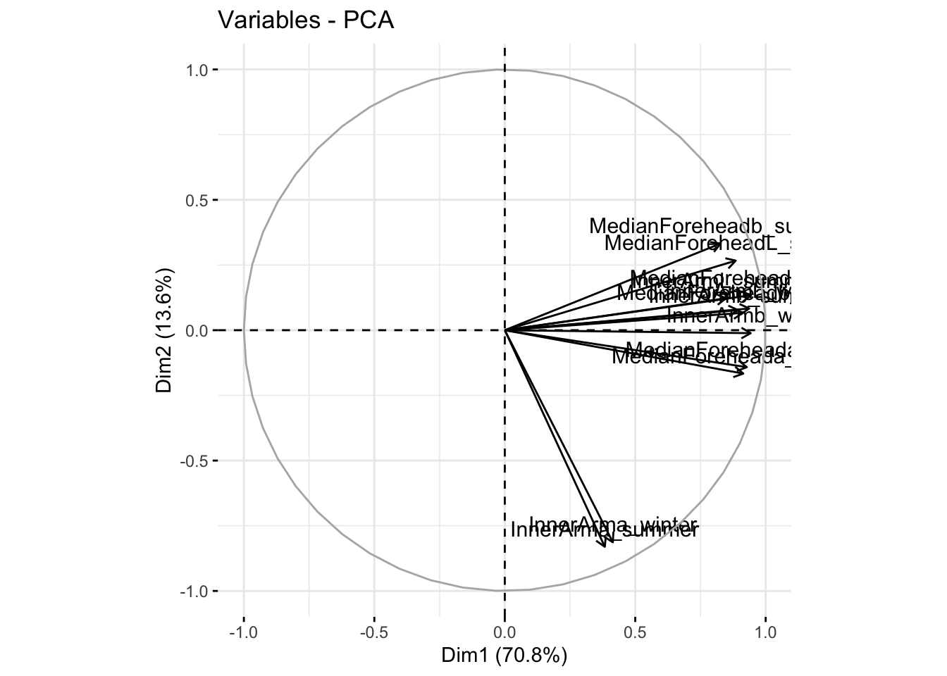

Past versions of seasonalcie-2.png

Version	Author	Date
d9fb6da	Lily Heald	2025-02-04

fviz_cos2(reflectanceciews, choice = "var", axes = 1:2)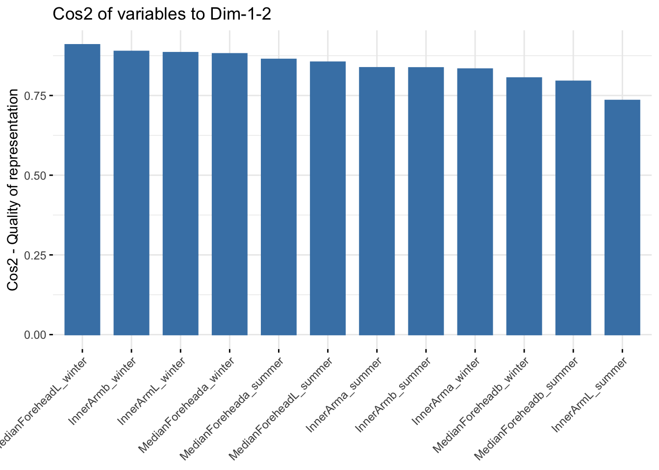

Past versions of seasonalcie-3.png

Version	Author	Date
d9fb6da	Lily Heald	2025-02-04

wsciecomps <- as.data.frame(reflectanceciews$x)
cie_ws_bind <- cbind(summer_winter_clean,wsciecomps[,c(1,2)])
cie_ws_bind <- rgb_ws_bind %>%
  select(-matches("SkinReflectance"))

ggplot(cie_ws_bind, aes(x=PC1, y=PC2, col = Ethnicity, fill = Ethnicity)) +
  stat_ellipse(geom = "polygon", col= "black", alpha =0.5)+
  geom_point(shape=21, col="black") +
  labs(title = "Wide Pigmentation PCA")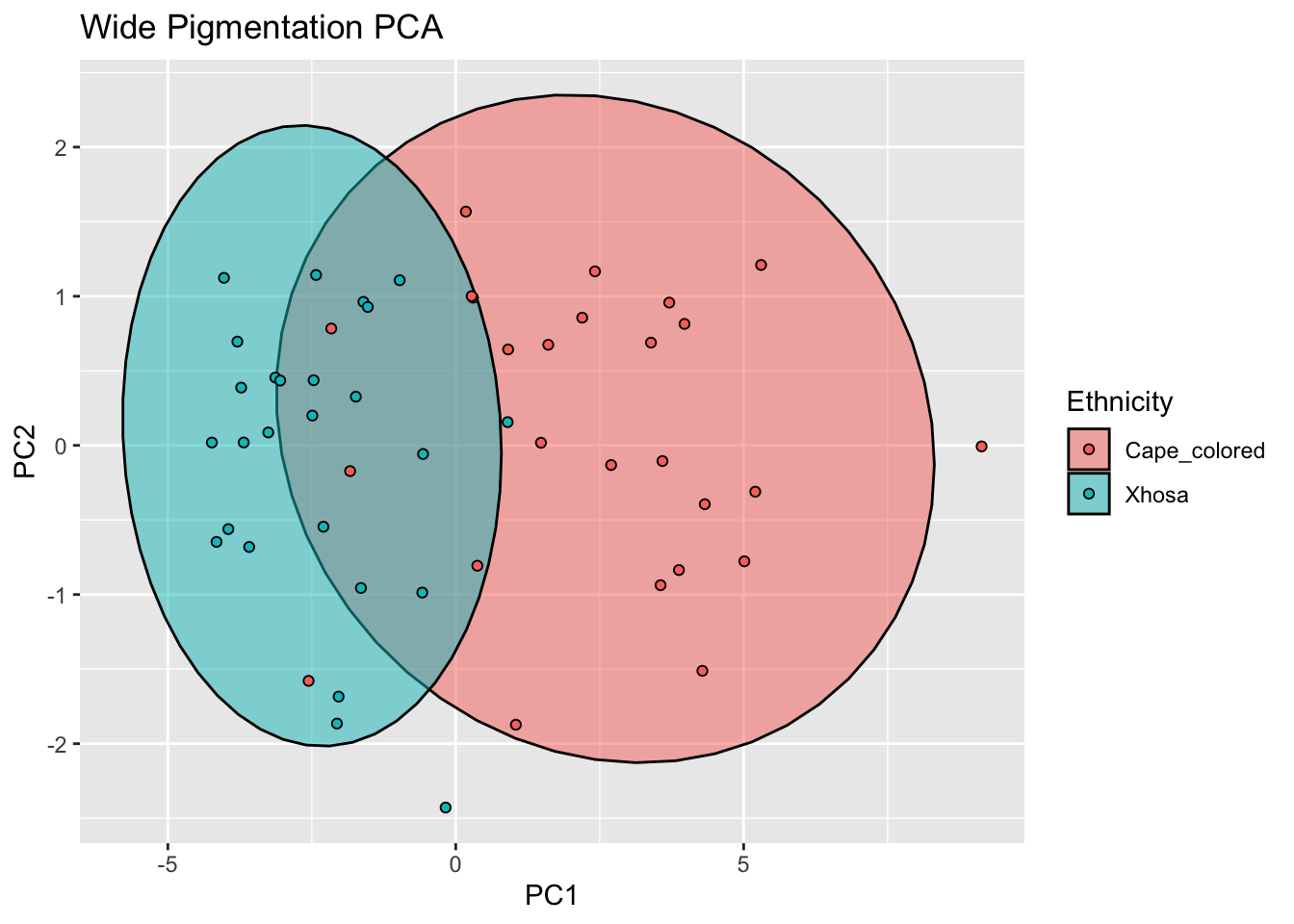

Past versions of wscievis-1.png

Version	Author	Date
d9fb6da	Lily Heald	2025-02-04

fviz_contrib(reflectanceciews, choice = "var", axes = 1, top = 20)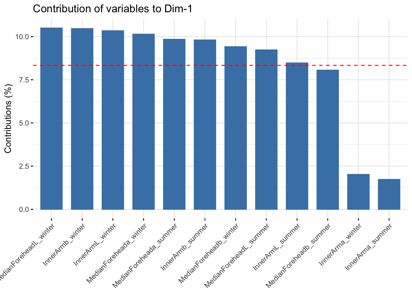

Past versions of wscievis-2.png

Version	Author	Date
d9fb6da	Lily Heald	2025-02-04

fviz_contrib(reflectanceciews, choice = "var", axes = 2, top = 20)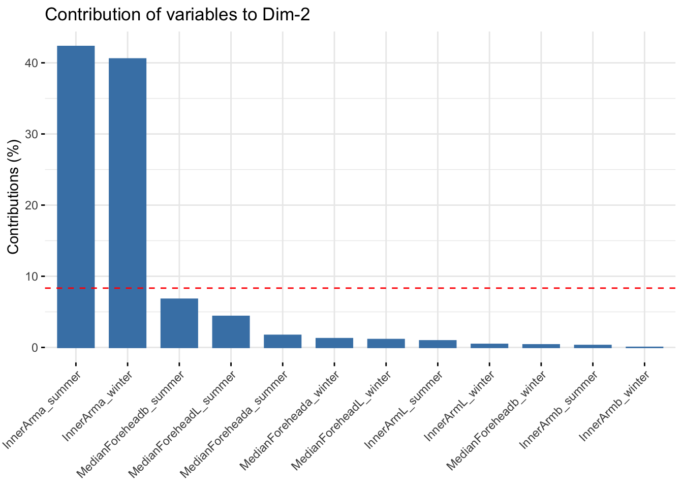

Past versions of wscievis-3.png

Version	Author	Date
d9fb6da	Lily Heald	2025-02-04

summer_cie <- summer_data %>%
  select(matches("ForeheadL|Foreheada|Foreheadb|InnerArmL|InnerArma|InnerArmb", ignore.case = FALSE))
summer_cie <- na.omit(summer_cie)

winter_cie <- winter_data %>%
  select(matches("ForeheadL|Foreheada|Foreheadb|InnerArmL|InnerArma|InnerArmb", ignore.case = FALSE))
winter_cie <- na.omit(winter_cie)

six_cie <- six_week_data %>%
  select(matches("ForeheadL|Foreheada|Foreheadb|InnerArmL|InnerArma|InnerArmb", ignore.case = FALSE))
six_cie <- na.omit(six_cie)

winter_cie_scale <- scale(winter_cie)
winter_cie_pca <- prcomp(winter_cie_scale)
summary(winter_cie_pca)

Importance of components:
                          PC1    PC2    PC3     PC4    PC5     PC6
Standard deviation     2.1257 0.9808 0.5304 0.36540 0.2486 0.20736
Proportion of Variance 0.7531 0.1603 0.0469 0.02225 0.0103 0.00717
Cumulative Proportion  0.7531 0.9134 0.9603 0.98253 0.9928 1.00000

winter_cie_pca$loadings[, 1:2]

NULL

fviz_eig(winter_cie_pca, addlabels = TRUE)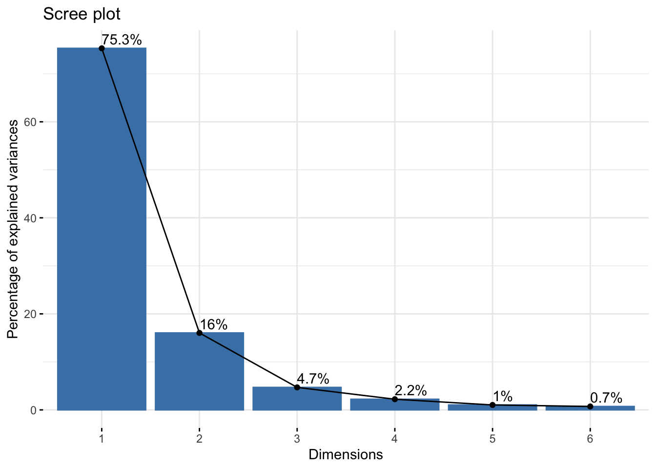

Past versions of winterciepca-1.png

Version	Author	Date
d9fb6da	Lily Heald	2025-02-04

fviz_pca_var(winter_cie_pca, col.var = "black")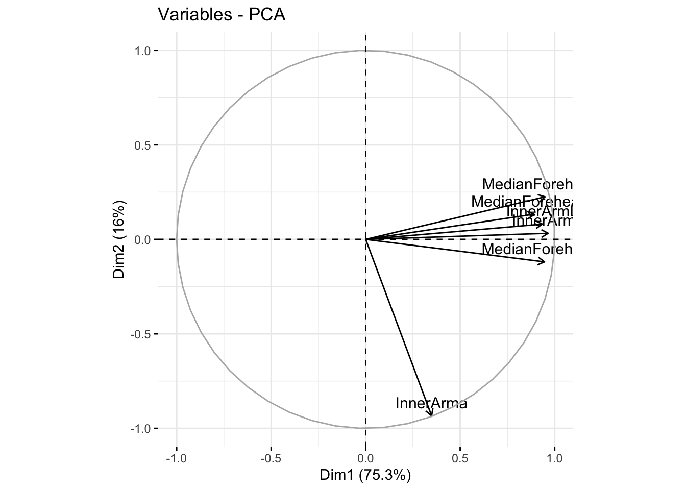

Past versions of winterciepca-2.png

Version	Author	Date
d9fb6da	Lily Heald	2025-02-04

fviz_cos2(winter_cie_pca, choice = "var", axes = 1:2)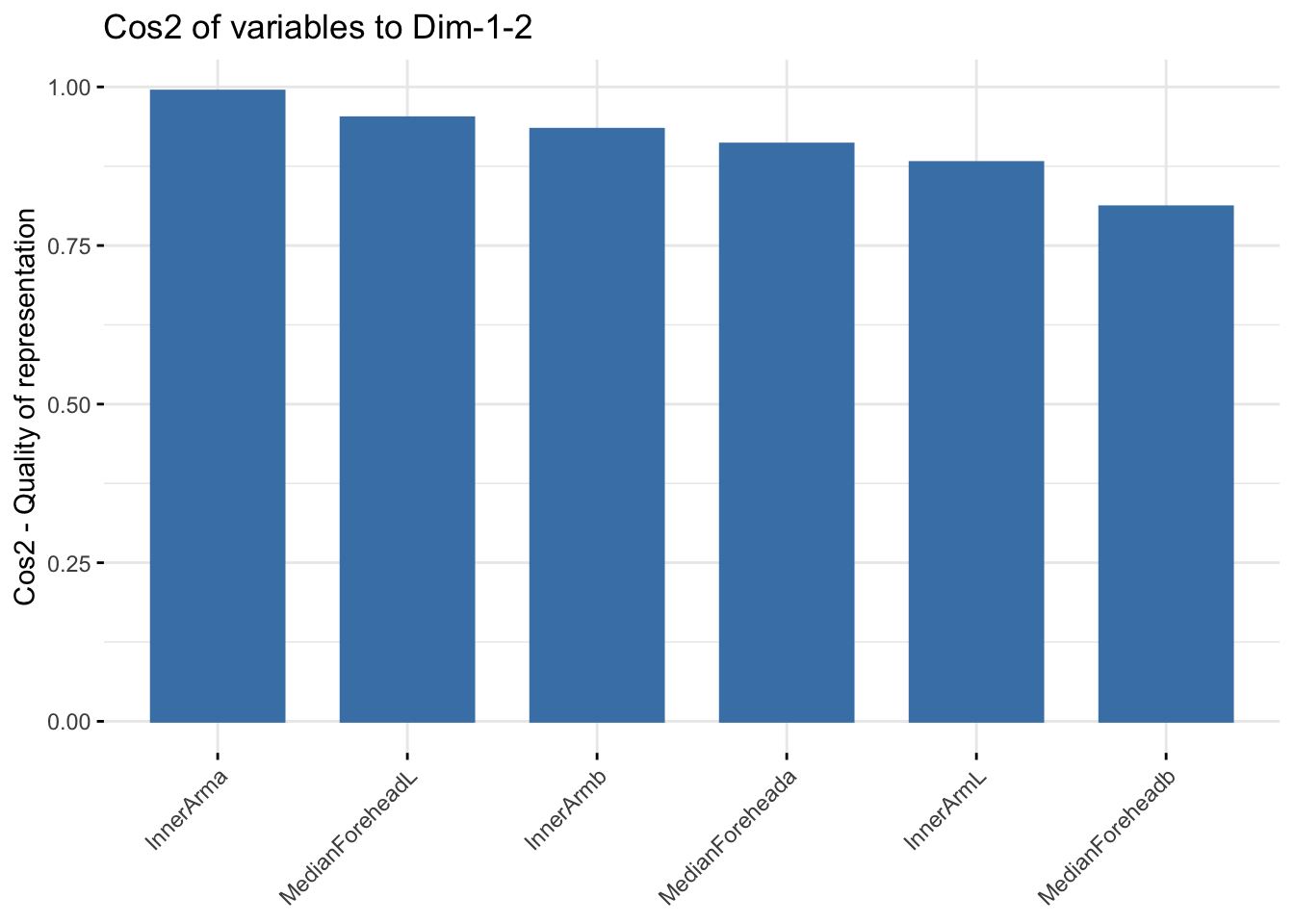

Past versions of winterciepca-3.png

Version	Author	Date
d9fb6da	Lily Heald	2025-02-04

winter_cie_comps <- as.data.frame(winter_cie_pca$x)
winter_cie_new <- cbind(winter_data,winter_cie_comps[,c(1,2)])

ggplot(winter_cie_new, aes(x=PC1, y=PC2, col = Ethnicity, fill = Ethnicity)) +
  stat_ellipse(geom = "polygon", col= "black", alpha =0.5)+
  geom_point(shape=21, col="black") +
  labs(title = "Winter CIELAB PCA")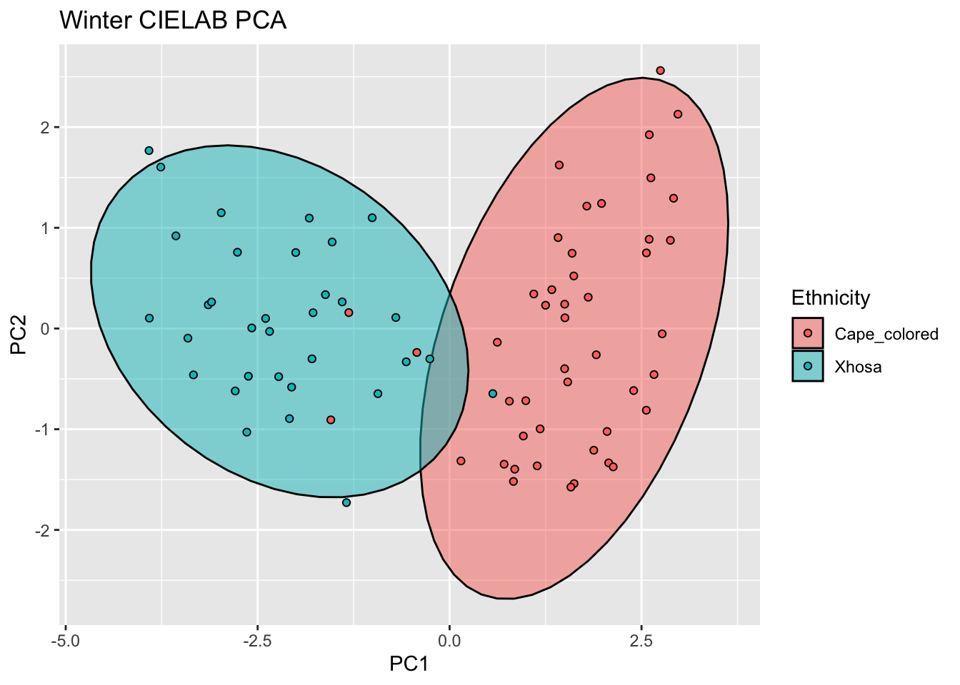

Past versions of winterciecomps-1.png

Version	Author	Date
d9fb6da	Lily Heald	2025-02-04

fviz_contrib(winter_cie_pca, choice = "var", axes = 1, top = 10)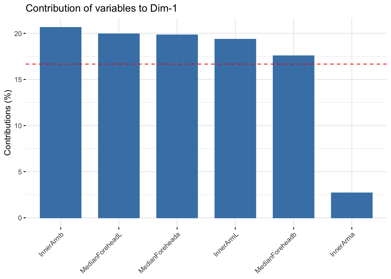

Past versions of winterciecomps-2.png

Version	Author	Date
d9fb6da	Lily Heald	2025-02-04

fviz_contrib(winter_cie_pca, choice = "var", axes = 2, top = 10)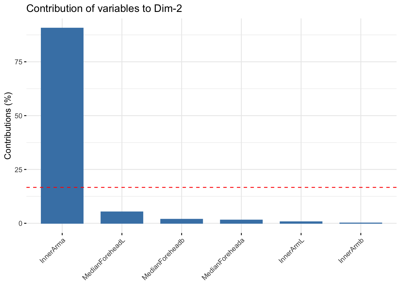

Past versions of winterciecomps-3.png

Version	Author	Date
d9fb6da	Lily Heald	2025-02-04

summer_cie_scale <- scale(summer_cie)
summer_cie_pca <- prcomp(summer_cie_scale)
summary(summer_cie_pca)

Importance of components:
                          PC1    PC2     PC3    PC4     PC5     PC6
Standard deviation     2.0738 0.9392 0.64280 0.4960 0.32130 0.23426
Proportion of Variance 0.7168 0.1470 0.06886 0.0410 0.01721 0.00915
Cumulative Proportion  0.7168 0.8638 0.93265 0.9737 0.99085 1.00000

summer_cie_pca$loadings[, 1:2]

NULL

fviz_eig(summer_cie_pca, addlabels = TRUE)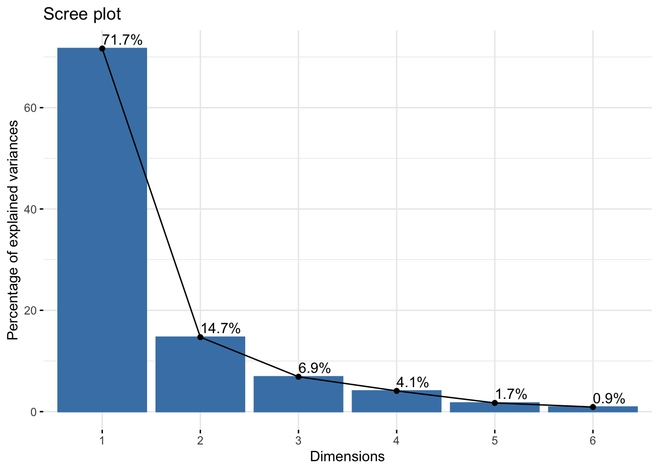

Past versions of summerciepca-1.png

Version	Author	Date
d9fb6da	Lily Heald	2025-02-04

fviz_pca_var(summer_cie_pca, col.var = "black")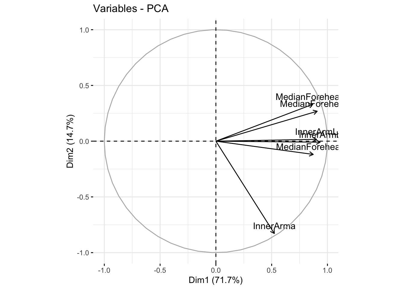

Past versions of summerciepca-2.png

Version	Author	Date
d9fb6da	Lily Heald	2025-02-04

fviz_cos2(summer_cie_pca, choice = "var", axes = 1:2)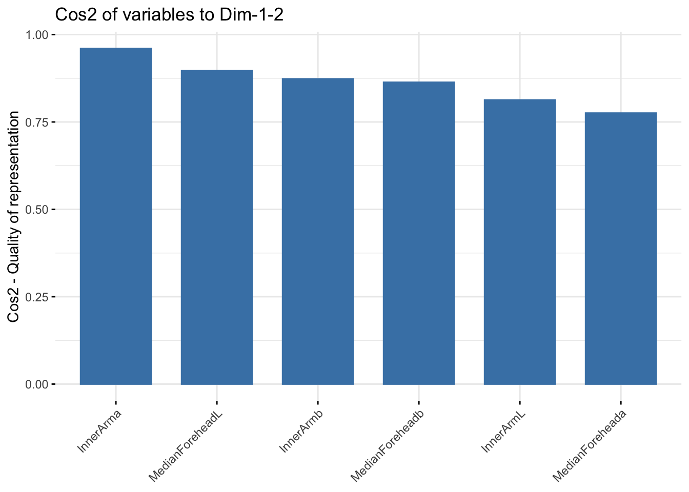

Past versions of summerciepca-3.png

Version	Author	Date
d9fb6da	Lily Heald	2025-02-04

summer_cie_comps <- as.data.frame(summer_cie_pca$x)
summer_cie_new <- cbind(summer_data,summer_cie_comps[,c(1,2)])

ggplot(summer_cie_new, aes(x=PC1, y=PC2, col = Ethnicity, fill = Ethnicity)) +
  stat_ellipse(geom = "polygon", col= "black", alpha =0.5)+
  geom_point(shape=21, col="black") +
  labs(title = "Summer CIELAB PCA")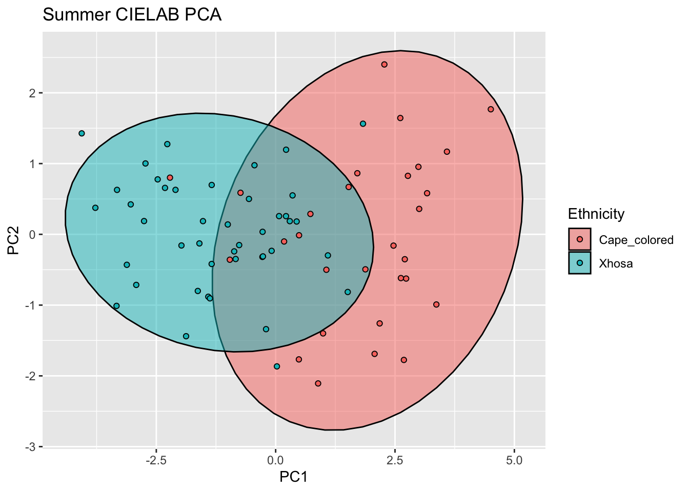

Past versions of summerciecomps-1.png

Version	Author	Date
d9fb6da	Lily Heald	2025-02-04

fviz_contrib(summer_cie_pca, choice = "var", axes = 1, top = 10)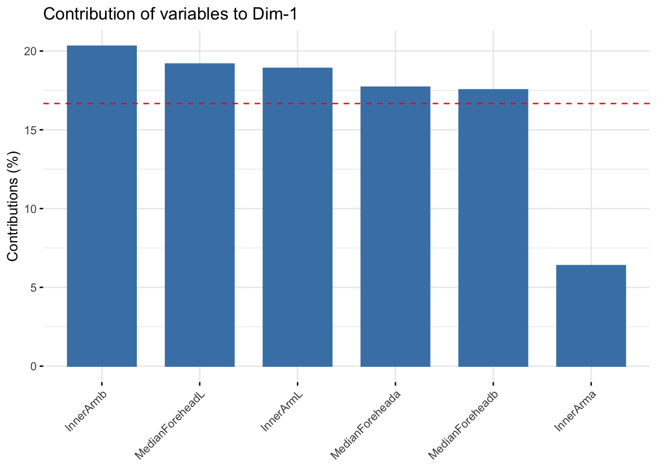

Past versions of summerciecomps-2.png

Version	Author	Date
d9fb6da	Lily Heald	2025-02-04

fviz_contrib(summer_cie_pca, choice = "var", axes = 2, top = 10)

Past versions of summerciecomps-3.png

Version	Author	Date
d9fb6da	Lily Heald	2025-02-04

six_cie_scale <- scale(six_cie)
six_cie_pca <- prcomp(six_cie_scale)
summary(six_cie_pca)

Importance of components:
                          PC1    PC2     PC3     PC4     PC5     PC6
Standard deviation     1.9741 1.1342 0.62622 0.54034 0.27271 0.24039
Proportion of Variance 0.6495 0.2144 0.06536 0.04866 0.01239 0.00963
Cumulative Proportion  0.6495 0.8639 0.92931 0.97797 0.99037 1.00000

six_cie_pca$loadings[, 1:2]

NULL

fviz_eig(six_cie_pca, addlabels = TRUE)

Past versions of sixciepca-1.png

Version	Author	Date
d9fb6da	Lily Heald	2025-02-04

fviz_pca_var(six_cie_pca, col.var = "black")

Past versions of sixciepca-2.png

Version	Author	Date
d9fb6da	Lily Heald	2025-02-04

fviz_cos2(six_cie_pca, choice = "var", axes = 1:2)

Past versions of sixciepca-3.png

Version	Author	Date
d9fb6da	Lily Heald	2025-02-04

six_cie_comps <- as.data.frame(six_cie_pca$x)
six_cie_new <- cbind(six_week_data,six_cie_comps[,c(1,2)])

ggplot(six_rgb_new, aes(x=PC1, y=PC2, col = Ethnicity, fill = Ethnicity)) +
  stat_ellipse(geom = "polygon", col= "black", alpha =0.5)+
  geom_point(shape=21, col="black") +
  labs(title = "Six Week CIELAB PCA")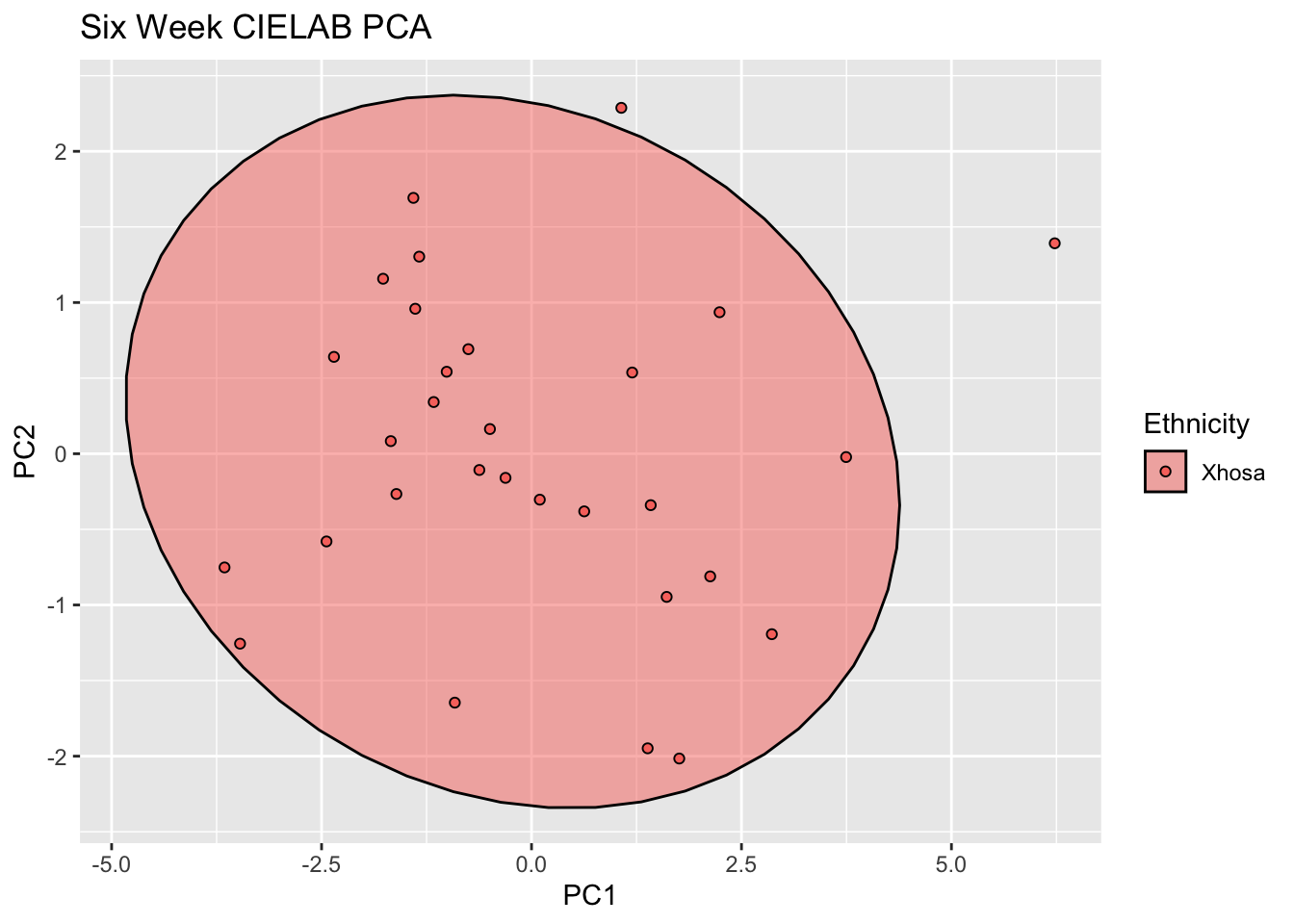

Past versions of sixciecomps-1.png

Version	Author	Date
d9fb6da	Lily Heald	2025-02-04

fviz_contrib(six_cie_pca, choice = "var", axes = 1, top = 10)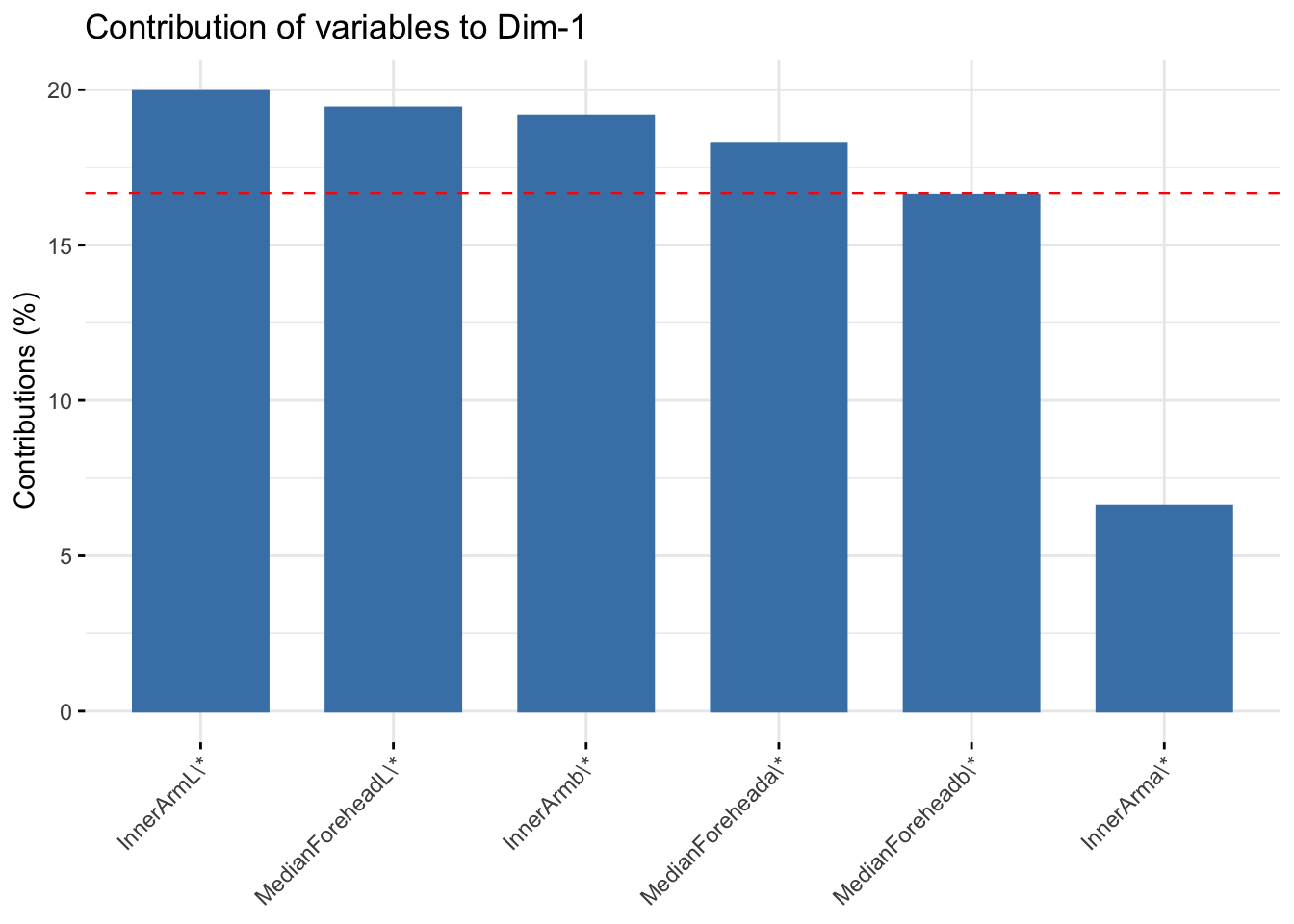

Past versions of sixciecomps-2.png

Version	Author	Date
d9fb6da	Lily Heald	2025-02-04

fviz_contrib(six_cie_pca, choice = "var", axes = 2, top = 10)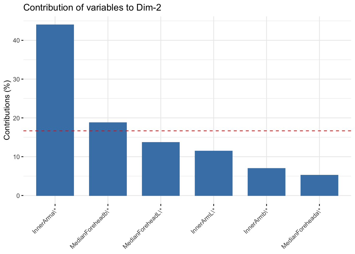

Past versions of sixciecomps-3.png

Version	Author	Date
d9fb6da	Lily Heald	2025-02-04

part 2: visualizations

joined_data <- joined_data %>%
  select(matches("Participant|Ethnicity_|InnerArm|MedianForehead|VitD|Diff"))
long_data <- joined_data %>%
  pivot_longer(
    cols = -ParticipantCentreID,  
    names_to = c(".value", "Season"),        # Split column names into two parts
    names_sep = "_"                          # Separate at _
  )

ggplot(long_data, aes(x = MedianForeheadM, fill = Ethnicity)) +
  geom_histogram(alpha = 0.5, position = "identity") 

`stat_bin()` using `bins = 30`. Pick better value with `binwidth`.

Warning: Removed 68 rows containing non-finite outside the scale range
(`stat_bin()`).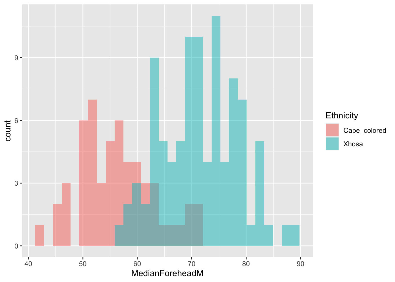

Past versions of histogram-1.png

Version	Author	Date
d9fb6da	Lily Heald	2025-02-04

cape_colored <- long_data[long_data$Ethnicity == "Cape_colored",]
ggplot(cape_colored, aes(x = MedianForeheadM, fill = ..x..)) +
  geom_histogram() +
  scale_fill_gradient(low="#D2B48C", high="#1B0000") + 
  theme_minimal() +
  labs(
    title = "Distribution of Forehead Melanin Index by Ethnicity ~ Cape_colored",
    x = "Forehead Melanin Index",
    y = "Count"
  )

Warning: The dot-dot notation (`..x..`) was deprecated in ggplot2 3.4.0.
ℹ Please use `after_stat(x)` instead.
This warning is displayed once every 8 hours.
Call `lifecycle::last_lifecycle_warnings()` to see where this warning was
generated.

`stat_bin()` using `bins = 30`. Pick better value with `binwidth`.

Warning: Removed 68 rows containing non-finite outside the scale range
(`stat_bin()`).

Past versions of histogram-2.png

Version	Author	Date
d9fb6da	Lily Heald	2025-02-04

xhosa <- long_data[long_data$Ethnicity == "Xhosa",]
ggplot(xhosa, aes(x = MedianForeheadM, fill = ..x..)) +
  geom_histogram() +
  scale_fill_gradient(low="#D2B48C", high="#1B0000") + 
  theme_minimal() +
  labs(
    title = "Distribution of Forehead Melanin Index by Ethnicity ~ Xhosa",
    x = "Forehead Melanin Index",
    y = "Count"
  )

`stat_bin()` using `bins = 30`. Pick better value with `binwidth`.

Warning: Removed 68 rows containing non-finite outside the scale range
(`stat_bin()`).

Past versions of histogram-3.png

Version	Author	Date
d9fb6da	Lily Heald	2025-02-04

filtered_data <- long_data %>%
  filter(!is.na(Ethnicity))
ggplot(filtered_data, aes(x = MedianForeheadM, fill = ..x..)) +
  geom_histogram() +
  facet_grid(Ethnicity ~ .) +
  scale_fill_gradient(
    low = "#D2B48C", # Light tan
    high = "#1B0000" # Dark brown
  ) +
  theme_minimal() +
  labs(
    title = "Distribution of Forehead Melanin Index by Ethnicity",
    x = "Forehead Melanin Index",
    y = "Count",
    fill = "Melanin Index"
  )

`stat_bin()` using `bins = 30`. Pick better value with `binwidth`.

Past versions of histogram-4.png

Version	Author	Date
d9fb6da	Lily Heald	2025-02-04

filtered_data <- long_data %>%
  filter(!is.na(Ethnicity))
ggplot(filtered_data, aes(x = MedianForeheadM, fill = ..x..)) +
  geom_histogram() +
  facet_grid(Ethnicity ~ Season) +
  scale_fill_gradient(
    low = "#D2B48C", # Light tan
    high = "#1B0000" # Dark brown
  ) +
  theme_minimal() +
  labs(
    title = "Distribution of Forehead Melanin Index by Ethnicity",
    x = "Forehead Melanin Index",
    y = "Count",
    fill = "Melanin Index"
  )

`stat_bin()` using `bins = 30`. Pick better value with `binwidth`.

Past versions of histogram-5.png

Version	Author	Date
d9fb6da	Lily Heald	2025-02-04

xhosa <- xhosa %>%
  filter(!is.na(Ethnicity)) %>%
  filter(!is.na(Season))
xhosa %>%
  group_by(Season) %>%
  shapiro_test(InnerArmM)

# A tibble: 3 × 4
  Season   variable  statistic     p
  <chr>    <chr>         <dbl> <dbl>
1 sixweeks InnerArmM     0.954 0.337
2 summer   InnerArmM     0.977 0.520
3 winter   InnerArmM     0.952 0.239

# xhosa is normally distributed in each season (p>0.05)

cape_colored <- cape_colored %>%
  filter(!is.na(Ethnicity)) %>%
  filter(!is.na(Season))
cape_colored %>%
  group_by(Season) %>%
  shapiro_test(InnerArmM)

# A tibble: 2 × 4
  Season variable  statistic       p
  <chr>  <chr>         <dbl>   <dbl>
1 summer InnerArmM     0.895 0.00727
2 winter InnerArmM     0.873 0.00509

# cape_colored is not normally distributed in each season (p<0.05)

ggqqplot(cape_colored, "InnerArmM", facet.by = "Season")

Past versions of constitutive_hypothesis-1.png

Version	Author	Date
d9fb6da	Lily Heald	2025-02-04

ggqqplot(xhosa, "InnerArmM", facet.by = "Season")

Past versions of constitutive_hypothesis-2.png

Version	Author	Date
d9fb6da	Lily Heald	2025-02-04

aov_result_x <- aov(InnerArmM ~ Season, data = xhosa)

broom::tidy(aov_result_x)

# A tibble: 2 × 6
  term         df  sumsq meansq statistic p.value
  <chr>     <dbl>  <dbl>  <dbl>     <dbl>   <dbl>
1 Season        2   29.8   14.9     0.560   0.573
2 Residuals    91 2420.    26.6    NA      NA    

# filtered_data <- long_data %>%
#   filter(!is.na(Ethnicity))
# ggplot(filtered_data, aes(x = MDifference)) +
#   geom_histogram() +
#   facet_grid(Ethnicity ~ Season) +
#   theme_minimal() +
#   labs(
#     title = "Difference in Forehead and Inner Arm Melanin Index by Ethnicity and Season",
#     x = "Difference in Forehead MI and Inner Arm MI",
#     y = "Count",
#   )
# 
# filtered_data <- long_data %>%
#   filter(!is.na(Ethnicity))
# ggplot(filtered_data, aes(x = Ethnicity, y = MDifference)) +
#   geom_boxplot() +
#   facet_grid(.~Season) +
#   theme_minimal() +
#   labs(
#     title = "Difference in Forehead and Inner Arm Melanin Index by Ethnicity and Season",
#     x = "Difference in Forehead MI and Inner Arm MI",
#     y = "Count"
#   )

summer_data$Ethnicity <- as.factor (summer_data$Ethnicity) 
names(summer_data) <- gsub("\\\\", "", names(summer_data))
names(summer_data) <- gsub("\\*", "", names(summer_data))
#Xhosa is value 2
winter_data$Ethnicity <- as.factor (winter_data$Ethnicity) 
names(winter_data) <- gsub("\\\\", "", names(winter_data))
names(winter_data) <- gsub("\\*", "", names(winter_data))
# cielab colorspaces different between groups
lstarresult <- t.test(MedianForeheadL ~ Ethnicity, data = summer_data)
lstarp_value <- lstarresult$p.value
ggplot(summer_data, aes(x = Ethnicity, y = MedianForeheadL, fill = Ethnicity)) +
  geom_boxplot() +
  annotate("text", x = 1.5, y = max(summer_data$MedianForeheadL), 
           label = paste("p =", signif(lstarp_value, digits = 3)), 
           size = 5) +
  labs(title = "summer L star")

Past versions of t-tests-1.png

Version	Author	Date
d9fb6da	Lily Heald	2025-02-04

astarresult <- t.test(MedianForeheada ~ Ethnicity, data = summer_data)
astarp_value <- astarresult$p.value
ggplot(summer_data, aes(x = Ethnicity, y = MedianForeheada, fill = Ethnicity)) +
  geom_boxplot() +
  annotate("text", x = 1.5, y = max(summer_data$MedianForeheada), 
           label = paste("p =", signif(astarp_value, digits = 3)), 
           size = 5) +
  labs(title = "summer a star")

Past versions of t-tests-2.png

Version	Author	Date
d9fb6da	Lily Heald	2025-02-04

bstarresult <- t.test(MedianForeheadb ~ Ethnicity, data = summer_data)
bstarp_value <- bstarresult$p.value
ggplot(summer_data, aes(x = Ethnicity, y = MedianForeheadb, fill = Ethnicity)) +
  geom_boxplot() +
  annotate("text", x = 1.5, y = max(summer_data$MedianForeheadb), 
           label = paste("p =", signif(bstarp_value, digits = 3)), 
           size = 5) +
  labs(title = "summer b star")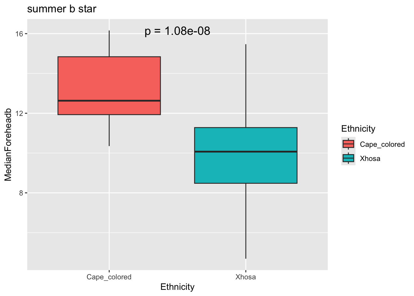

Past versions of t-tests-3.png

Version	Author	Date
d9fb6da	Lily Heald	2025-02-04

winter versus summer t test across all colors

# ME colorspaces different between groups
Mresult <- t.test(MedianForeheadM ~ Ethnicity, data = summer_data)
Mp_value <- Mresult$p.value
ggplot(summer_data, aes(x = Ethnicity, y = MedianForeheadM, fill = Ethnicity)) +
  geom_boxplot() +
  annotate("text", x = 1.5, y = max(summer_data$MedianForeheadM), 
           label = paste("p =", signif(Mp_value, digits = 3)), 
           size = 5) +
  labs(title = "Summer Melanin")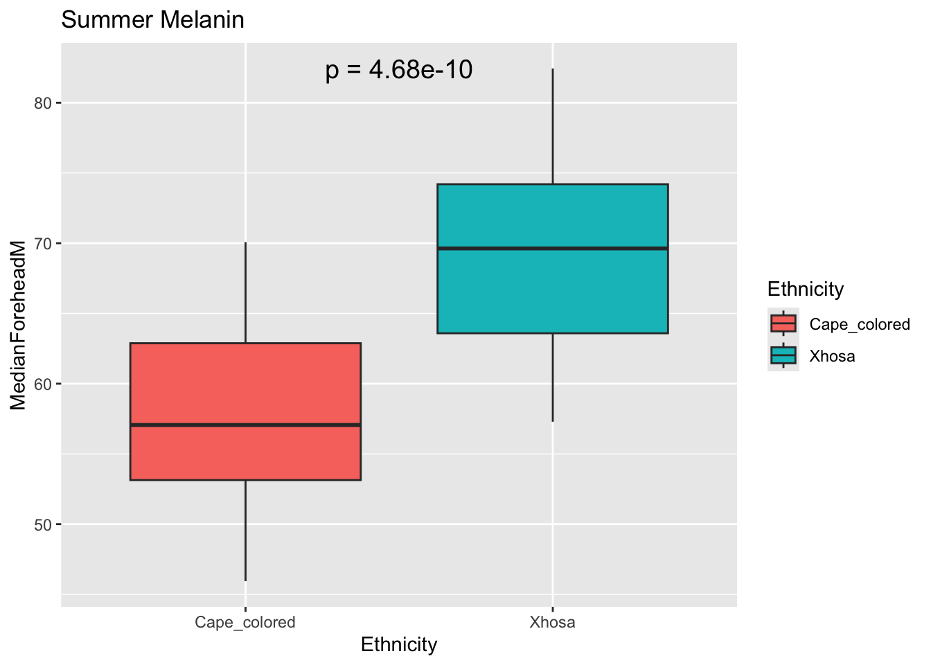

Past versions of metest-1.png

Version	Author	Date
d9fb6da	Lily Heald	2025-02-04

Eresult <- t.test(MedianForeheadE ~ Ethnicity, data = summer_data)
Ep_value <- Eresult$p.value
ggplot(summer_data, aes(x = Ethnicity, y = MedianForeheadE, fill = Ethnicity)) +
  geom_boxplot() +
  annotate("text", x = 1.5, y = max(summer_data$MedianForeheadE), 
           label = paste("p =", signif(Ep_value, digits = 3)), 
           size = 5) +
  labs(title = "Summer Erythema")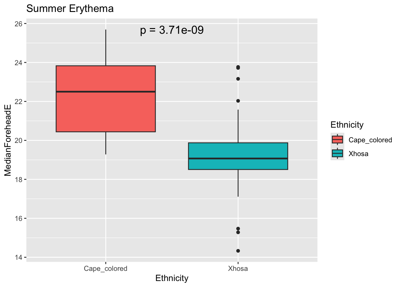

Past versions of metest-2.png

Version	Author	Date
d9fb6da	Lily Heald	2025-02-04

Mresult <- t.test(MedianForeheadM ~ Ethnicity, data = winter_data)
Mp_value <- Mresult$p.value
ggplot(winter_data, aes(x = Ethnicity, y = MedianForeheadM, fill = Ethnicity)) +
  geom_boxplot() +
  annotate("text", x = 1.5, y = max(winter_data$MedianForeheadM), 
           label = paste("p =", signif(Mp_value, digits = 3)), 
           size = 5) +
  labs(title = "Winter Melanin")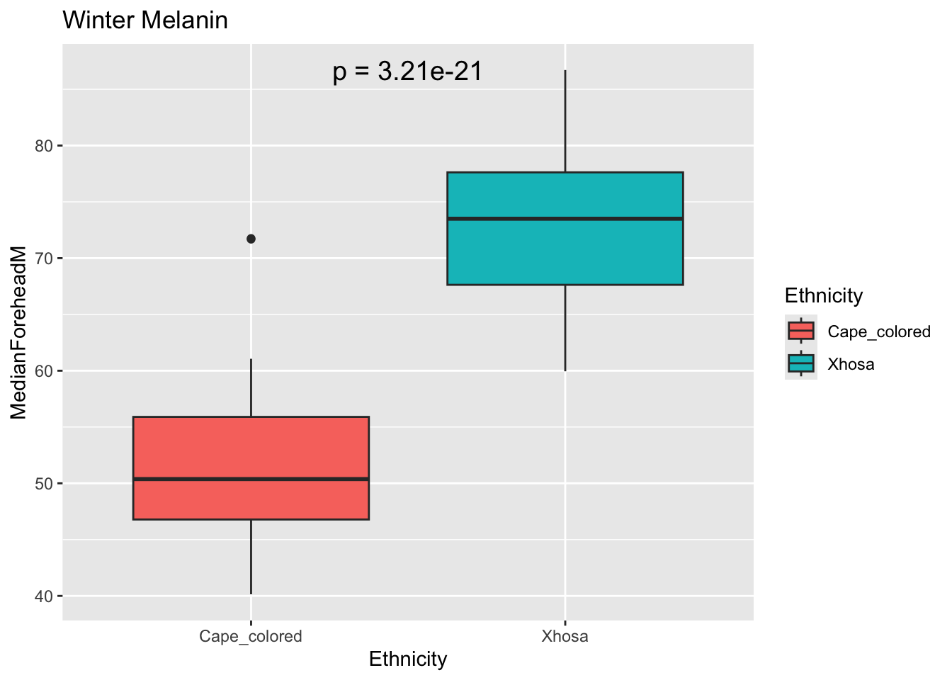

Past versions of metest-3.png

Version	Author	Date
d9fb6da	Lily Heald	2025-02-04

Eresult <- t.test(MedianForeheadE ~ Ethnicity, data = winter_data)
Ep_value <- Eresult$p.value
ggplot(winter_data, aes(x = Ethnicity, y = MedianForeheadE, fill = Ethnicity)) +
  geom_boxplot() +
  annotate("text", x = 1.5, y = max(winter_data$MedianForeheadE), 
           label = paste("p =", signif(Ep_value, digits = 3)), 
           size = 5) +
  labs(title = "Winter Erythema")

Past versions of metest-4.png

Version	Author	Date
d9fb6da	Lily Heald	2025-02-04

# RGB colorspaces different between groups
Rresult <- t.test(MedianForeheadR ~ Ethnicity, data = winter_data)
Rp_value <- Rresult$p.value
ggplot(winter_data, aes(x = Ethnicity, y = MedianForeheadR, fill = Ethnicity)) +
  geom_boxplot() +
  annotate("text", x = 1.5, y = max(winter_data$MedianForeheadR), 
           label = paste("p =", signif(Rp_value, digits = 3)), 
           size = 5) +
  labs(title = "Winter R")

Past versions of rgbtest-1.png

Version	Author	Date
d9fb6da	Lily Heald	2025-02-04

winterB <- t.test(MedianForeheadB ~ Ethnicity, data = winter_data)
winterBp <- winterB$p.value
ggplot(winter_data, aes(x = Ethnicity, y = MedianForeheadB, fill = Ethnicity)) +
  geom_boxplot() +
  annotate("text", x = 1.5, y = max(winter_data$MedianForeheadB), 
           label = paste("p =", signif(winterBp, digits = 3)), 
           size = 5) +
  labs(title = "Winter B")

Past versions of rgbtest-2.png

Version	Author	Date
d9fb6da	Lily Heald	2025-02-04

winterG <- t.test(MedianForeheadG ~ Ethnicity, data = winter_data)
winterGp <- winterG$p.value
ggplot(winter_data, aes(x = Ethnicity, y = MedianForeheadG, fill = Ethnicity)) +
  geom_boxplot() +
  annotate("text", x = 1.5, y = max(winter_data$MedianForeheadG), 
           label = paste("p =", signif(winterGp, digits = 3)), 
           size = 5) +
  labs(title = "Winter G")

Past versions of rgbtest-3.png

Version	Author	Date
d9fb6da	Lily Heald	2025-02-04

Session information

sessionInfo()

R version 4.4.2 (2024-10-31)
Platform: aarch64-apple-darwin20
Running under: macOS Monterey 12.5.1

Matrix products: default
BLAS:   /Library/Frameworks/R.framework/Versions/4.4-arm64/Resources/lib/libRblas.0.dylib 
LAPACK: /Library/Frameworks/R.framework/Versions/4.4-arm64/Resources/lib/libRlapack.dylib;  LAPACK version 3.12.0

locale:
[1] en_US.UTF-8/en_US.UTF-8/en_US.UTF-8/C/en_US.UTF-8/en_US.UTF-8

time zone: America/Detroit
tzcode source: internal

attached base packages:
[1] stats     graphics  grDevices utils     datasets  methods   base     

other attached packages:
 [1] lme4_1.1-36        Matrix_1.7-1       rstatix_0.7.2      ggpubr_0.6.0      
 [5] ggfortify_0.4.17   wesanderson_0.3.7  missMDA_1.19       FactoMineR_2.11   
 [9] factoextra_1.0.7   ggcorrplot_0.1.4.1 corrr_0.4.4        readxl_1.4.3      
[13] lubridate_1.9.4    forcats_1.0.0      stringr_1.5.1      purrr_1.0.2       
[17] tibble_3.2.1       ggplot2_3.5.1      tidyverse_2.0.0    tidyr_1.3.1       
[21] dplyr_1.1.4        readr_2.1.5        workflowr_1.7.1   

loaded via a namespace (and not attached):
  [1] Rdpack_2.6.2         gridExtra_2.3        sandwich_3.1-1      
  [4] rlang_1.1.4          magrittr_2.0.3       git2r_0.35.0        
  [7] multcomp_1.4-28      compiler_4.4.2       getPass_0.2-4       
 [10] callr_3.7.6          vctrs_0.6.5          crayon_1.5.3        
 [13] pkgconfig_2.0.3      shape_1.4.6.1        fastmap_1.2.0       
 [16] backports_1.5.0      labeling_0.4.3       utf8_1.2.4          
 [19] promises_1.3.2       rmarkdown_2.29       tzdb_0.4.0          
 [22] nloptr_2.1.1         ps_1.8.1             xfun_0.50           
 [25] glmnet_4.1-8         jomo_2.7-6           cachem_1.1.0        
 [28] jsonlite_1.8.9       flashClust_1.01-2    later_1.4.1         
 [31] pan_1.9              broom_1.0.7          parallel_4.4.2      
 [34] cluster_2.1.8        R6_2.5.1             bslib_0.8.0         
 [37] stringi_1.8.4        car_3.1-3            rpart_4.1.24        
 [40] boot_1.3-31          jquerylib_0.1.4      cellranger_1.1.0    
 [43] estimability_1.5.1   Rcpp_1.0.14          iterators_1.0.14    
 [46] knitr_1.49           zoo_1.8-12           nnet_7.3-20         
 [49] httpuv_1.6.15        splines_4.4.2        timechange_0.3.0    
 [52] tidyselect_1.2.1     abind_1.4-8          rstudioapi_0.17.1   
 [55] yaml_2.3.10          doParallel_1.0.17    codetools_0.2-20    
 [58] processx_3.8.5       lattice_0.22-6       withr_3.0.2         
 [61] coda_0.19-4.1        evaluate_1.0.3       survival_3.8-3      
 [64] pillar_1.10.1        carData_3.0-5        mice_3.17.0         
 [67] whisker_0.4.1        DT_0.33              foreach_1.5.2       
 [70] reformulas_0.4.0     generics_0.1.3       rprojroot_2.0.4     
 [73] hms_1.1.3            munsell_0.5.1        scales_1.3.0        
 [76] minqa_1.2.8          xtable_1.8-4         leaps_3.2           
 [79] glue_1.8.0           emmeans_1.10.6       scatterplot3d_0.3-44
 [82] tools_4.4.2          ggsignif_0.6.4       fs_1.6.5            
 [85] mvtnorm_1.3-3        grid_4.4.2           rbibutils_2.3       
 [88] colorspace_2.1-1     nlme_3.1-166         Formula_1.2-5       
 [91] cli_3.6.3            gtable_0.3.6         sass_0.4.9          
 [94] digest_0.6.37        ggrepel_0.9.6        TH.data_1.1-3       
 [97] farver_2.1.2         htmlwidgets_1.6.4    htmltools_0.5.8.1   
[100] lifecycle_1.0.4      httr_1.4.7           multcompView_0.1-10 
[103] mitml_0.4-5          MASS_7.3-64