statsplot

workflowr

• Summary
• Checks
• Past versions

Last updated: 2025-02-04

Checks: 6 1

Knit directory: sapphire/

This reproducible R Markdown analysis was created with workflowr (version 1.7.1). The Checks tab describes the reproducibility checks that were applied when the results were created. The Past versions tab lists the development history.

---

R Markdown file: up-to-date

Great! Since the R Markdown file has been committed to the Git repository, you know the exact version of the code that produced these results.

Environment: empty

Great job! The global environment was empty. Objects defined in the global environment can affect the analysis in your R Markdown file in unknown ways. For reproduciblity it’s best to always run the code in an empty environment.

Seed: set.seed(20240923)

The command set.seed(20240923) was run prior to running the code in the R Markdown file. Setting a seed ensures that any results that rely on randomness, e.g. subsampling or permutations, are reproducible.

Session information: recorded

Great job! Recording the operating system, R version, and package versions is critical for reproducibility.

Cache: none

Nice! There were no cached chunks for this analysis, so you can be confident that you successfully produced the results during this run.

File paths: absolute

Using absolute paths to the files within your workflowr project makes it difficult for you and others to run your code on a different machine. Change the absolute path(s) below to the suggested relative path(s) to make your code more reproducible.

absolute	relative
~/sapphire/data/serum_vit_D_study_with_lab_results.xlsx	data/serum_vit_D_study_with_lab_results.xlsx
~/sapphire/data/sun_expos_data/sun_expos_long.csv	data/sun_expos_data/sun_expos_long.csv
~/sapphire/data/summer_winter.csv	data/summer_winter.csv
~/sapphire/SAfrADMIX/long.csv	SAfrADMIX/long.csv

Repository version: 5636f2f

Great! You are using Git for version control. Tracking code development and connecting the code version to the results is critical for reproducibility.

The results in this page were generated with repository version 5636f2f. See the Past versions tab to see a history of the changes made to the R Markdown and HTML files.

Note that you need to be careful to ensure that all relevant files for the analysis have been committed to Git prior to generating the results (you can use wflow_publish or wflow_git_commit). workflowr only checks the R Markdown file, but you know if there are other scripts or data files that it depends on. Below is the status of the Git repository when the results were generated:

Ignored files:
    Ignored:    .DS_Store
    Ignored:    .RData
    Ignored:    .Rhistory
    Ignored:    .Rproj.user/
    Ignored:    analysis/.RData
    Ignored:    analysis/.Rhistory

Untracked files:
    Untracked:  .lock_gPLINK
    Untracked:  .metafile_gPLINK
    Untracked:  SAfrADMIX/
    Untracked:  analysis/genotype.R
    Untracked:  analysis/lilyanalysis.Rmd
    Untracked:  data/dist_pops.csv
    Untracked:  data/summer_winter.csv

Note that any generated files, e.g. HTML, png, CSS, etc., are not included in this status report because it is ok for generated content to have uncommitted changes.

---

These are the previous versions of the repository in which changes were made to the R Markdown (analysis/statsplot.Rmd) and HTML (docs/statsplot.html) files. If you’ve configured a remote Git repository (see ?wflow_git_remote), click on the hyperlinks in the table below to view the files as they were in that past version.

File	Version	Author	Date	Message
Rmd	d9fb6da	Lily Heald	2025-02-04	wflow
html	d9fb6da	Lily Heald	2025-02-04	wflow
Rmd	ce202c9	Lily Heald	2025-02-04	create statsplot.Rmd

---

file_path <- "~/sapphire/data/serum_vit_D_study_with_lab_results.xlsx" 
data_summer <- read_excel(file_path, sheet = "ScreeningDataCollectionSummer")
data_winter <- read_excel(file_path, sheet = "ScreeningDataCollectionWinter")
data_6weeks <- read_excel(file_path, sheet = "ScreeningDataCollection6Weeks")
sun_expos <- read.csv("~/sapphire/data/sun_expos_data/sun_expos_long.csv")
sun_expos_summer <- sun_expos[sun_expos$collection_period == 'Summer', ]
sun_expos_winter <- sun_expos[sun_expos$collection_period == 'Winter', ]
sun_expos_6Weeks <- sun_expos[sun_expos$collection_period == '6Weeks', ]
summer_winter <- read.csv("~/sapphire/data/summer_winter.csv")

long_data <- summer_winter %>%
  pivot_longer(
    cols = -ParticipantCentreID,  
    names_to = c(".value", "Season"),  # Extract variable name and season
    names_sep = "_"                    # Separate at "_"
  )

numpairs <- long_data %>%
  filter(!is.na(MedianForeheadM)) %>%
  group_by(ParticipantCentreID) %>%
  filter(all(c('summer', 'winter') %in% Season)) %>%
  summarise(count = n_distinct(ParticipantCentreID))

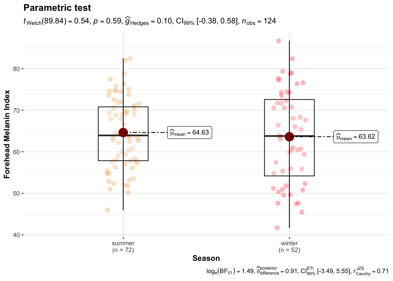
write.csv(long_data, "~/sapphire/SAfrADMIX/long.csv", row.names = F)

ggbetweenstats(
  data = long_data,
  x = Season,
  y = MedianForeheadM,
  xlab ="Season",
  ylab = "Forehead Melanin Index",
  violin.args = list(width = 0),
  type = "p",
  conf.level = 0.99,
  title = "Parametric test",
  package = "wesanderson",
  palette = "GrandBudapest1"
)

Past versions of unnamed-chunk-1-1.png

Version	Author	Date
d9fb6da	Lily Heald	2025-02-04

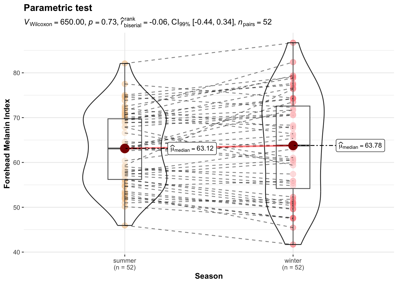
ggwithinstats(
  data = long_data,
  x = Season,
  y = MedianForeheadM,
  xlab ="Season",
  ylab = "Forehead Melanin Index",
  type = "np",
  conf.level = 0.99,
  title = "Parametric test",
  package = "wesanderson",
  palette = "GrandBudapest1"
)

Past versions of unnamed-chunk-2-1.png

Version	Author	Date
d9fb6da	Lily Heald	2025-02-04

Goal: winter versus summer t test across all colors

# p1 <- ggwithinstats(
#   data = long_data,
#   x = Season,
#   y = MedianForeheadM,
#   type = "p",
#   effsize.type = "d",
#   conf.level = 0.99,
#   title = "Parametric test",
#   package = "ggsci",
#   palette = "nrc_npg"
# )

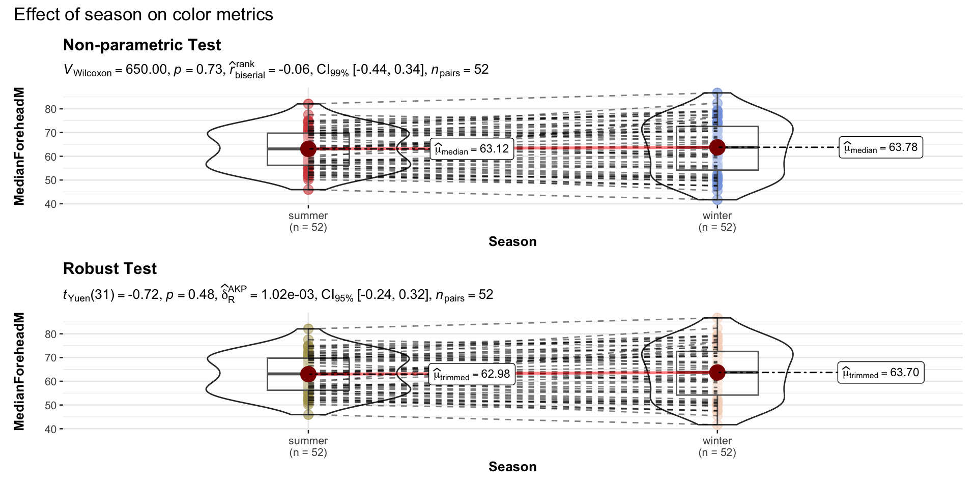
## Mann-Whitney U test (nonparametric test)
p2 <- ggwithinstats(
  data = long_data,
  x = Season,
  y = MedianForeheadM,
  xlab = "Season",
  ylab = "MedianForeheadM
  ",
  type = "np",
  conf.level = 0.99,
  title = "Non-parametric Test",
  package = "ggsci",
  palette = "uniform_startrek"
)

## robust t-test
p3 <- ggwithinstats(
  data = long_data,
  x = Season,
  y = MedianForeheadM,
  xlab = "Season",
  ylab = "MedianForeheadM",
  type = "r",
  conf.level = 0.99,
  title = "Robust Test",
  package = "wesanderson",
  palette = "Royal2"
)

## Bayes Factor for parametric t-test
# p4 <- ggwithinstats(
#   data = long_data,
#   x = Season,
#   y = MedianForeheadM,
#   xlab = "Season",
#   ylab = "MedianForeheadM",
#   type = "bayes",
#   title = "Bayesian Test",
#   package = "ggsci",
#   palette = "nrc_npg"
# )

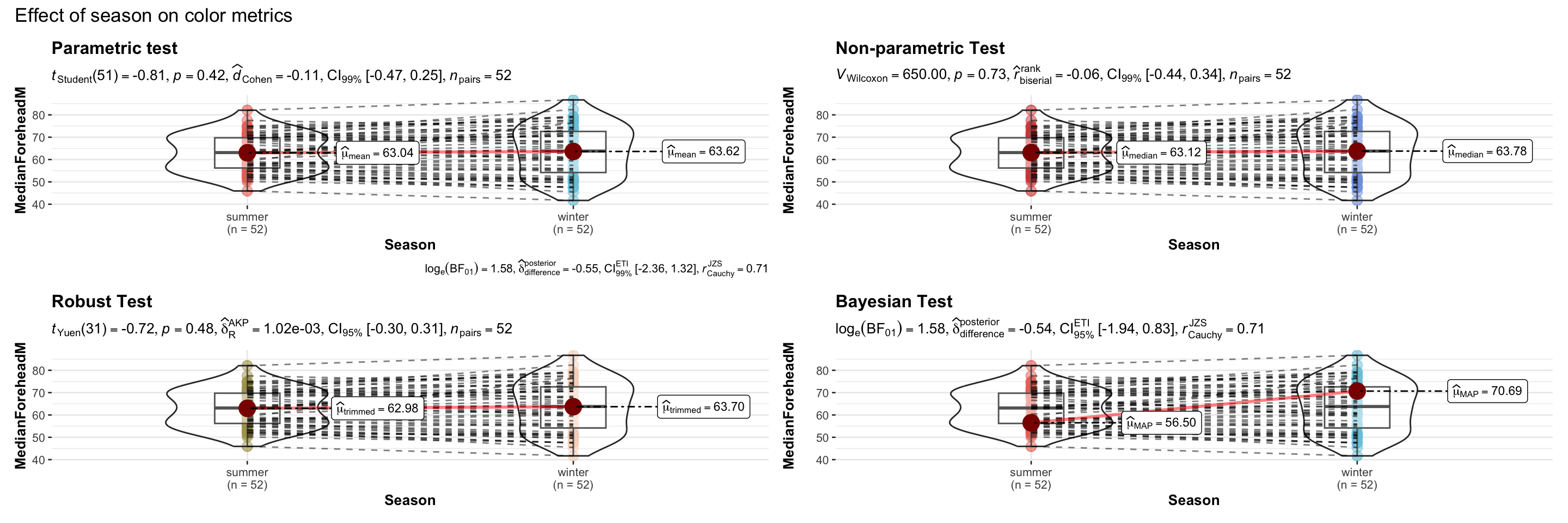
# combining the individual plots into a single plot
combine_plots(
  plotlist = list(p2, p3),
  plotgrid.args = list(nrow = 2),
  annotation.args = list(
    title = "Effect of season on color metrics"),
  height = 10,  # Increase the height (adjust as needed)
  width = 12 
)

Past versions of unnamed-chunk-3-1.png

Version	Author	Date
d9fb6da	Lily Heald	2025-02-04

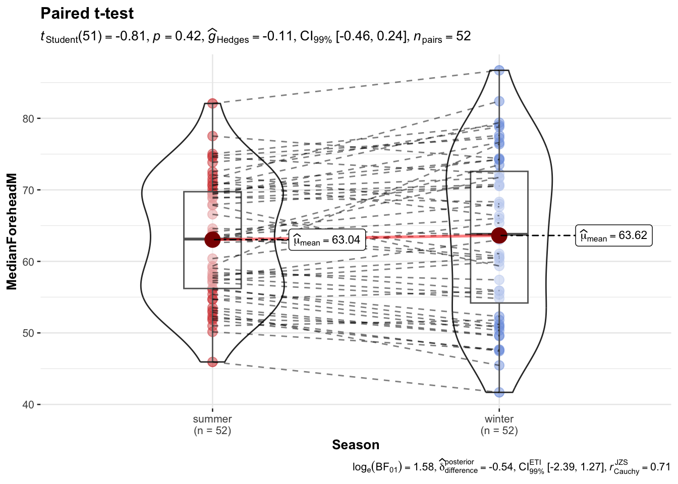
library(ggstatsplot)

ggwithinstats(
  data   = long_data,
  x      = Season,
  y      = MedianForeheadM,
  paired = TRUE,                     # must be TRUE for repeated measures
  id     = "ParticipantCentreID",    # ID column to match pairs
  type   = "parametric",             # paired t-test
  conf.level = 0.99,
  title     = "Paired t-test",
  xlab      = "Season",
  ylab      = "MedianForeheadM",
  package   = "ggsci",
  palette   = "uniform_startrek"
)

Past versions of unnamed-chunk-4-1.png

Version	Author	Date
d9fb6da	Lily Heald	2025-02-04

p1 <- ggwithinstats(
  data = long_data,
  x = Season,
  y = MedianForeheadM,
  xlab = "Season",
  ylab = "MedianForeheadM",
  type = "r",
  title = "Robust Test",
  package = "wesanderson",
  palette = "Royal2", 
  centrality.label.args = list(size  = 5)
)

p2 <- ggwithinstats(
  data = long_data,
  x = Season,
  y = MedianForeheadE,
  xlab = "Season",
  ylab = "MedianForeheadE",
  type = "r",
  title = "Robust Test",
  package = "wesanderson",
  palette = "Royal2",
  centrality.label.args = list(size  = 5)
)

p3 <- ggwithinstats(
  data = long_data,
  x = Season,
  y = MedianForeheadL,
  xlab = "Season",
  ylab = "MedianForeheadL",
  type = "r",
  title = "Robust Test",
  package = "wesanderson",
  palette = "Royal2",
  centrality.label.args = list(size  = 5)
)

p4 <- ggwithinstats(
  data = long_data,
  x = Season,
  y = MedianForeheada,
  xlab = "Season",
  ylab = "MedianForeheada",
  type = "r",
  title = "Robust Test",
  package = "wesanderson",
  palette = "Royal2", 
  centrality.label.args = list(size  = 5)
)

p5 <- ggwithinstats(
  data = long_data,
  x = Season,
  y = MedianForeheadb,
  xlab = "Season",
  ylab = "MedianForeheadb",
  type = "r",
  title = "Robust Test",
  package = "wesanderson",
  palette = "Royal2",
  centrality.label.args = list(size  = 5)
)

p6 <- ggwithinstats(
  data = long_data,
  x = Season,
  y = MedianForeheadR,
  xlab = "Season",
  ylab = "MedianForeheadR",
  type = "r",
  title = "Robust Test",
  package = "wesanderson",
  palette = "Royal2",
  centrality.label.args = list(size  = 5)
)

p7 <- ggwithinstats(
  data = long_data,
  x = Season,
  y = MedianForeheadG,
  xlab = "Season",
  ylab = "MedianForeheadG",
  type = "r",
  title = "Robust Test",
  package = "wesanderson",
  palette = "Royal2",
  centrality.label.args = list(size  = 5)
)

p8 <- ggwithinstats(
  data = long_data,
  x = Season,
  y = MedianForeheadB,
  xlab = "Season",
  ylab = "MedianForeheadB",
  type = "r",
  title = "Robust Test",
  package = "wesanderson",
  palette = "Royal2",
  centrality.label.args = list(size  = 5)
)

# combining the individual plots into a single plot
combine_plots(
  plotlist = list(p1, p2, p3, p4, p5, p6, p7, p8),
  plotgrid.args = list(nrow = 2),
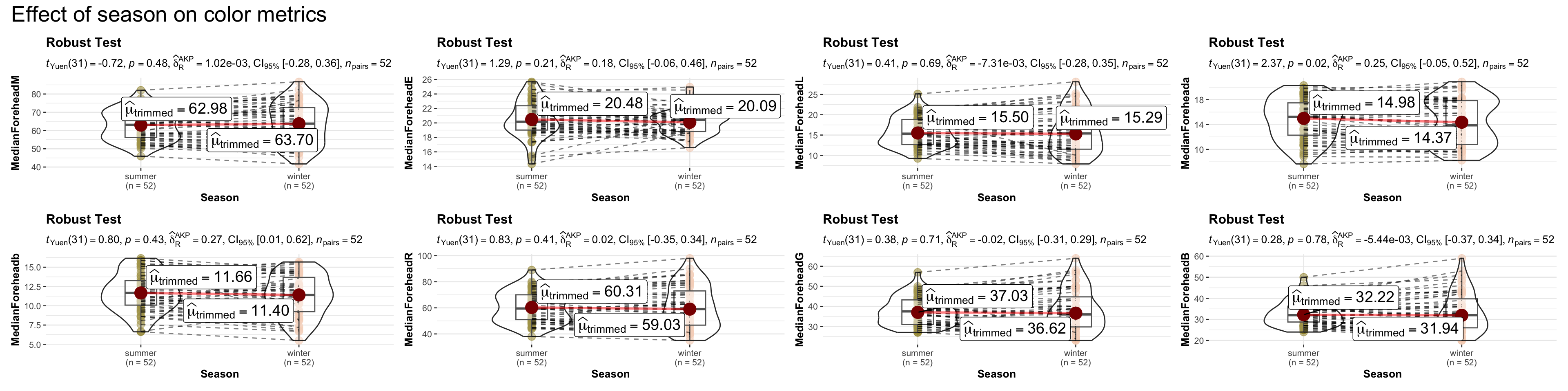
  annotation.args = list(
    title = "Effect of season on color metrics",
    theme = ggplot2::theme(
      plot.title = element_text(size = 20)
    )
  )
)

Past versions of unnamed-chunk-5-1.png

Version	Author	Date
d9fb6da	Lily Heald	2025-02-04

grouped_ggwithinstats(
  ## arguments relevant for ggwithinstats
  data = long_data,
  x = Season,
  y = MedianForeheadM,
  grouping.var = Ethnicity,
  xlab = "Season",
  ylab = "MedianForeheadM",
  type = "robust", ## type of test
  pairwise.display = "all", ## display only all pairwise comparisons
  p.adjust.method = "BH", ## adjust p-values for multiple tests using this method
  # ggtheme = ggthemes::theme_tufte(),
  package = "ggsci",
  palette = "default_jco",
  digits = 3,
  centrality.label.args = list(size  = 10),
  ## arguments relevant for combine_plots
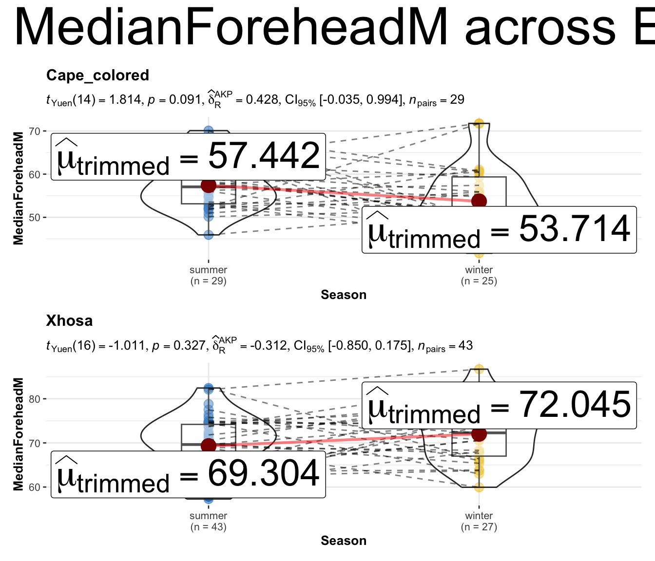
  annotation.args = list(title = "MedianForeheadM across Ethnicity",
                         theme = ggplot2::theme(plot.title = element_text(size = 40))),
  plotgrid.args = list(ncol = 1)
)

Past versions of unnamed-chunk-6-1.png

Version	Author	Date
d9fb6da	Lily Heald	2025-02-04

c1 <- grouped_ggwithinstats(
  ## arguments relevant for ggwithinstats
  data = long_data,
  x = Season,
  y = MedianForeheadL,
  grouping.var = Ethnicity,
  xlab = "Season",
  ylab = "MedianForeheadL",
  type = "nonparametric", ## type of test
  pairwise.display = "all", ## display only all pairwise comparisons
  p.adjust.method = "BH", ## adjust p-values for multiple tests using this method
  # ggtheme = ggthemes::theme_tufte(),
  package = "ggsci",
  palette = "default_jco",
  digits = 3,
  ## arguments relevant for combine_plots
  annotation.args = list(title = "MedianForeheadL across Ethnicity"),
  plotgrid.args = list(ncol = 1),
  ggplot.component = list(theme(text = element_text(size = 15)))
)

c2 <- grouped_ggwithinstats(
  ## arguments relevant for ggwithinstats
  data = long_data,
  x = Season,
  y = MedianForeheada,
  grouping.var = Ethnicity,
  xlab = "Season",
  ylab = "MedianForeheada",
  type = "nonparametric", ## type of test
  pairwise.display = "all", ## display only all pairwise comparisons
  p.adjust.method = "BH", ## adjust p-values for multiple tests using this method
  # ggtheme = ggthemes::theme_tufte(),
  package = "ggsci",
  palette = "default_jco",
  digits = 3,
  ## arguments relevant for combine_plots
  annotation.args = list(title = "MedianForeheada across Ethnicity"),
  plotgrid.args = list(ncol = 1),
  ggplot.component = list(theme(text = element_text(size = 15)))
)

c3 <- grouped_ggwithinstats(
  ## arguments relevant for ggwithinstats
  data = long_data,
  x = Season,
  y = MedianForeheadb,
  grouping.var = Ethnicity,
  xlab = "Season",
  ylab = "MedianForeheadb",
  type = "nonparametric", ## type of test
  pairwise.display = "all", ## display only all pairwise comparisons
  p.adjust.method = "BH", ## adjust p-values for multiple tests using this method
  # ggtheme = ggthemes::theme_tufte(),
  package = "ggsci",
  palette = "default_jco",
  digits = 3,
  ## arguments relevant for combine_plots
  annotation.args = list(title = "MedianForeheadb across Ethnicity"),
  plotgrid.args = list(ncol = 1),
  ggplot.component = list(theme(text = element_text(size = 15)))
)

c4 <- grouped_ggwithinstats(
  ## arguments relevant for ggwithinstats
  data = long_data,
  x = Season,
  y = InnerArmL,
  grouping.var = Ethnicity,
  xlab = "Season",
  ylab = "InnerArmL",
  type = "nonparametric", ## type of test
  pairwise.display = "all", ## display only all pairwise comparisons
  p.adjust.method = "BH", ## adjust p-values for multiple tests using this method
  # ggtheme = ggthemes::theme_tufte(),
  package = "ggsci",
  palette = "default_jco",
  digits = 3,
  ## arguments relevant for combine_plots
  annotation.args = list(title = "InnerArmL across Ethnicity"),
  plotgrid.args = list(ncol = 1),
  ggplot.component = list(theme(text = element_text(size = 15)))
)

c5 <- grouped_ggwithinstats(
  ## arguments relevant for ggwithinstats
  data = long_data,
  x = Season,
  y = InnerArma,
  grouping.var = Ethnicity,
  xlab = "Season",
  ylab = "InnerArma",
  type = "nonparametric", ## type of test
  pairwise.display = "all", ## display only all pairwise comparisons
  p.adjust.method = "BH", ## adjust p-values for multiple tests using this method
  # ggtheme = ggthemes::theme_tufte(),
  package = "ggsci",
  palette = "default_jco",
  digits = 3,
  ## arguments relevant for combine_plots
  annotation.args = list(title = "InnerArma across Ethnicity"),
  plotgrid.args = list(ncol = 1),
  ggplot.component = list(theme(text = element_text(size = 15)))
)

c6 <- grouped_ggwithinstats(
  ## arguments relevant for ggwithinstats
  data = long_data,
  x = Season,
  y = InnerArmb,
  grouping.var = Ethnicity,
  xlab = "Season",
  ylab = "InnerArmb",
  type = "nonparametric", ## type of test
  pairwise.display = "all", ## display only all pairwise comparisons
  p.adjust.method = "BH", ## adjust p-values for multiple tests using this method
  # ggtheme = ggthemes::theme_tufte(),
  package = "ggsci",
  palette = "default_jco",
  digits = 3,
  ## arguments relevant for combine_plots
  annotation.args = list(title = "InnerArmb across Ethnicity"),
  plotgrid.args = list(ncol = 1),
  ggplot.component = list(theme(text = element_text(size = 15)))
)

combine_plots(
  plotlist = list(c1, c2, c3, c4, c5, c6),
  plotgrid.args = list(nrow = 2),
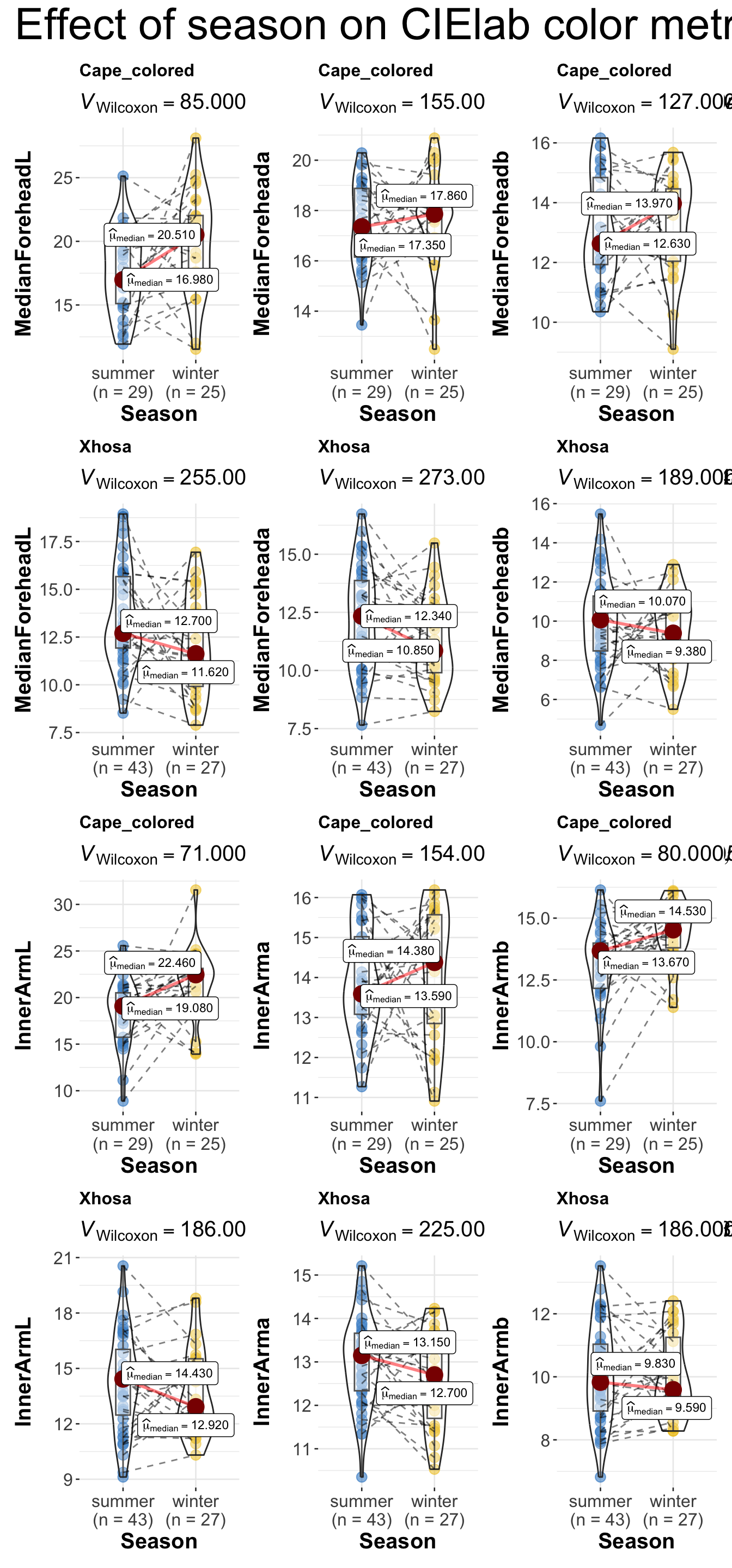
  annotation.args = list(
    title = "Effect of season on CIElab color metrics across ethnicity", 
    theme = ggplot2::theme(plot.title = element_text(size = 30)))
)

Past versions of unnamed-chunk-7-1.png

Version	Author	Date
d9fb6da	Lily Heald	2025-02-04

r1 <- grouped_ggwithinstats(
  ## arguments relevant for ggwithinstats
  data = long_data,
  x = Season,
  y = MedianForeheadR,
  grouping.var = Ethnicity,
  xlab = "Season",
  ylab = "MedianForeheadR",
  type = "nonparametric", ## type of test
  pairwise.display = "all", ## display only all pairwise comparisons
  p.adjust.method = "BH", ## adjust p-values for multiple tests using this method
  # ggtheme = ggthemes::theme_tufte(),
  package = "ggsci",
  palette = "default_jco",
  digits = 3,
  ## arguments relevant for combine_plots
  annotation.args = list(title = "MedianForeheadR across Ethnicity"),
  plotgrid.args = list(ncol = 1),
  ggplot.component = list(theme(text = element_text(size = 15)))
)

r2 <- grouped_ggwithinstats(
  ## arguments relevant for ggwithinstats
  data = long_data,
  x = Season,
  y = MedianForeheadG,
  grouping.var = Ethnicity,
  xlab = "Season",
  ylab = "MedianForeheadG",
  type = "nonparametric", ## type of test
  pairwise.display = "all", ## display only all pairwise comparisons
  p.adjust.method = "BH", ## adjust p-values for multiple tests using this method
  # ggtheme = ggthemes::theme_tufte(),
  package = "ggsci",
  palette = "default_jco",
  digits = 3,
  ## arguments relevant for combine_plots
  annotation.args = list(title = "MedianForeheadG across Ethnicity"),
  plotgrid.args = list(ncol = 1),
  ggplot.component = list(theme(text = element_text(size = 15)))
)

r3 <- grouped_ggwithinstats(
  ## arguments relevant for ggwithinstats
  data = long_data,
  x = Season,
  y = MedianForeheadB,
  grouping.var = Ethnicity,
  xlab = "Season",
  ylab = "MedianForeheadB",
  type = "nonparametric", ## type of test
  pairwise.display = "all", ## display only all pairwise comparisons
  p.adjust.method = "BH", ## adjust p-values for multiple tests using this method
  # ggtheme = ggthemes::theme_tufte(),
  package = "ggsci",
  palette = "default_jco",
  digits = 3,
  ## arguments relevant for combine_plots
  annotation.args = list(title = "MedianForeheadB across Ethnicity"),
  plotgrid.args = list(ncol = 1),
  ggplot.component = list(theme(text = element_text(size = 15)))
)

r4 <- grouped_ggwithinstats(
  ## arguments relevant for ggwithinstats
  data = long_data,
  x = Season,
  y = InnerArmR,
  grouping.var = Ethnicity,
  xlab = "Season",
  ylab = "InnerArmR",
  type = "nonparametric", ## type of test
  pairwise.display = "all", ## display only all pairwise comparisons
  p.adjust.method = "BH", ## adjust p-values for multiple tests using this method
  # ggtheme = ggthemes::theme_tufte(),
  package = "ggsci",
  palette = "default_jco",
  digits = 3,
  ## arguments relevant for combine_plots
  annotation.args = list(title = "InnerArmR across Ethnicity"),
  plotgrid.args = list(ncol = 1),
  ggplot.component = list(theme(text = element_text(size = 15)))
)

r5 <- grouped_ggwithinstats(
  ## arguments relevant for ggwithinstats
  data = long_data,
  x = Season,
  y = InnerArmG,
  grouping.var = Ethnicity,
  xlab = "Season",
  ylab = "InnerArmG",
  type = "nonparametric", ## type of test
  pairwise.display = "all", ## display only all pairwise comparisons
  p.adjust.method = "BH", ## adjust p-values for multiple tests using this method
  # ggtheme = ggthemes::theme_tufte(),
  package = "ggsci",
  palette = "default_jco",
  digits = 3,
  ## arguments relevant for combine_plots
  annotation.args = list(title = "InnerArmG across Ethnicity"),
  plotgrid.args = list(ncol = 1),
  ggplot.component = list(theme(text = element_text(size = 15)))
)

r6 <- grouped_ggwithinstats(
  ## arguments relevant for ggwithinstats
  data = long_data,
  x = Season,
  y = InnerArmB,
  grouping.var = Ethnicity,
  xlab = "Season",
  ylab = "InnerArmB",
  type = "nonparametric", ## type of test
  pairwise.display = "all", ## display only all pairwise comparisons
  p.adjust.method = "BH", ## adjust p-values for multiple tests using this method
  # ggtheme = ggthemes::theme_tufte(),
  package = "ggsci",
  palette = "default_jco",
  digits = 3,
  ## arguments relevant for combine_plots
  annotation.args = list(title = "InnerArmB across Ethnicity"),
  plotgrid.args = list(ncol = 1),
  ggplot.component = list(theme(text = element_text(size = 15)))
)

combine_plots(
  plotlist = list(r1, r2, r3, r4, r5, r6),
  plotgrid.args = list(nrow = 2),
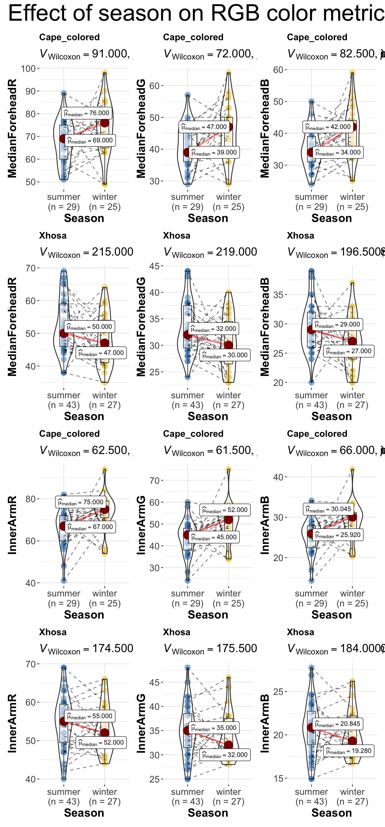
  annotation.args = list(
    title = "Effect of season on RGB color metrics across ethnicity", 
    theme = ggplot2::theme(plot.title = element_text(size = 30)))
)

Past versions of unnamed-chunk-8-1.png

Version	Author	Date
d9fb6da	Lily Heald	2025-02-04

m1 <- grouped_ggwithinstats(
  ## arguments relevant for ggwithinstats
  data = long_data,
  x = Season,
  y = MedianForeheadE,
  grouping.var = Ethnicity,
  xlab = "Season",
  ylab = "MedianForeheadE",
  type = "nonparametric", ## type of test
  pairwise.display = "all", ## display only all pairwise comparisons
  p.adjust.method = "BH", ## adjust p-values for multiple tests using this method
  # ggtheme = ggthemes::theme_tufte(),
  package = "ggsci",
  palette = "default_jco",
  digits = 3,
  ## arguments relevant for combine_plots
  annotation.args = list(title = "MedianForeheadE across Ethnicity"),
  plotgrid.args = list(ncol = 1)
)

m3 <- grouped_ggwithinstats(
  ## arguments relevant for ggwithinstats
  data = long_data,
  x = Season,
  y = InnerArmE,
  grouping.var = Ethnicity,
  xlab = "Season",
  ylab = "InnerArmE",
  type = "nonparametric", ## type of test
  pairwise.display = "all", ## display only all pairwise comparisons
  p.adjust.method = "BH", ## adjust p-values for multiple tests using this method
  # ggtheme = ggthemes::theme_tufte(),
  package = "ggsci",
  palette = "default_jco",
  digits = 3,
  ## arguments relevant for combine_plots
  annotation.args = list(title = "InnerArmE across Ethnicity"),
  plotgrid.args = list(ncol = 1)
)

m2 <- grouped_ggwithinstats(
  ## arguments relevant for ggwithinstats
  data = long_data,
  x = Season,
  y = MedianForeheadM,
  grouping.var = Ethnicity,
  xlab = "Season",
  ylab = "MedianForheadM",
  type = "nonparametric", ## type of test
  pairwise.display = "all", ## display only all pairwise comparisons
  p.adjust.method = "BH", ## adjust p-values for multiple tests using this method
  # ggtheme = ggthemes::theme_tufte(),
  package = "ggsci",
  palette = "default_jco",
  digits = 3,
  ## arguments relevant for combine_plots
  annotation.args = list(title = "MedianForheadM across Ethnicity"),
  plotgrid.args = list(ncol = 1)
)

m4 <- grouped_ggwithinstats(
  ## arguments relevant for ggwithinstats
  data = long_data,
  x = Season,
  y = InnerArmM,
  grouping.var = Ethnicity,
  xlab = "Season",
  ylab = "InnerArmM",
  type = "nonparametric", ## type of test
  pairwise.display = "all", ## display only all pairwise comparisons
  p.adjust.method = "BH", ## adjust p-values for multiple tests using this method
  # ggtheme = ggthemes::theme_tufte(),
  package = "ggsci",
  palette = "default_jco",
  digits = 3,
  ## arguments relevant for combine_plots
  annotation.args = list(title = "InnerArmM across Ethnicity"),
  plotgrid.args = list(ncol = 1)
)

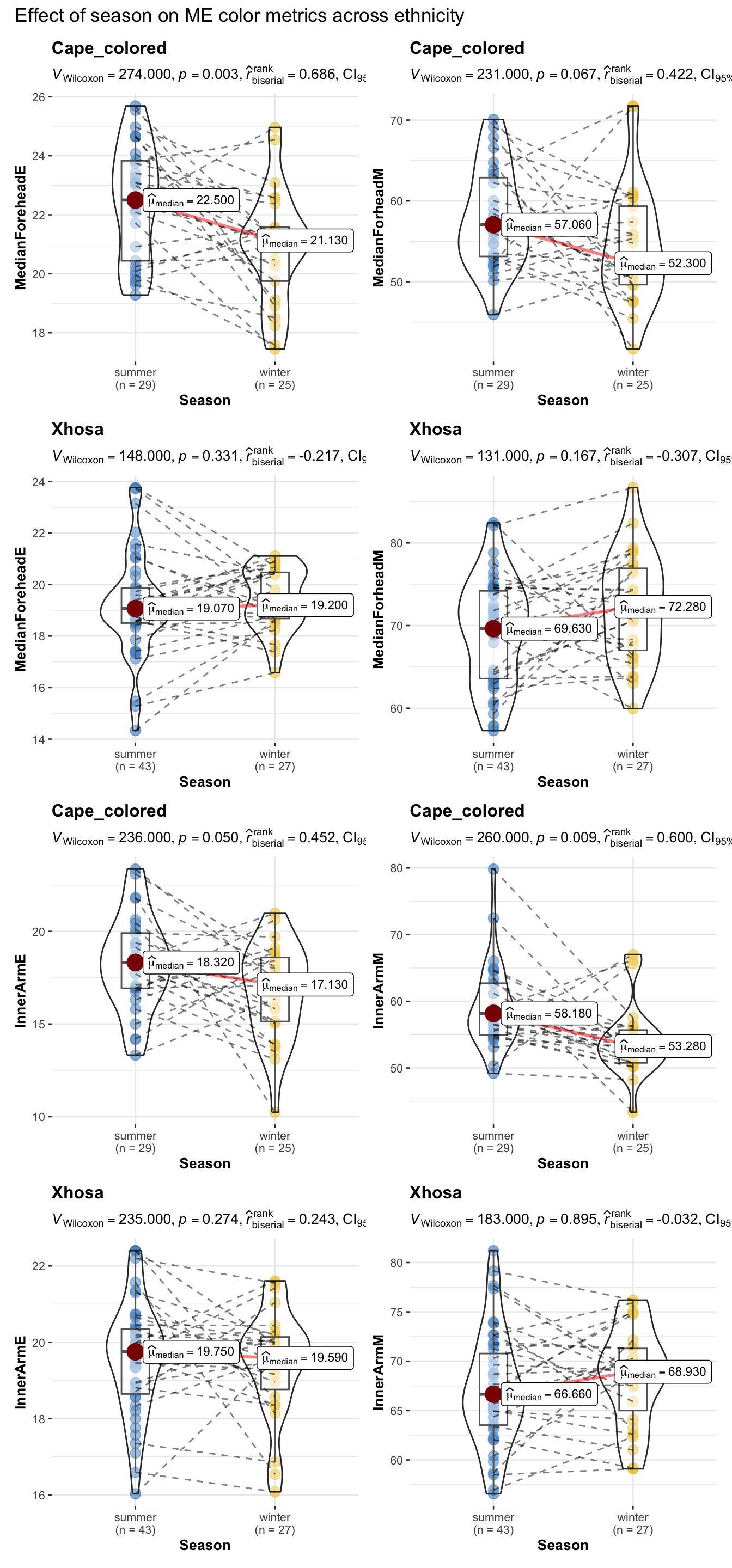
combine_plots(
  plotlist = list(m1, m2, m3, m4),
  plotgrid.args = list(nrow = 2),
  annotation.args = list(
    title = "Effect of season on ME color metrics across ethnicity")
)

Past versions of unnamed-chunk-9-1.png

Version	Author	Date
d9fb6da	Lily Heald	2025-02-04

p1 <- ggwithinstats(
  data = long_data,
  x = Season,
  y = MedianForeheadM,
  type = "p",
  effsize.type = "d",
  conf.level = 0.99,
  title = "Parametric test",
  package = "ggsci",
  palette = "nrc_npg"
)

## Mann-Whitney U test (nonparametric test)
p2 <- ggwithinstats(
  data = long_data,
  x = Season,
  y = MedianForeheadM,
  xlab = "Season",
  ylab = "MedianForeheadM
  ",
  type = "np",
  conf.level = 0.99,
  title = "Non-parametric Test",
  package = "ggsci",
  palette = "uniform_startrek"
)

## robust t-test
p3 <- ggwithinstats(
  data = long_data,
  x = Season,
  y = MedianForeheadM,
  xlab = "Season",
  ylab = "MedianForeheadM",
  type = "r",
  conf.level = 0.99,
  title = "Robust Test",
  package = "wesanderson",
  palette = "Royal2"
)

## Bayes Factor for parametric t-test
p4 <- ggwithinstats(
  data = long_data,
  x = Season,
  y = MedianForeheadM,
  xlab = "Season",
  ylab = "MedianForeheadM",
  type = "bayes",
  title = "Bayesian Test",
  package = "ggsci",
  palette = "nrc_npg"
)

# combining the individual plots into a single plot
combine_plots(
  plotlist = list(p1, p2, p3, p4),
  plotgrid.args = list(nrow = 2),
  annotation.args = list(
    title = "Effect of season on color metrics"),
  height = 10,  # Increase the height (adjust as needed)
  width = 12 
)

Past versions of unnamed-chunk-10-1.png

Version	Author	Date
d9fb6da	Lily Heald	2025-02-04

e1 <- ggwithinstats(
  data = summer_winter,
  x = Ethnicity_summer,
  y = MedianForeheadM_summer,
  xlab = "Ethnicity",
  ylab = "MedianForeheadM",
  type = "r",
  title = "Robust Test",
  package = "wesanderson",
  palette = "Royal2"
)

e2 <- ggwithinstats(
  data = summer_winter,
  x = Ethnicity_summer,
  y = MedianForeheadE_summer,
  xlab = "Ethnicity",
  ylab = "MedianForeheadE",
  type = "r",
  title = "Robust Test",
  package = "wesanderson",
  palette = "Royal2"
)

e3 <- ggwithinstats(
  data = summer_winter,
  x = Ethnicity_summer,
  y = MedianForeheadL_summer,
  xlab = "Ethnicity",
  ylab = "MedianForeheadL",
  type = "r",
  title = "Robust Test",
  package = "wesanderson",
  palette = "Royal2"
)

e4 <- ggwithinstats(
  data = summer_winter,
  x = Ethnicity_summer,
  y = MedianForeheada_summer,
  xlab = "Ethnicity",
  ylab = "MedianForeheada",
  type = "r",
  title = "Robust Test",
  package = "wesanderson",
  palette = "Royal2"
)

e5 <- ggwithinstats(
  data = summer_winter,
  x = Ethnicity_summer,
  y = MedianForeheadb_summer,
  xlab = "Ethnicity",
  ylab = "MedianForeheadb",
  type = "r",
  title = "Robust Test",
  package = "wesanderson",
  palette = "Royal2"
)

e6 <- ggwithinstats(
  data = summer_winter,
  x = Ethnicity_summer,
  y = MedianForeheadR_summer,
  xlab = "Ethnicity",
  ylab = "MedianForeheadR",
  type = "r",
  title = "Robust Test",
  package = "wesanderson",
  palette = "Royal2"
)

e7 <- ggwithinstats(
  data = summer_winter,
  x = Ethnicity_summer,
  y = MedianForeheadG_summer,
  xlab = "Ethnicity",
  ylab = "MedianForeheadG",
  type = "r",
  title = "Robust Test",
  package = "wesanderson",
  palette = "Royal2"
)

e8 <- ggwithinstats(
  data = summer_winter,
  x = Ethnicity_summer,
  y = MedianForeheadB_summer,
  xlab = "Ethnicity",
  ylab = "MedianForeheadB",
  type = "r",
  title = "Robust Test",
  package = "wesanderson",
  palette = "Royal2"
)

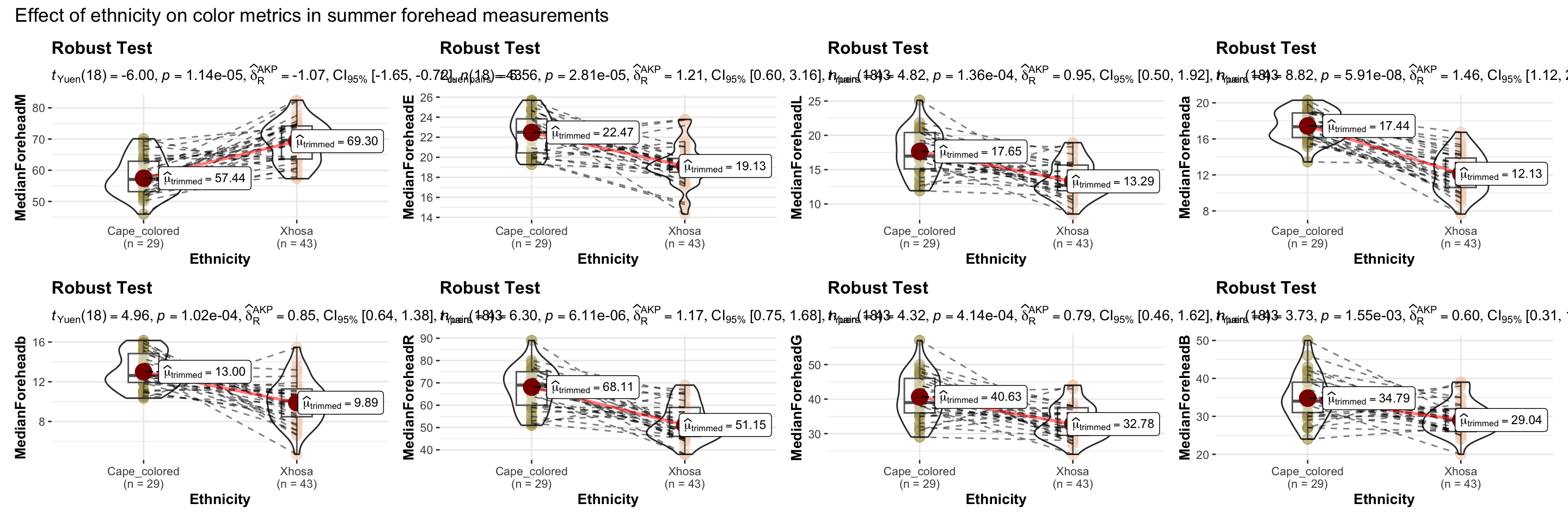
# combining the individual plots into a single plot
combine_plots(
  plotlist = list(e1, e2, e3, e4, e5, e6, e7, e8),
  plotgrid.args = list(nrow = 2),
  annotation.args = list(
    title = "Effect of ethnicity on color metrics in summer forehead measurements"),
  height = 10,  # Increase the height (adjust as needed)
  width = 12 
)

Past versions of unnamed-chunk-11-1.png

Version	Author	Date
d9fb6da	Lily Heald	2025-02-04

e1 <- ggwithinstats(
  data = summer_winter,
  x = Ethnicity_winter,
  y = MedianForeheadM_winter,
  xlab = "Ethnicity",
  ylab = "MedianForeheadM",
  type = "r",
  title = "Robust Test",
  package = "wesanderson",
  palette = "Royal2"
)

e2 <- ggwithinstats(
  data = summer_winter,
  x = Ethnicity_winter,
  y = MedianForeheadE_winter,
  xlab = "Ethnicity",
  ylab = "MedianForeheadE",
  type = "r",
  title = "Robust Test",
  package = "wesanderson",
  palette = "Royal2"
)

e3 <- ggwithinstats(
  data = summer_winter,
  x = Ethnicity_winter,
  y = MedianForeheadL_winter,
  xlab = "Ethnicity",
  ylab = "MedianForeheadL",
  type = "r",
  title = "Robust Test",
  package = "wesanderson",
  palette = "Royal2"
)

e4 <- ggwithinstats(
  data = summer_winter,
  x = Ethnicity_winter,
  y = MedianForeheada_winter,
  xlab = "Ethnicity",
  ylab = "MedianForeheada",
  type = "r",
  title = "Robust Test",
  package = "wesanderson",
  palette = "Royal2"
)

e5 <- ggwithinstats(
  data = summer_winter,
  x = Ethnicity_winter,
  y = MedianForeheadb_winter,
  xlab = "Ethnicity",
  ylab = "MedianForeheadb",
  type = "r",
  title = "Robust Test",
  package = "wesanderson",
  palette = "Royal2"
)

e6 <- ggwithinstats(
  data = summer_winter,
  x = Ethnicity_winter,
  y = MedianForeheadR_winter,
  xlab = "Ethnicity",
  ylab = "MedianForeheadR",
  type = "r",
  title = "Robust Test",
  package = "wesanderson",
  palette = "Royal2"
)

e7 <- ggwithinstats(
  data = summer_winter,
  x = Ethnicity_winter,
  y = MedianForeheadG_winter,
  xlab = "Ethnicity",
  ylab = "MedianForeheadG",
  type = "r",
  title = "Robust Test",
  package = "wesanderson",
  palette = "Royal2"
)

e8 <- ggwithinstats(
  data = summer_winter,
  x = Ethnicity_winter,
  y = MedianForeheadB_winter,
  xlab = "Ethnicity",
  ylab = "MedianForeheadB",
  type = "r",
  title = "Robust Test",
  package = "wesanderson",
  palette = "Royal2"
)

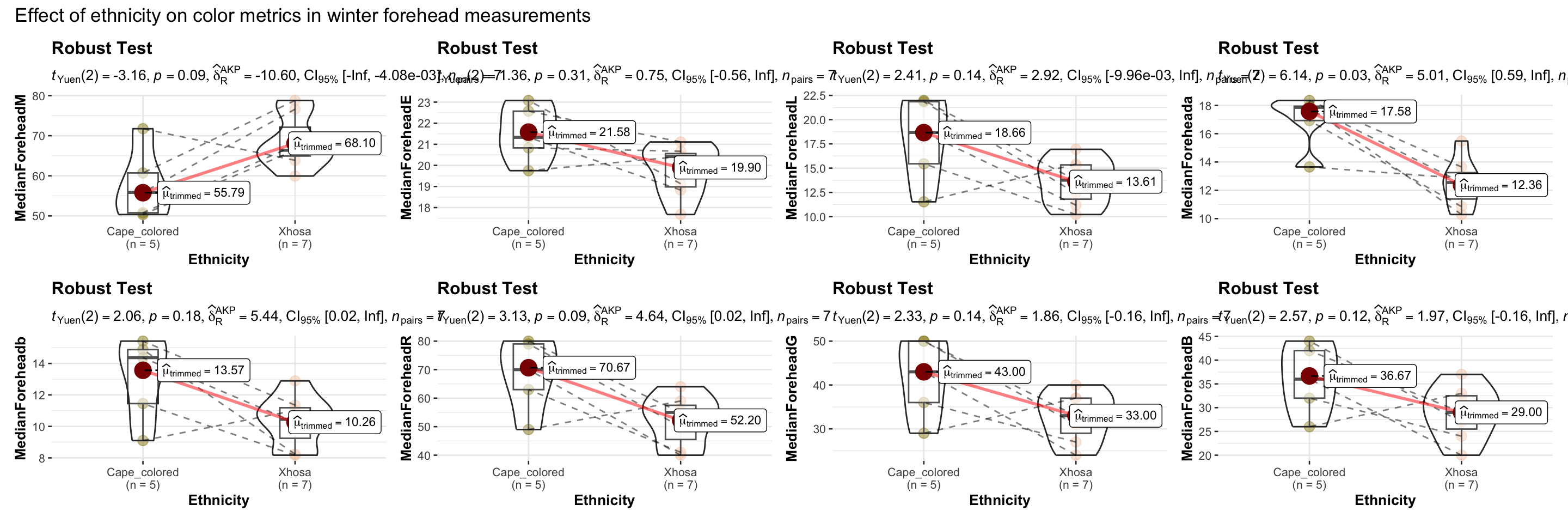
# combining the individual plots into a single plot
combine_plots(
  plotlist = list(e1, e2, e3, e4, e5, e6, e7, e8),
  plotgrid.args = list(nrow = 2),
  annotation.args = list(
    title = "Effect of ethnicity on color metrics in winter forehead measurements"),
  height = 10,  # Increase the height (adjust as needed)
  width = 12 
)

Past versions of unnamed-chunk-12-1.png

Version	Author	Date
d9fb6da	Lily Heald	2025-02-04

e1 <- ggwithinstats(
  data = summer_winter,
  x = Ethnicity_summer,
  y = InnerArmM_summer,
  xlab = "Ethnicity",
  ylab = "InnerArmM",
  type = "r",
  title = "Robust Test",
  package = "wesanderson",
  palette = "Royal2"
)

e2 <- ggwithinstats(
  data = summer_winter,
  x = Ethnicity_summer,
  y = InnerArmE_summer,
  xlab = "Ethnicity",
  ylab = "InnerArmE",
  type = "r",
  title = "Robust Test",
  package = "wesanderson",
  palette = "Royal2"
)

e3 <- ggwithinstats(
  data = summer_winter,
  x = Ethnicity_summer,
  y = InnerArmL_summer,
  xlab = "Ethnicity",
  ylab = "InnerArmL",
  type = "r",
  title = "Robust Test",
  package = "wesanderson",
  palette = "Royal2"
)

e4 <- ggwithinstats(
  data = summer_winter,
  x = Ethnicity_summer,
  y = InnerArma_summer,
  xlab = "Ethnicity",
  ylab = "InnerArma",
  type = "r",
  title = "Robust Test",
  package = "wesanderson",
  palette = "Royal2"
)

e5 <- ggwithinstats(
  data = summer_winter,
  x = Ethnicity_summer,
  y = InnerArmb_summer,
  xlab = "Ethnicity",
  ylab = "InnerArmb",
  type = "r",
  title = "Robust Test",
  package = "wesanderson",
  palette = "Royal2"
)

e6 <- ggwithinstats(
  data = summer_winter,
  x = Ethnicity_summer,
  y = InnerArmR_summer,
  xlab = "Ethnicity",
  ylab = "InnerArmR",
  type = "r",
  title = "Robust Test",
  package = "wesanderson",
  palette = "Royal2"
)

e7 <- ggwithinstats(
  data = summer_winter,
  x = Ethnicity_summer,
  y = InnerArmG_summer,
  xlab = "Ethnicity",
  ylab = "InnerArmG",
  type = "r",
  title = "Robust Test",
  package = "wesanderson",
  palette = "Royal2"
)

e8 <- ggwithinstats(
  data = summer_winter,
  x = Ethnicity_summer,
  y = InnerArmB_summer,
  xlab = "Ethnicity",
  ylab = "InnerArmB",
  type = "r",
  title = "Robust Test",
  package = "wesanderson",
  palette = "Royal2"
)

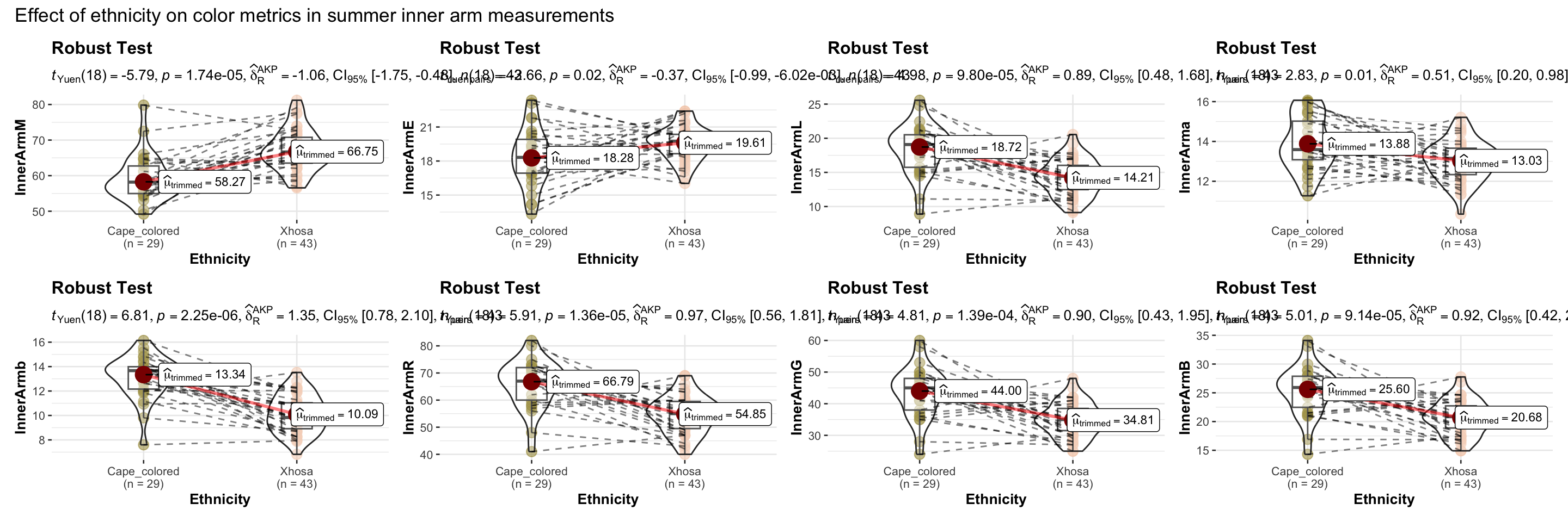
# combining the individual plots into a single plot
combine_plots(
  plotlist = list(e1, e2, e3, e4, e5, e6, e7, e8),
  plotgrid.args = list(nrow = 2),
  annotation.args = list(
    title = "Effect of ethnicity on color metrics in summer inner arm measurements"),
  height = 10,  # Increase the height (adjust as needed)
  width = 12 
)

Past versions of unnamed-chunk-13-1.png

Version	Author	Date
d9fb6da	Lily Heald	2025-02-04

e1 <- ggwithinstats(
  data = summer_winter,
  x = Ethnicity_winter,
  y = InnerArmM_winter,
  xlab = "Ethnicity",
  ylab = "InnerArmM",
  type = "r",
  title = "Robust Test",
  package = "wesanderson",
  palette = "Royal2"
)

e2 <- ggwithinstats(
  data = summer_winter,
  x = Ethnicity_winter,
  y = InnerArmE_winter,
  xlab = "Ethnicity",
  ylab = "InnerArmE",
  type = "r",
  title = "Robust Test",
  package = "wesanderson",
  palette = "Royal2"
)

e3 <- ggwithinstats(
  data = summer_winter,
  x = Ethnicity_winter,
  y = InnerArmL_winter,
  xlab = "Ethnicity",
  ylab = "InnerArmL",
  type = "r",
  title = "Robust Test",
  package = "wesanderson",
  palette = "Royal2"
)

e4 <- ggwithinstats(
  data = summer_winter,
  x = Ethnicity_winter,
  y = InnerArma_winter,
  xlab = "Ethnicity",
  ylab = "InnerArma",
  type = "r",
  title = "Robust Test",
  package = "wesanderson",
  palette = "Royal2"
)

e5 <- ggwithinstats(
  data = summer_winter,
  x = Ethnicity_winter,
  y = InnerArmb_winter,
  xlab = "Ethnicity",
  ylab = "InnerArmb",
  type = "r",
  title = "Robust Test",
  package = "wesanderson",
  palette = "Royal2"
)

e6 <- ggwithinstats(
  data = summer_winter,
  x = Ethnicity_winter,
  y = InnerArmR_winter,
  xlab = "Ethnicity",
  ylab = "InnerArmR",
  type = "r",
  title = "Robust Test",
  package = "wesanderson",
  palette = "Royal2"
)

e7 <- ggwithinstats(
  data = summer_winter,
  x = Ethnicity_winter,
  y = InnerArmG_winter,
  xlab = "Ethnicity",
  ylab = "InnerArmG",
  type = "r",
  title = "Robust Test",
  package = "wesanderson",
  palette = "Royal2"
)

e8 <- ggwithinstats(
  data = summer_winter,
  x = Ethnicity_winter,
  y = InnerArmB_winter,
  xlab = "Ethnicity",
  ylab = "InnerArmB",
  type = "r",
  title = "Robust Test",
  package = "wesanderson",
  palette = "Royal2"
)

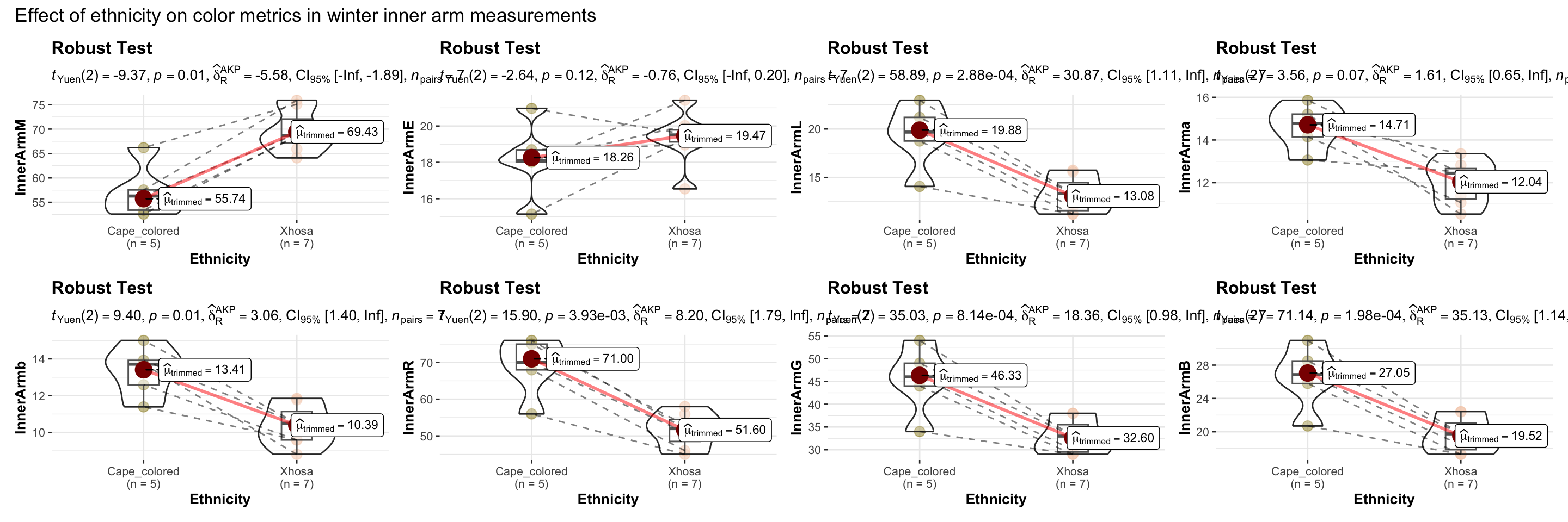
# combining the individual plots into a single plot
combine_plots(
  plotlist = list(e1, e2, e3, e4, e5, e6, e7, e8),
  plotgrid.args = list(nrow = 2),
  annotation.args = list(
    title = "Effect of ethnicity on color metrics in winter inner arm measurements"),
  height = 10,  # Increase the height (adjust as needed)
  width = 12 
)

Past versions of unnamed-chunk-14-1.png

Version	Author	Date
d9fb6da	Lily Heald	2025-02-04

linear mixed effects model

fixed effects: we expect will have an effect on the response variable

random effects: trying to control - season

Y_{ijk} = _0 + 1 + (1|) + {ijk}

messyjoin <- left_join(data_summer, data_winter, 
                     by = "ParticipantCentreID", 
                     suffix = c("_summer", "_winter"))
messyjoin <- messyjoin %>%
  select(matches("SkinReflectance|ParticipantCentreID|VitD"))
names(messyjoin) <- gsub("\\\\", "", names(messyjoin))
names(messyjoin) <- gsub("\\*", "", names(messyjoin))


df_long <- messyjoin %>%
  pivot_longer(
    cols = -ParticipantCentreID,  
    names_to = c("Site", "Metric", "Replicate", "Season"),
    names_pattern = "SkinReflectance(.*)([EMRGBLab])(\\d+)_(.*)",  
    values_to = "Value"
  )

df_long <- df_long %>%
  mutate(Ethnicity = case_when(
    grepl("^VDTG", ParticipantCentreID) ~ "CM",
    grepl("^VDKH", ParticipantCentreID) ~ "XH",
    TRUE ~ NA))

df_long$Season <- as.factor (df_long$Season) 
df_long$Ethnicity <- as.factor (df_long$Ethnicity)
head(df_long)

# A tibble: 6 × 7
  ParticipantCentreID Site     Metric Replicate Season Value Ethnicity
  <chr>               <chr>    <chr>  <chr>     <fct>  <dbl> <fct>    
1 VDKH001             Forehead E      1         summer  17.0 XH       
2 VDKH001             Forehead E      2         summer  18.7 XH       
3 VDKH001             Forehead E      3         summer  18.6 XH       
4 VDKH001             Forehead M      1         summer  56.0 XH       
5 VDKH001             Forehead M      2         summer  70.6 XH       
6 VDKH001             Forehead M      3         summer  76.3 XH       

melanin <- df_long[df_long$Metric == "M",]
erythema <- df_long[df_long$Metric == "E",]
library(lme4)

melanin.mixed.lmer <- lmer(Value ~ Ethnicity + Season + (1|ParticipantCentreID/Site) + (1|Replicate), data = melanin)

boundary (singular) fit: see help('isSingular')

melanin.reduced.lmer <- lmer(Value ~ 1 + (1|Season) + (1|ParticipantCentreID/Site) + (1|Replicate), data = melanin)

boundary (singular) fit: see help('isSingular')

a1 <- anova(melanin.reduced.lmer, melanin.mixed.lmer)

refitting model(s) with ML (instead of REML)

erythema.mixed.lmer <- lmer(Value ~ Ethnicity + Season + (1|ParticipantCentreID/Site) + (1|Replicate), data = erythema)

boundary (singular) fit: see help('isSingular')

erythema.reduced.lmer <- lmer(Value ~ 1 + (1|Season) + (1|ParticipantCentreID/Site) + (1|Replicate), data = erythema)

boundary (singular) fit: see help('isSingular')

a2 <- anova(erythema.reduced.lmer, erythema.mixed.lmer)

refitting model(s) with ML (instead of REML)

a1_new <- data.frame(a1)
a2_new <- data.frame(a2) 

anova_results <- data.frame(cbind(c("Ethnicity", "Residuals", "Ethnicity", "Residuals"), 
                                  rbind(a1_new, a2_new))) 
colnames(anova_results) <- c("","npar","AIC","BIC","logLik","deviance","Chisq","Df","Pr(>Chisq)" )
row.names(anova_results) <- NULL

library(kableExtra)

Attaching package: 'kableExtra'

The following object is masked from 'package:dplyr':

    group_rows

anova_results %>% kable("html", digits=2) %>% 
  kable_styling(bootstrap_options = "striped", full_width = F) %>% 
  pack_rows(., "Melanin", 1, 2) %>% # groups rows with label
  pack_rows(., "Erythema", 3, 4) # groups rows with label

	npar	AIC	BIC	logLik	deviance	Chisq	Df	Pr(>Chisq)
Melanin
Ethnicity	6	14911.18	14943.75	-7449.59	14899.18	NA	NA	NA
Residuals	7	14896.94	14934.94	-7441.47	14882.94	16.24	1	0
Erythema
Ethnicity	6	8148.99	8181.56	-4068.49	8136.99	NA	NA	NA
Residuals	7	8124.75	8162.74	-4055.37	8110.75	26.24	1	0

melanin1 <- stats::lm(formula = Value ~ Ethnicity + Season, data = melanin)
combine_plots(
  plotlist = list(
    ggcoefstats(melanin1) +
      ggplot2::labs(x = parse(text = "'regression coefficient' ~italic(beta)")),
    ggcoefstats(melanin.mixed.lmer) +
      ggplot2::labs(
        x = parse(text = "'regression coefficient' ~italic(beta)"),
        y = "fixed effects"
      )
  ),
  plotgrid.args = list(nrow = 2),
  annotation.args = list(title = "Relationship between MI value and ethnicity")
)

Random effect variances not available. Returned R2 does not account for random effects.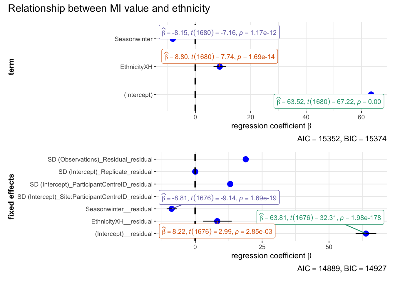

Past versions of effects-1.png

Version	Author	Date
d9fb6da	Lily Heald	2025-02-04

erythema1 <- stats::lm(formula = Value ~ Ethnicity + Season, data = erythema)
combine_plots(
  plotlist = list(
    ggcoefstats(erythema1) +
      ggplot2::labs(x = parse(text = "'regression coefficient' ~italic(beta)")),
    ggcoefstats(erythema.mixed.lmer) +
      ggplot2::labs(
        x = parse(text = "'regression coefficient' ~italic(beta)"),
        y = "fixed effects"
      )
  ),
  plotgrid.args = list(nrow = 2),
  annotation.args = list(title = "Relationship between EI value and ethnicity")
)

Random effect variances not available. Returned R2 does not account for random effects.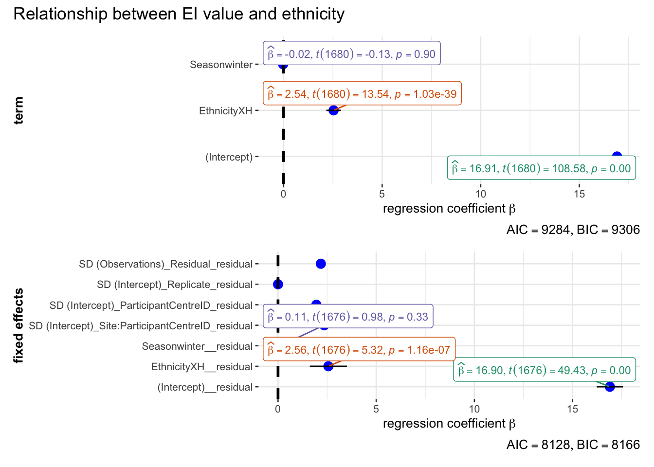

Past versions of effects-2.png

Version	Author	Date
d9fb6da	Lily Heald	2025-02-04

Session information

sessionInfo()

R version 4.4.2 (2024-10-31)
Platform: aarch64-apple-darwin20
Running under: macOS Monterey 12.5.1

Matrix products: default
BLAS:   /Library/Frameworks/R.framework/Versions/4.4-arm64/Resources/lib/libRblas.0.dylib 
LAPACK: /Library/Frameworks/R.framework/Versions/4.4-arm64/Resources/lib/libRlapack.dylib;  LAPACK version 3.12.0

locale:
[1] en_US.UTF-8/en_US.UTF-8/en_US.UTF-8/C/en_US.UTF-8/en_US.UTF-8

time zone: America/Detroit
tzcode source: internal

attached base packages:
[1] stats     graphics  grDevices utils     datasets  methods   base     

other attached packages:
 [1] kableExtra_1.4.0   ggstatsplot_0.13.0 lme4_1.1-36        Matrix_1.7-1      
 [5] rstatix_0.7.2      ggpubr_0.6.0       ggfortify_0.4.17   wesanderson_0.3.7 
 [9] missMDA_1.19       FactoMineR_2.11    factoextra_1.0.7   ggcorrplot_0.1.4.1
[13] corrr_0.4.4        readxl_1.4.3       lubridate_1.9.4    forcats_1.0.0     
[17] stringr_1.5.1      purrr_1.0.2        tibble_3.2.1       ggplot2_3.5.1     
[21] tidyverse_2.0.0    tidyr_1.3.1        dplyr_1.1.4        readr_2.1.5       
[25] workflowr_1.7.1   

loaded via a namespace (and not attached):
  [1] rstudioapi_0.17.1      jsonlite_1.8.9         shape_1.4.6.1         
  [4] correlation_0.8.6      datawizard_1.0.0       magrittr_2.0.3        
  [7] TH.data_1.1-3          estimability_1.5.1     jomo_2.7-6            
 [10] farver_2.1.2           nloptr_2.1.1           rmarkdown_2.29        
 [13] fs_1.6.5               vctrs_0.6.5            minqa_1.2.8           
 [16] paletteer_1.6.0        effectsize_1.0.0       htmltools_0.5.8.1     
 [19] broom_1.0.7            cellranger_1.1.0       Formula_1.2-5         
 [22] mitml_0.4-5            sass_0.4.9             bslib_0.8.0           
 [25] htmlwidgets_1.6.4      plyr_1.8.9             sandwich_3.1-1        
 [28] emmeans_1.10.6         zoo_1.8-12             cachem_1.1.0          
 [31] whisker_0.4.1          lifecycle_1.0.4        iterators_1.0.14      
 [34] pkgconfig_2.0.3        R6_2.5.1               fastmap_1.2.0         
 [37] rbibutils_2.3          BayesFactor_0.9.12-4.7 digest_0.6.37         
 [40] reshape_0.8.9          colorspace_2.1-1       rematch2_2.1.2        
 [43] patchwork_1.3.0        ps_1.8.1               rprojroot_2.0.4       
 [46] prismatic_1.1.2        labeling_0.4.3         WRS2_1.1-6            
 [49] timechange_0.3.0       httr_1.4.7             abind_1.4-8           
 [52] compiler_4.4.2         withr_3.0.2            doParallel_1.0.17     
 [55] backports_1.5.0        carData_3.0-5          performance_0.13.0    
 [58] ggsignif_0.6.4         pan_1.9                MASS_7.3-64           
 [61] scatterplot3d_0.3-44   flashClust_1.01-2      tools_4.4.2           
 [64] httpuv_1.6.15          statsExpressions_1.6.2 nnet_7.3-20           
 [67] glue_1.8.0             callr_3.7.6            nlme_3.1-166          
 [70] promises_1.3.2         grid_4.4.2             getPass_0.2-4         
 [73] cluster_2.1.8          generics_0.1.3         gtable_0.3.6          
 [76] tzdb_0.4.0             hms_1.1.3              xml2_1.3.6            
 [79] utf8_1.2.4             car_3.1-3              ggrepel_0.9.6         
 [82] foreach_1.5.2          pillar_1.10.1          later_1.4.1           
 [85] splines_4.4.2          lattice_0.22-6         survival_3.8-3        
 [88] tidyselect_1.2.1       pbapply_1.7-2          knitr_1.49            
 [91] git2r_0.35.0           reformulas_0.4.0       gridExtra_2.3         
 [94] svglite_2.1.3          xfun_0.50              DT_0.33               
 [97] stringi_1.8.4          yaml_2.3.10            boot_1.3-31           
[100] evaluate_1.0.3         codetools_0.2-20       multcompView_0.1-10   
[103] cli_3.6.3              RcppParallel_5.1.10    rpart_4.1.24          
[106] systemfonts_1.2.0      xtable_1.8-4           parameters_0.24.1     
[109] Rdpack_2.6.2           munsell_0.5.1          processx_3.8.5        
[112] jquerylib_0.1.4        Rcpp_1.0.14            zeallot_0.1.0         
[115] coda_0.19-4.1          parallel_4.4.2         MatrixModels_0.5-3    
[118] rstantools_2.4.0       leaps_3.2              bayestestR_0.15.0     
[121] glmnet_4.1-8           viridisLite_0.4.2      mvtnorm_1.3-3         
[124] scales_1.3.0           insight_1.0.1          rlang_1.1.4           
[127] multcomp_1.4-28        mice_3.17.0