Running the meta-analysis
Last updated: 2026-03-04
Checks: 7 0
Knit directory: exp_evol_metaanalysis/
This reproducible R Markdown analysis was created with workflowr (version 1.7.2). The Checks tab describes the reproducibility checks that were applied when the results were created. The Past versions tab lists the development history.
Great! Since the R Markdown file has been committed to the Git repository, you know the exact version of the code that produced these results.
Great job! The global environment was empty. Objects defined in the global environment can affect the analysis in your R Markdown file in unknown ways. For reproduciblity it’s best to always run the code in an empty environment.
The command set.seed(20260206) was run prior to running
the code in the R Markdown file. Setting a seed ensures that any results
that rely on randomness, e.g. subsampling or permutations, are
reproducible.
Great job! Recording the operating system, R version, and package versions is critical for reproducibility.
Nice! There were no cached chunks for this analysis, so you can be confident that you successfully produced the results during this run.
Great job! Using relative paths to the files within your workflowr project makes it easier to run your code on other machines.
Great! You are using Git for version control. Tracking code development and connecting the code version to the results is critical for reproducibility.
The results in this page were generated with repository version ba4bca1. See the Past versions tab to see a history of the changes made to the R Markdown and HTML files.
Note that you need to be careful to ensure that all relevant files for
the analysis have been committed to Git prior to generating the results
(you can use wflow_publish or
wflow_git_commit). workflowr only checks the R Markdown
file, but you know if there are other scripts or data files that it
depends on. Below is the status of the Git repository when the results
were generated:
Ignored files:
    Ignored:    .DS_Store
    Ignored:    .Rproj.user/
    Ignored:    input_data/.DS_Store
    Ignored:    input_data/lundhansen_github_data_FLXevoexp-master/.DS_Store
    Ignored:    input_data/lundhansen_github_data_FLXevoexp-master/DevelopmentTimeGeneration/.Rapp.history
    Ignored:    input_data/lundhansen_github_data_FLXevoexp-master/LocomotionAssayGeneration123/.DS_Store
    Ignored:    input_data/lundhansen_github_data_FLXevoexp-master/LocomotionAssayGeneration123/.Rapp.history
    Ignored:    input_data/lundhansen_github_data_FLXevoexp-master/LocomotionAssayGeneration123/.Rhistory
    Ignored:    input_data/lundhansen_github_data_FLXevoexp-master/ReproductiveFitnessFM/.Rapp.history
    Ignored:    input_data/lundhansen_github_data_FLXevoexp-master/ReproductiveFitnessFM/.Rhistory
    Ignored:    input_data/lundhansen_github_data_FLXevoexp-master/StandardFitnessGeneration15-18/.Rapp.history
    Ignored:    input_data/lundhansen_github_data_FLXevoexp-master/StandardFitnessGeneration39-41 /.Rapp.history
    Ignored:    input_data/lundhansen_github_data_FLXevoexp-master/ThoraxSizeGeneration15-18/.Rapp.history
    Ignored:    input_data/lundhansen_github_data_FLXevoexp-master/ThoraxSizeGeneration72/.Rapp.history

Untracked files:
    Untracked:  effect_sizes/MeloGavin2026.csv
    Untracked:  effect_sizes/jiang_2011_1.csv
    Untracked:  effect_sizes/jiang_2011_2.csv
    Untracked:  effect_sizes/jiang_2011_3.csv
    Untracked:  effect_sizes/jiang_2011_4.csv
    Untracked:  effect_sizes/prasad2007_1.csv
    Untracked:  effect_sizes/prasad2007_2.csv
    Untracked:  effect_sizes/prasad2007_3.csv
    Untracked:  effect_sizes/prasad2007_4.csv
    Untracked:  effect_sizes/prasad2007_5.csv
    Untracked:  effect_sizes/prasad2007_6.csv
    Untracked:  effect_sizes/thyagarajan2025_4.csv

Unstaged changes:
    Modified:   analysis/primary_data.Rmd
    Deleted:    data/README.md
    Modified:   effect_sizes/abbott2010_1.csv
    Modified:   effect_sizes/abbott2010_2.csv
    Modified:   effect_sizes/abbott2010_5.csv
    Modified:   effect_sizes/abbott2010_6.csv
    Modified:   effect_sizes/abbott_2013_1.csv
    Modified:   effect_sizes/abbott_2013_2.csv
    Modified:   effect_sizes/abbott_2020_2.csv
    Modified:   effect_sizes/bedhomme2008_1.csv
    Modified:   effect_sizes/manat_3.csv
    Modified:   effect_sizes/manat_4.csv
    Deleted:    effect_sizes/martinossiAllibert2019_1.csv
    Deleted:    effect_sizes/martinossiAllibert2019_2.csv
    Modified:   effect_sizes/melo_gavin2025_maleharm.csv
    Modified:   effect_sizes/norden2020.csv
    Modified:   effect_sizes/rice98_2.csv
    Modified:   effect_sizes/rice98_3.csv
    Modified:   effect_sizes/rice98_4.csv
    Modified:   effect_sizes/thyagarajan2025_2.csv
    Modified:   effect_sizes/thyagarajan2025_3.csv
    Modified:   input_data/study_metadata.csv
    Deleted:    output/README.md
Note that any generated files, e.g. HTML, png, CSS, etc., are not included in this status report because it is ok for generated content to have uncommitted changes.
These are the previous versions of the repository in which changes were
made to the R Markdown (analysis/meta_analysis.Rmd) and
HTML (docs/meta_analysis.html) files. If you’ve configured
a remote Git repository (see ?wflow_git_remote), click on
the hyperlinks in the table below to view the files as they were in that
past version.
| File | Version | Author | Date | Message |
|---|---|---|---|---|
| Rmd | ba4bca1 | luekholman | 2026-03-04 | wflow_publish("analysis/meta_analysis.Rmd") |
| html | ea73e7f | luekholman | 2026-03-03 | Build site. |
| Rmd | e8d6438 | luekholman | 2026-03-03 | wflow_publish("analysis/meta_analysis.Rmd") |
| html | 25b7e79 | luekholman | 2026-03-03 | Build site. |
| Rmd | 12d7808 | luekholman | 2026-03-03 | wflow_publish("analysis/meta_analysis.Rmd") |
| html | 8cb0ab7 | luekholman | 2026-03-03 | Build site. |
| Rmd | 2da5b5d | luekholman | 2026-03-03 | wflow_publish("analysis/meta_analysis.Rmd") |
| html | be1bcf7 | luekholman | 2026-03-03 | Build site. |
| Rmd | 0361b84 | luekholman | 2026-03-03 | wflow_publish("analysis/meta_analysis.Rmd") |
| html | 99fbc3e | luekholman | 2026-02-27 | Build site. |
| Rmd | 42e8e4c | luekholman | 2026-02-27 | wflow_publish("analysis/meta_analysis.Rmd") |
| html | a5fa098 | luekholman | 2026-02-27 | Build site. |
| Rmd | 0b19c38 | luekholman | 2026-02-27 | wflow_publish("analysis/meta_analysis.Rmd") |
| html | b10e003 | luekholman | 2026-02-27 | Build site. |
| Rmd | 9b3a028 | luekholman | 2026-02-27 | improved figure |
| html | 8915f97 | luekholman | 2026-02-27 | Build site. |
| Rmd | d6deab4 | luekholman | 2026-02-27 | improved figure |
| html | 65e7263 | luekholman | 2026-02-27 | Build site. |
| Rmd | ad9d4d5 | luekholman | 2026-02-27 | Improve figure |
| html | c6491af | luekholman | 2026-02-27 | Build site. |
| Rmd | e2a271b | luekholman | 2026-02-27 | Improve figure |
| html | c3874eb | luekholman | 2026-02-27 | Build site. |
| Rmd | 1bc8273 | luekholman | 2026-02-27 | Improve figure |
| html | 0b90819 | luekholman | 2026-02-27 | Build site. |
| Rmd | 0ffe753 | luekholman | 2026-02-27 | Improve figure |
| html | 4a05564 | luekholman | 2026-02-27 | Build site. |
| Rmd | ac24f2c | luekholman | 2026-02-27 | Improve figure |
| html | 1945697 | luekholman | 2026-02-26 | Build site. |
| Rmd | 6686ad2 | luekholman | 2026-02-26 | Figure improvements |
| html | 8d9eb2b | luekholman | 2026-02-26 | Build site. |
| Rmd | 734cb56 | luekholman | 2026-02-26 | Figure improvements |
| html | f80a6dd | luekholman | 2026-02-26 | Build site. |
| html | 0560e72 | luekholman | 2026-02-26 | Build site. |
| html | cbdc84d | luekholman | 2026-02-25 | Build site. |
| Rmd | 6aca63a | luekholman | 2026-02-25 | Edit Melo-Gavin 2025 and delete M-R |
| html | ff5afc8 | luekholman | 2026-02-20 | Build site. |
| Rmd | 9e651b1 | luekholman | 2026-02-20 | Add Melo-Gavin 2025 |
| html | 4719bf8 | luekholman | 2026-02-20 | Build site. |
| Rmd | b781d82 | luekholman | 2026-02-20 | Add Melo-Gavin 2025 |
| html | 3f80499 | luekholman | 2026-02-10 | Build site. |
| Rmd | 788847e | luekholman | 2026-02-10 | Fixed a few bits |
| html | f546a4c | luekholman | 2026-02-10 | Build site. |
| Rmd | 2e563e5 | luekholman | 2026-02-10 | Fixed a few bits |
| html | 68e88ca | luekholman | 2026-02-09 | Build site. |
| Rmd | 67d1c7a | luekholman | 2026-02-09 | pm typo |
| html | 67d1c7a | luekholman | 2026-02-09 | pm typo |
| html | 77d88f0 | luekholman | 2026-02-09 | Build site. |
| Rmd | d64f5ed | luekholman | 2026-02-09 | figure caption |
| html | 0b01f66 | luekholman | 2026-02-09 | Build site. |
| html | 27f0459 | luekholman | 2026-02-09 | Build site. |
| html | b0251e4 | luekholman | 2026-02-09 | Many minor edits |
| html | f4fb206 | luekholman | 2026-02-09 | First commit |
| html | f1a4d10 | luekholman | 2026-02-09 | First commit |
| html | 6029ddf | luekholman | 2026-02-09 | Build site. |
| Rmd | 7057ba1 | luekholman | 2026-02-09 | First commit |
| html | 7057ba1 | luekholman | 2026-02-09 | First commit |
Load packages, the meta-analysis data, and a helper function.
library(tidyverse)
library(metafor)
library(DT)
library(ggh4x)
library(kableExtra)


# function to make the searchable, exportable HTML table
my_data_table <- function(df){

  num_cols <- names(df)[sapply(df, is.numeric)]
  num_cols <- num_cols[num_cols != "Generations"]

  datatable(
    df, rownames = FALSE,
    autoHideNavigation = TRUE,
    extensions = c("Scroller", "Buttons"),
    options = list(
      autoWidth = TRUE,
      dom = 'Bfrtip',
      deferRender = TRUE,
      scrollX = TRUE,
      scrollY = 1000,
      scrollCollapse = TRUE,
      buttons = list(
        'pageLength',
        'colvis',
        list(
          extend = 'csv',
          filename = 'holman_meta_analysis'
        )
      ),
      pageLength = 100
    )
  ) %>%
    formatRound(
      columns = num_cols,
      digits = 3
    )
}

# Text formatters
pretty2 <- function(x) {
  formatC(x, format = "f", digits = 2)
}

pretty3 <- function(x) {
  formatC(x, format = "f", digits = 3)
}


# Load up the meta-analysis data:
meta_analysis_data <- list.files("effect_sizes/", full.names = T) %>%
  lapply(read_csv, show_col_types = FALSE) %>%
  bind_rows() %>%
  left_join(read_csv("input_data/study_metadata.csv"), by = join_by(Study)) %>%
  mutate(year = str_extract(Short_name, "[:digit:]+")) %>%
  arrange(year) %>%
  mutate(
    first_word = map_chr(str_split(Trait, " "), ~.x[[1]]),
    Sex = NA,
    Sex = replace(Sex, first_word %in% c("Male", "Sperm", "Mating"), "Male"),
    Sex = replace(Sex, first_word %in% c("Viability", "Egg-to-adult"), "Both"),
    Sex = replace(Sex, first_word == "Female", "Female")) %>%
  select(-first_word)
Data collected for the meta-analysis
This table is scrollable, searchable, and can be exported as a
.csv file. You can also sort by column, or hide columns.
The table lists 70 effect sizes (and their associated variance and 95%
CIs) from 11 independent experimental evolution projects, which were
published across 19 journal articles. The Trait column
gives the name of the trait being measured, Generations
gives the number of generations of selection before measuring this
trait, Interpretation gives a plain English description of
what the effect size means, Origin_of_lines column gives
the reference that first created the lines, the two
Experiment_type columns are two ways of categorising the
type of experiment, and Sex gives the sex of the
individuals being measured
meta_analysis_data %>%
  select(-year, -Short_name) %>%
  my_data_table()
Meta-analysis without moderators
This meta-analysis can be used to calculate the grand mean effect
size. It’s a mixed effects meta-analysis with the random effects
structure ~ 1 | Origin_of_lines/Study. This means we fit a
random intercept for Origin_of_lines, a variable which
gives the name of the study that first created the experimental
evolution lines being measured. We also fit a random intercept for
Study nested within Origin_of_lines, where
Study is a variable giving the name of the study doing the
measuring (which is often the same study, but not always, since some
studies re-measured lines that were created in an earlier study).
meta_analysis <- rma.mv(
  yi = Estimate,
  V = Var,
  random = ~ 1 | Origin_of_lines/Study,
  data = meta_analysis_data,
  method = "REML"
)

summary(meta_analysis)
Multivariate Meta-Analysis Model (k = 70; method: REML)

   logLik   Deviance        AIC        BIC       AICc
-471.2448   942.4895   948.4895   955.1919   948.8588

Variance Components:

            estim    sqrt  nlvls  fixed                 factor
sigma^2.1  0.0000  0.0000     11     no        Origin_of_lines
sigma^2.2  0.1257  0.3546     19     no  Origin_of_lines/Study

Test for Heterogeneity:
Q(df = 69) = 1351.2730, p-val < .0001

Model Results:

estimate      se    zval    pval   ci.lb   ci.ub
  0.3175  0.0847  3.7500  0.0002  0.1516  0.4835  ***

---
Signif. codes:  0 '***' 0.001 '**' 0.01 '*' 0.05 '.' 0.1 ' ' 1
The above results table shows that the grand mean effect size is 0.318, with a standard error of 0.085 and 95% CIs of 0.152 to 0.484.
Testing for effects of moderators
Here, I use AICc model selection to compare 7 competing meta-analysis
models, which fit Generations, Sex,
Experiment_type, a combination of 2 or all of these, or the
intercept-only null model. Generations gives the number of
generations of selection at the time the focal trait was measured,
Sex gives the sex of the individuals expressing the trait
(male, female, or both sexes), and Experiment_type is
either “Sex-specific autosome(s)”, “Sex-specific X”, or “Sex-specific
relaxed selection” (as described by the point colours in Figure 1).
The top model includes the moderator Generations, and it
is ahead of second-best model (which also includes Sex) by
more than 2 AICc, suggesting that Generations explains
substantial variation in the data but the other moderators do not.
fit_ma <- function(formula){

  # there are only 2 effect sizes relating to both sexes, so they crash the model. Just remove from this moderator analysis. Also scale the generations variable to mean 0, variance 1.
  scaled_meta_analysis_data <-
    meta_analysis_data %>%
    mutate(Generations = as.numeric(scale(Generations))) %>%
    filter(Sex != "Both")

  if(formula == "Intercept only"){
    return(meta_analysis)
  }

  rma.mv(
    yi = Estimate,
    V = Var,
    mods = as.formula(formula),
    random = ~ 1 | Origin_of_lines/Short_name,
    data = scaled_meta_analysis_data,
    method = "REML"
  )
}

fit_all <- function(formulae){
  meta <- lapply(formulae, fit_ma)
  get_p <- function(ma) as.numeric(ma$p)
  get_logLik <- function(ma) as.numeric(logLik(ma))
  get_AICc <- function(ma) as.numeric(AIC(ma, correct = T))

  data.frame(
    Model = formulae,
    k     = sapply(meta, get_p),
    logLik = sapply(meta, get_logLik),
    AICc   = sapply(meta, get_AICc)) %>%
    arrange(AICc) %>%
    mutate(Model = str_remove_all(Model, "~ "),
           delta_AICc = round(AICc - AICc[1], 2),
           delta_AICc = c(" ", delta_AICc[2:length(delta_AICc)]))
}

fit_all(c("~ Generations + Sex + Experiment_type1",
          "~ Generations + Sex",
          "~ Sex + Experiment_type1",
          "~ Generations",
          "~ Sex",
          "~ Experiment_type1",
          "Intercept only")) %>%
  kable() %>%
kable_styling(full_width = FALSE)| Model | k | logLik | AICc | delta_AICc |
|---|---|---|---|---|
| Generations | 2 | -463.7275 | 936.1107 | |
| Generations + Sex | 3 | -463.8714 | 938.7598 | 2.65 |
| Generations + Sex + Experiment_type1 | 5 | -462.2431 | 940.5225 | 4.41 |
| Intercept only | 1 | -471.2448 | 948.8588 | 12.75 |
| Experiment_type1 | 3 | -469.7447 | 950.5064 | 14.4 |
| Sex | 2 | -473.4629 | 955.5815 | 19.47 |
| Sex + Experiment_type1 | 4 | -471.7089 | 956.8915 | 20.78 |
Below are the results of the top model (ranked by AICc) with one or
more moderators, showing the significant negative effect of the
moderator Generations on effect size (note:
Generations was scaled to have mean 0, SD 1, prior to
analysis). This is a counter-intuitive result since we might expect
greater effects after more generations of selection, but it is not very
informative since Generations is confounded with other
factors (e.g. species, type of experimental design, type of trait being
measured, and whether I used the raw data or summary statistics to
calculate effect size). The grand mean effect size (predicted here for
the average value of Generations, which is 50.6) is 0.318
(0.168-0.468), which is much the same as the previous meta-analysis that
did not adjust for the effect of Generations.
fit_ma("~ Generations")
Multivariate Meta-Analysis Model (k = 68; method: REML)

Variance Components:

            estim    sqrt  nlvls  fixed                      factor
sigma^2.1  0.0000  0.0000     11     no             Origin_of_lines
sigma^2.2  0.1002  0.3166     19     no  Origin_of_lines/Short_name

Test for Residual Heterogeneity:
QE(df = 66) = 1316.8074, p-val < .0001

Test of Moderators (coefficient 2):
QM(df = 1) = 16.9666, p-val < .0001

Model Results:

             estimate      se     zval    pval    ci.lb    ci.ub
intrcpt        0.3180  0.0763   4.1657  <.0001   0.1684   0.4676  ***
Generations   -0.1181  0.0287  -4.1190  <.0001  -0.1743  -0.0619  ***

---
Signif. codes:  0 '***' 0.001 '**' 0.01 '*' 0.05 '.' 0.1 ' ' 1
Forest plot of effect sizes (Figure 1)
exp2_levs <- c("Male-limited haplotypes",
               "Male-limited autosome",
               "Female-limited markers",
               "Reciprocal sex-limited markers",
               "Symmetrical sex-limited autosomes",
               "Male-limited X chromosomes",
               "Female-limited X chromosomes",
               "Relaxed selection in females",
               "Relaxed selection in both sexes")

MA_result <- paste0(pretty2(as.numeric(meta_analysis$b)), " (",
                    pretty2(as.numeric(meta_analysis$ci.lb)),
                    "-",
                    pretty2(as.numeric(meta_analysis$ci.ub)),
                    ")", collapse = "")

plot_data <- meta_analysis_data %>%
  select(Origin_of_lines, Short_name,
         Experiment_type1, Experiment_type2, Trait, Estimate,
         Lower_95_CI,
         Upper_95_CI) %>%
  mutate(Experiment_type2 = factor(Experiment_type2, exp2_levs))

mean_text <- paste0("**Mean effect size:** ", MA_result, collapse="")

mean_effect <- tibble(
    Origin_of_lines = " ", Short_name = mean_text,
         Experiment_type1 = "  ", Trait = " ",
    Estimate = as.numeric(meta_analysis$b),
         Lower_95_CI = as.numeric(meta_analysis$ci.lb),
    Upper_95_CI  = as.numeric(meta_analysis$ci.ub)
  )


plot_data <- plot_data %>%
  group_by(Origin_of_lines) %>%
  mutate(Short_name = paste0(unique(Short_name), collapse = ";\n")) %>%
  bind_rows(mean_effect) %>% ungroup() %>%
  arrange((Experiment_type2))

plot_data$Short_name[plot_data$Short_name == "Rice (1996);\nRice (1998)"] <- "**Male-limited haplotypes**<br>Rice (1996, 1998)"

plot_data$Short_name[plot_data$Short_name == "Prasad et al. (2007);\nBedhomme et al. (2008);\nAbbott et al. (2010);\nBedhomme et al. (2011);\nJiang et al. (2011)"] <- "**Male-limited haplotypes**<br>Prasad *et al*. (2007)<br>Bedhomme *et al*. (2008, 2011)<br>Jiang *et al*. (2011)"

plot_data$Short_name[plot_data$Short_name == "Thyagarajan et al. (2025)"] <- "**Male-limited haplotypes**<br>Thyagarajan *et al*. (2025)"

plot_data$Short_name[plot_data$Short_name == "Rice (1992)"] <- "**Female-limited region** (Rice 1992)"

plot_data$Short_name[plot_data$Short_name == "Grieshop et al. (2025);\nMelo-Gavin et al. (2025)"] <- "**Male-limited autosome**<br>Grieshop *et al*. (2025)<br>Melo-Gavin *et al*. (2025)"

plot_data$Short_name[plot_data$Short_name == "Nordén et al. (2020)"] <- "**Reciprocal sex-limited markers**<br>Nordén *et al* (2020)"

plot_data$Short_name[plot_data$Short_name == "Melo-Gavin et al. (2026)"] <- "**Symmetrical sex-limited**<br>**autosomes**<br>Melo-Gavin *et al*. (2026)"

plot_data$Short_name[plot_data$Short_name == "Abbott et al. (2013);\nAbbott et al. (2020)"] <- "**Male-limited X**<br>Abbott et al. (2013, 2020)"

plot_data$Short_name[plot_data$Short_name == "Lund-Hansen et al. (2020);\nManat et al. (2021)"] <- "**Female-limited X**<br>Lund-Hansen *et al*. (2020)<br>Manat *et al*. (2021)"

plot_data$Short_name[plot_data$Short_name == "Radwan et al. (2004)"] <- "**Relaxed selection on females**<br>Radwan *et al*. (2004)"

plot_data$Short_name[plot_data$Short_name == "Morrow et al. (2008)"] <- "**Relaxed selection on both sexes**<br>Morrow *et al*. (2004)"


# plot_data$Short_name <- str_remove_all(plot_data$Short_name, " et al[.]")
levs <- plot_data$Short_name %>% unique()

plot_data <- plot_data %>%
  mutate(Short_name = factor(Short_name, levs))

bands <- plot_data %>%
  arrange(Estimate) %>%
  group_by(Short_name) %>%
  mutate(y = row_number()) %>%
  summarise(
    ymin = min(y) - 0.5,
    ymax = max(y) + 0.5,
    stripe = cur_group_id() %% 2,
    .groups = "drop"
  )

# order the traits within studies by effect size
plot_data <- plot_data %>%
  mutate(Short_name = factor(Short_name, levs)) %>%
  arrange(Estimate) %>%
  mutate(Trait_study = factor(paste(Trait, Short_name, sep = "~"),
                              unique(paste(Trait, Short_name, sep = "~"))))

mean_effect <- plot_data %>%
  filter(Short_name == mean_text)

plot_data %>%
  mutate(Experiment_type1 = factor(
    Experiment_type1, levels = c("Sex-specific autosome(s)",
                                 "Sex-specific X",
                                 "Sex-specific relaxed selection", "  "))) %>%
  ggplot(aes(y = Trait_study, x = Estimate, colour = Experiment_type1)) +

  # Horizontal grey bars
  geom_rect(
    data = bands,
    aes(
      xmin = -Inf,
      xmax = Inf,
      ymin = -Inf,
      ymax = Inf,
      fill = factor(stripe)),
    alpha = 0.3,
    inherit.aes = FALSE) +
  # vertical line at zero
  geom_vline(xintercept = 0, linetype = 2, colour = "grey10") +

  # Points and error bars for primary effects
  geom_errorbar(aes(xmin = Lower_95_CI,
                    xmax = Upper_95_CI)) +
  geom_point() +

  # Point and bars for the overall mean effect
  geom_errorbar(data = mean_effect, aes(xmin = Lower_95_CI,
                                        xmax = Upper_95_CI), colour = "black") +
  geom_point(data = mean_effect, colour = "black") +

  # Scales, theme and parsed text labels
  scale_y_discrete(labels = function(x) sub("~.*$", "", x)) +
  facet_grid2(rows = vars(Short_name),
              scales = "free_y",
              space = "free_y") +
  theme_minimal() +
  theme(legend.position = "none",
        strip.text.y = ggtext::element_markdown(angle = 0, hjust = 0, size = 7),
        axis.text.y = element_text(size = 7),
        strip.background = element_blank(),
        panel.grid.major.y = element_blank(),
        axis.ticks.x = element_line(colour = "grey20", linewidth = 0.2),
        panel.border = element_rect(colour = "grey20", linewidth = 0.2),
        panel.spacing.y=unit(0, "pt"))+
  labs(x = "Effect size (Cohen's d) \u00B1 95% CIs",
       y = NULL,
       colour = NULL) +
  coord_cartesian(clip = "off") +
  scale_colour_manual(values = c("steelblue", "tomato", "forestgreen", NA)) +
  scale_fill_manual(values = c("0" = "grey80",
                               "1" = "grey50")) +
  guides(fill = "none")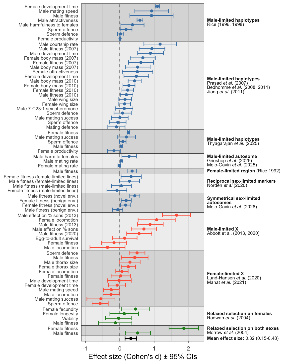
Figure 1: Forest plot showing the estimated effect sizes (Cohen’s d \(\pm\) 95% CIs). The y-axis indicates the trait being measured while horizontal grey bands show the 11 independent experimental evolution projects (projects are reported in one or more publications, named on the right). Positive effect sizes indicate evolutionary change in the direction predicted under IaSC, while negative effects indicate evolution in the opposite direction. Point colour highlights experiments using sex-limited inheritance of autosomal (blue) or X (red) genomic regions, or sex-specific relaxed selection (green). The mean effect size from meta-analysis is shown in black.
Plotting effect of moderator Generations
In short, it seems likely the negative effect of
Generations on effect size results from confounding
(i.e. the true causes are correlates of Generations, not
that variable itself).
On the right of x-axis (high generation number), this result is driven by a couple of studies, Lund-Hansen et al. (2020) and Manat et al. (2021), which both relate to the same set of experimental evolution lines, and which both focus on female-limited evolution of X chromosomes (uniquely in the full dataset). It’s possible that making the X female-limited results in less evolution than other designs, e.g. because the X is already present in females 66% of the time, though without replication this conclusion is tentative. Furthermore, we calculated the effect sizes for those 2 studies from models of their raw data, unlike for many of the studies in on the left of the x-axis (short generation number), where only summary statistics were available, which potentially inflates effect size (since it ignores details of the experimental design, incurring pseudoreplication).
library(ggrepel)
meta_analysis_data %>%
  ggplot(aes(Generations, Estimate)) +
  geom_point() +
  geom_text_repel(aes(label = Short_name), size = 2, max.overlaps = 1000)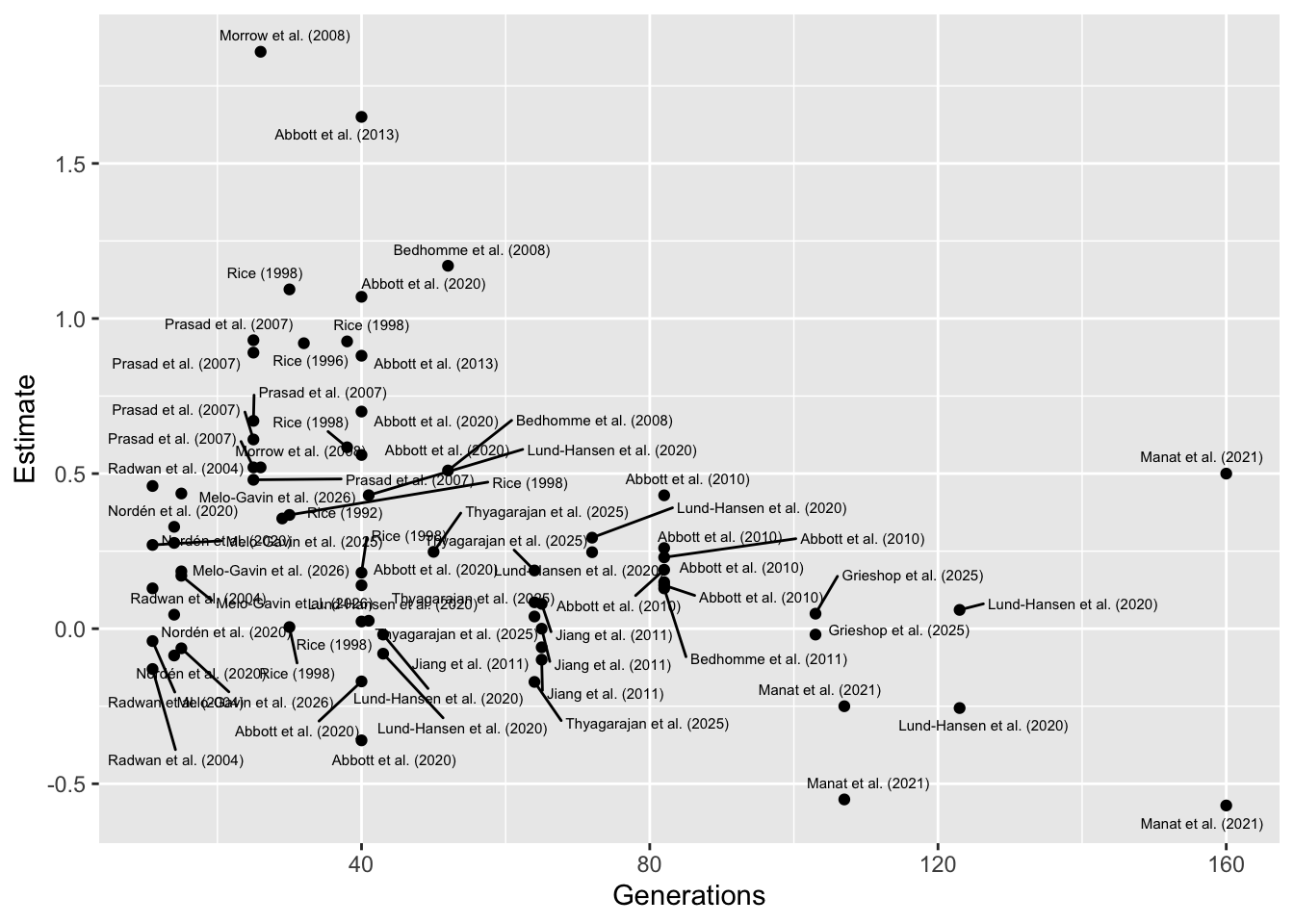
| Version | Author | Date |
|---|---|---|
| 8cb0ab7 | luekholman | 2026-03-03 |
| be1bcf7 | luekholman | 2026-03-03 |
| 8915f97 | luekholman | 2026-02-27 |
| 65e7263 | luekholman | 2026-02-27 |
| c6491af | luekholman | 2026-02-27 |
| c3874eb | luekholman | 2026-02-27 |
| 4a05564 | luekholman | 2026-02-27 |
| 8d9eb2b | luekholman | 2026-02-26 |
| f80a6dd | luekholman | 2026-02-26 |
| 0560e72 | luekholman | 2026-02-26 |
| cbdc84d | luekholman | 2026-02-25 |
| 4719bf8 | luekholman | 2026-02-20 |
| 3f80499 | luekholman | 2026-02-10 |
| f546a4c | luekholman | 2026-02-10 |
| 67d1c7a | luekholman | 2026-02-09 |
| b0251e4 | luekholman | 2026-02-09 |
| f4fb206 | luekholman | 2026-02-09 |
| 6029ddf | luekholman | 2026-02-09 |
| 7057ba1 | luekholman | 2026-02-09 |
sessionInfo()R version 4.5.2 (2025-10-31)
Platform: aarch64-apple-darwin20
Running under: macOS Tahoe 26.2
Matrix products: default
BLAS: /System/Library/Frameworks/Accelerate.framework/Versions/A/Frameworks/vecLib.framework/Versions/A/libBLAS.dylib
LAPACK: /Library/Frameworks/R.framework/Versions/4.5-arm64/Resources/lib/libRlapack.dylib; LAPACK version 3.12.1
locale:
[1] en_US.UTF-8/en_US.UTF-8/en_US.UTF-8/C/en_US.UTF-8/en_US.UTF-8
time zone: Europe/London
tzcode source: internal
attached base packages:
[1] stats graphics grDevices utils datasets methods base
other attached packages:
[1] ggrepel_0.9.6 kableExtra_1.4.0 ggh4x_0.3.1
[4] DT_0.34.0 metafor_4.8-0 numDeriv_2016.8-1.1
[7] metadat_1.4-0 Matrix_1.7-4 lubridate_1.9.4
[10] forcats_1.0.1 stringr_1.6.0 dplyr_1.2.0
[13] purrr_1.2.1 readr_2.1.6 tidyr_1.3.2
[16] tibble_3.3.1 ggplot2_4.0.2 tidyverse_2.0.0
[19] workflowr_1.7.2
loaded via a namespace (and not attached):
[1] tidyselect_1.2.1 viridisLite_0.4.2 farver_2.1.2 S7_0.2.1
[5] fastmap_1.2.0 mathjaxr_2.0-0 promises_1.5.0 digest_0.6.39
[9] timechange_0.4.0 lifecycle_1.0.5 processx_3.8.6 magrittr_2.0.4
[13] compiler_4.5.2 rlang_1.1.7 sass_0.4.10 tools_4.5.2
[17] yaml_2.3.12 knitr_1.51 labeling_0.4.3 htmlwidgets_1.6.4
[21] bit_4.6.0 xml2_1.5.2 RColorBrewer_1.1-3 withr_3.0.2
[25] grid_4.5.2 git2r_0.36.2 scales_1.4.0 cli_3.6.5
[29] rmarkdown_2.30 crayon_1.5.3 generics_0.1.4 otel_0.2.0
[33] rstudioapi_0.18.0 httr_1.4.7 tzdb_0.5.0 commonmark_2.0.0
[37] cachem_1.1.0 parallel_4.5.2 vctrs_0.7.1 jsonlite_2.0.0
[41] litedown_0.9 callr_3.7.6 hms_1.1.4 bit64_4.6.0-1
[45] systemfonts_1.3.1 crosstalk_1.2.2 jquerylib_0.1.4 glue_1.8.0
[49] ps_1.9.1 ggtext_0.1.2 stringi_1.8.7 gtable_0.3.6
[53] later_1.4.5 pillar_1.11.1 htmltools_0.5.9 R6_2.6.1
[57] textshaping_1.0.4 rprojroot_2.1.1 vroom_1.7.0 evaluate_1.0.5
[61] lattice_0.22-7 markdown_2.0 gridtext_0.1.6 httpuv_1.6.16
[65] bslib_0.10.0 Rcpp_1.1.1 svglite_2.2.2 nlme_3.1-168
[69] whisker_0.4.1 xfun_0.56 fs_1.6.6 getPass_0.2-4
[73] pkgconfig_2.0.3