Collecting primary data
Last updated: 2026-02-09
Checks: 7 0
Knit directory: exp_evol_metaanalysis/
This reproducible R Markdown analysis was created with workflowr (version 1.7.2). The Checks tab describes the reproducibility checks that were applied when the results were created. The Past versions tab lists the development history.
Great! Since the R Markdown file has been committed to the Git repository, you know the exact version of the code that produced these results.
Great job! The global environment was empty. Objects defined in the global environment can affect the analysis in your R Markdown file in unknown ways. For reproduciblity it’s best to always run the code in an empty environment.
The command set.seed(20260206) was run prior to running
the code in the R Markdown file. Setting a seed ensures that any results
that rely on randomness, e.g. subsampling or permutations, are
reproducible.
Great job! Recording the operating system, R version, and package versions is critical for reproducibility.
Nice! There were no cached chunks for this analysis, so you can be confident that you successfully produced the results during this run.
Great job! Using relative paths to the files within your workflowr project makes it easier to run your code on other machines.
Great! You are using Git for version control. Tracking code development and connecting the code version to the results is critical for reproducibility.
The results in this page were generated with repository version b0251e4. See the Past versions tab to see a history of the changes made to the R Markdown and HTML files.
Note that you need to be careful to ensure that all relevant files for
the analysis have been committed to Git prior to generating the results
(you can use wflow_publish or
wflow_git_commit). workflowr only checks the R Markdown
file, but you know if there are other scripts or data files that it
depends on. Below is the status of the Git repository when the results
were generated:
Ignored files:
    Ignored:    .DS_Store
    Ignored:    .Rproj.user/
    Ignored:    input_data/.DS_Store
    Ignored:    input_data/lundhansen_github_data_FLXevoexp-master/.DS_Store
    Ignored:    input_data/lundhansen_github_data_FLXevoexp-master/DevelopmentTimeGeneration/.Rapp.history
    Ignored:    input_data/lundhansen_github_data_FLXevoexp-master/LocomotionAssayGeneration123/.DS_Store
    Ignored:    input_data/lundhansen_github_data_FLXevoexp-master/LocomotionAssayGeneration123/.Rapp.history
    Ignored:    input_data/lundhansen_github_data_FLXevoexp-master/LocomotionAssayGeneration123/.Rhistory
    Ignored:    input_data/lundhansen_github_data_FLXevoexp-master/ReproductiveFitnessFM/.Rapp.history
    Ignored:    input_data/lundhansen_github_data_FLXevoexp-master/ReproductiveFitnessFM/.Rhistory
    Ignored:    input_data/lundhansen_github_data_FLXevoexp-master/StandardFitnessGeneration15-18/.Rapp.history
    Ignored:    input_data/lundhansen_github_data_FLXevoexp-master/StandardFitnessGeneration39-41 /.Rapp.history
    Ignored:    input_data/lundhansen_github_data_FLXevoexp-master/ThoraxSizeGeneration15-18/.Rapp.history
    Ignored:    input_data/lundhansen_github_data_FLXevoexp-master/ThoraxSizeGeneration72/.Rapp.history

Unstaged changes:
    Deleted:    data/README.md
    Deleted:    output/README.md
Note that any generated files, e.g. HTML, png, CSS, etc., are not included in this status report because it is ok for generated content to have uncommitted changes.
These are the previous versions of the repository in which changes were
made to the R Markdown (analysis/primary_data.Rmd) and HTML
(docs/primary_data.html) files. If you’ve configured a
remote Git repository (see ?wflow_git_remote), click on the
hyperlinks in the table below to view the files as they were in that
past version.
| File | Version | Author | Date | Message |
|---|---|---|---|---|
| Rmd | b0251e4 | luekholman | 2026-02-09 | Many minor edits |
| html | b0251e4 | luekholman | 2026-02-09 | Many minor edits |
| html | f4fb206 | luekholman | 2026-02-09 | First commit |
| html | f1a4d10 | luekholman | 2026-02-09 | First commit |
| html | 6029ddf | luekholman | 2026-02-09 | Build site. |
| Rmd | 7057ba1 | luekholman | 2026-02-09 | First commit |
| html | 7057ba1 | luekholman | 2026-02-09 | First commit |
library(tidyverse)
library(readxl)
library(lme4)
library(car)
library(lmerTest)
library(emmeans)
library(survival)
library(kableExtra)
library(compute.es)

# Function to parse results of compute.es::mes(), fes(), etc.
parse_es <- function(x, study, trait, generations, organism, interpretation){
  x %>%
    as.list() %>% enframe() %>% unnest(value) %>%
    filter(name %in% c("d", "var.d", "l.d", "u.d")) %>%
    mutate(type = c("Estimate", "Var", "Lower_95_CI", "Upper_95_CI")) %>%
    select(-name) %>%
    pivot_wider(names_from = type, values_from = value) %>%
    mutate(Study = study, Trait = trait, Generations = generations,
           Organism = organism, Interpretation = interpretation,
           .before = 1)
}

# Function to calculate Cohen's d effect size from a 2x2 contingency table
# It first calculates the log odds ratio, then converts this to Cohen's d via logOR * sqrt(3) / pi
# SE of the LOR is calculated using Woolf's method
get_effect_size_2x2_matrix <- function(x){

  # calculate log odds ratio as log(a*d / b*c)
  logOR <- as.numeric(log((x[1,1] * x[2,2]) /
                            (x[2,1] * x[1,2])))

  # Standard error of the log OR (Woolf method)
  SE_logOR <- 1/x[1,1] + 1/x[1,2] + 1/x[2,1] + 1/x[2,2]

  # 95% CIs of the log OR
  CI_logOR <- logOR + c(-1, 1) * 1.96 *  SE_logOR

  # Convert LOR to d:
  d <- logOR * sqrt(3) / pi
  SE_d <- SE_logOR * sqrt(3) / pi
  CI_d <- CI_logOR * sqrt(3) / pi

  tibble(Estimate = d,
         Var = SE_d ^ 2,
         Lower_95_CI = CI_d[1],
         Upper_95_CI = CI_d[2])
}
Overview
Cohen’s \(d\)
This document describes how I estimated Cohen’s \(d\) for each primary study in the meta-analysis. Cohen’s \(d\) is a standardised measure of the effect size, defined as the difference between two means, expressed in standard deviations of the variable of interest. Conventionally, Cohen’s \(d > |0.5|\) is considered a ‘large’ effect.
Meaning of effect size sign
Crucially, effect sizes have a sign (positive or negative, depending on whether mean 1 or mean 2 is the larger) as well as a magnitude. Unlike the magnitude, the sign is determined solely by the researcher: it depends on which of the two means is designated as the reference for comparison.
To ensure the effect size sign is meaningful and comparable across studies, I defined a positive effect size to indicate that the two means differ in the direction that one would predict if intralocus sexual conflict is present, and a negative effect to mean that the means differ in a direction opposite to this prediction.
For example, for a study like Prasad et al. (2007) that removed selection on females and then measured mean male and female fitness relative to a control, we would predict male-evolved populations to have higher male fitness and lower female fitness if intralocus sexual conflict is present. So, a positive effect size should indicate higher male fitness but lower female fitness in the experimental group relative to the control. This is potentially confusing, but it ensures that finding the mean effect size via meta-analysis is useful: a positive mean effect size would mean that experimental evolution studies tend to produce the results predicted if IaSC is common.
To clarify the meaning of each effect size, I provide a column called ‘interpretation’ in the final table of effect sizes, and document the more confusing/ambiguous decisions in this document below.
How Cohen’s \(d\) was calculated
Preferred method: from the raw data
If the primary study’s raw data were available (e.g. on Dryad or Figshare, or as a table in the original paper), I calculated the effect size from an appropriate statistical model that accounted for the structure of the experimental design (e.g. the use of replicate experimental evolution lines), block effects, etc. (following the model used by the original authors wherever possible). The models chosen are documented in the code below.
For response variables where it was appropriate to use Gaussian linear (mixed) models, I first transformed the response variable to have a mean of zero and variance of 1, such that the difference between treatment means estimates by the statistical model is equal to Cohen’s d.
For generalised (e.g. binomial) models that estimated treatment means as a log odds ratio (\(\log(\mathrm{OR})\)), or a log hazard ratio (for survival models), I converted this effect size to Cohen’s d using the standard approximation:
\(\log(\mathrm{OR}) = \frac{\sqrt{3}}{\pi}\)
For studies where the original data represent counts of binary events tallied up in a \(2\times2\) contingency table (e.g. number of surviving and non-surviving individuals from the treatment and control groups) with elements \(a\),\(b\),\(c\) and \(d\), I estimated the log odds ratio as \(log(a\times d / b\times c)\) and found the SE of the log odds ratio using Woolf’s method, i.e.
\[SE\!\left(\log(\mathrm{OR})\right) =\sqrt{\frac{1}{a}+\frac{1}{b}+\frac{1}{c}+\frac{1}{d}}\]
Fall-back method: from the group means
For many studies, the raw data were not available, but the paper
provided numerical or graphical information about 1) the means of each
treatment group, 2) either the group standard deviations or the standard
errors of the means (which allow calculation of the standard deviation
as \(SD = SE\times\sqrt{N}\)), and 3)
the sample size N. From these three quantities, one can estimate Cohen’s
d (I used the function mes() from the
compute.es package). Where possible I obtained these
numbers from tables or the main text, but often the data were only
contained in figures (e.g. bar charts showing the mean and standard
errors). In the latter case, I measured the means and standard errors
using the web application PlotDigitizer - this data
extraction step is expected to add inaccuracy, but not to add consistent
bias.
Using group means is a less accurate method because it is not possible to account for the structure of the experimental design, incurring pseudoreplication. For example, in studies where the authors had 4 replicate experimental evolution lines for 2 treatments and measured 20 individuals per line, the sample size is not really 80 per treatment, since there are 20 replicate measurements of only 8 lines. This will make the effect size measurements appear more precise than they should be, giving extra weight to those studies in the meta-analysis.
Workflow in the code below
For each publication, I either load or type out the raw data, display it (in cases where I extracted the raw data or group means from the primary paper), calculate effect size, and then save it to a small .csv file along with meta-data like the paper of origin, the trait being measured, the number of generations of selection prior to measuring the trait, and a plain English interpretation of the meaning of the effect size (e.g. that the trait is higher/lower in one treatment group compared to another such group).
Sex-limited evolution experiments
This section covers publications that evolved genomic elements (e.g. small regions or whole chromosomes) mostly/entirely within one sex for multiple generations. In general, I predict that this treatment will increase fitness in that sex, reduce fitness in the other sex, and cause phenotypic evolution towards the typical trait values for the evolving sex (e.g. in Drosophila, chromosomes that had undergone male-limited evolution in should encode smaller body size and slower development time). The effect size signs selected reflect these expectations.
Rice (1992)
Rice, W. R. (1992). Sexually antagonistic genes: experimental evidence. Science, 256, 1436-1439.
Rice’s original data
These data are shown in Table 1. Letters R, P, S and O denote the 4 eye colours of males that females might mate to, where O (orange-eyed) represents non-focal males and R/P/S are the focal male (which differ in how many copies of the evolved genomic region is carried). The focal males carry alleles from either the control or the population undergoing female-limited evolution of a small genomic region. The R,P,S, and O columns are percentages, with the last column giving the total number of females tested.
df <- tibble(
  replicate = c(1,2,1,2),
  treatment = c("control", "control", "experimental", "experimental"),
  R = c(42, 36, 40, 17),
  P = c(26, 21, 20, 40),
  S = c(22, 33, 22, 26),
  O = c(10, 9, 17, 17),
  total = c(90, 75, 90, 70)
)

df %>%
  kable() %>%
kable_styling()| replicate | treatment | R | P | S | O | total |
|---|---|---|---|---|---|---|
| 1 | control | 42 | 26 | 22 | 10 | 90 |
| 2 | control | 36 | 21 | 33 | 9 | 75 |
| 1 | experimental | 40 | 20 | 22 | 17 | 90 |
| 2 | experimental | 17 | 40 | 26 | 17 | 70 |
Calculating effect size
# first convert the 4 percentage columns to counts of females (with rounding)
df$R <- round((df$R/100) * df$total)
df$P <- round((df$P/100) * df$total)
df$S <- round((df$S/100) * df$total)
df$O <- round((df$O/100) * df$total)

# Pool the females over the 3 types representing focal males
focal_male_chosen <- rowSums(df %>% select(R, P, S))

# Make a 2x2 contingency table giving number of times the focal vs non-focal male mated, for control vs experimental
x <- matrix(c(focal_male_chosen[1] + focal_male_chosen[2],
         focal_male_chosen[3] + focal_male_chosen[4],
         df$O[1] + df$O[2],
         df$O[3] + df$O[4]), ncol = 2)

get_effect_size_2x2_matrix(x) %>%
    mutate(Study = "Rice (1992) Science 256, 1436-1439",
           Trait = "Male fitness",
           Generations = "29",
           Organism = "Drosophila melanogaster",
           Interpretation = "A positive effect size means that males carrying a genomic region that underwent female-limited evolution had lower fitness compared to males carrying control genomes.",
           .before = 1) %>%
  write_csv("effect_sizes/rice92.csv")
Rice (1996)
Rice, W. R. (1996). Sexually antagonistic male adaptation triggered by experimental arrest of female evolution. Nature, 381, 232–234.
Male fitness
Rice’s original data
The means for the male fitness were recorded from Figure 1, using PlotDigitizer.
# These data come from using PlotDigitizer web app on data in the first 2 columns of Figure 2
rice96 <- tibble(generation = c(rep(31,4), rep(32, 4)),
       replicate = rep(c("A", "A", "B", "B"), 2),
       treatment = rep(c("ML", "Control", "ML", "Control"), 2),
       fitness = c(1.312563038, 1.040288341, 1.240486316, 0.959122165,
                   1.233782098, 1.018216389, 1.182082107, 0.982122656),
       sample_size = rep(c(4,8), each=4))

rice96 %>%
  mutate(fitness = round(fitness,2)) %>%
  rename(`Male fitness` = fitness) %>%
kable() %>% kable_styling(full_width = F)| generation | replicate | treatment | Male fitness | sample_size |
|---|---|---|---|---|
| 31 | A | ML | 1.31 | 4 |
| 31 | A | Control | 1.04 | 4 |
| 31 | B | ML | 1.24 | 4 |
| 31 | B | Control | 0.96 | 4 |
| 32 | A | ML | 1.23 | 8 |
| 32 | A | Control | 1.02 | 8 |
| 32 | B | ML | 1.18 | 8 |
| 32 | B | Control | 0.98 | 8 |
Calculating effect size
Unfortunately the study provides means but no standard error or standard deviation, which we need to compute effect size variance and confidence limits.
To get an estimate of effect size, we assume here the standard deviation (SD) is the same as the SD in similar male fitness assays carried out in Wong & Holman (2023; Evolution). That study’s male fitness assay methods were quite similar, and focused on North American D. melanogaster as well. We load that study’s raw data, and find the average standard deviation in proportion of offspring sired relative to competitor males. We then use simulation to generate 10,000 possible datasets for Rice (1996) by generating random Normally distributed numbers using the means from Rice’s Figure 1 and SD for Wong & Holman, and from these random datasets calculate 10,000 estimates of the standardised effect size Cohen’s d comparing the two treatments. From these 10,000 estimates we also obtain the effect size variance and 95% CIs.
# Rice's description of the male fitness trait:
# Extra vials were constructed by mixing EA, EB, CA', and CB' males with target females (4 and 8 vials each in generations 31 and 32, respectively) using a procedure matching that of the adapting-male compartment of Fig. 1, except that 75% of the males were replaced by competitor males that were homozygous for the marker pP (previously recombined into the genetic background of the LH source stock). Offspring from competitor males were pink-eyed and could be distinguished from red-eyed males carrying the genomic haplotype of the experimental (EA or EB) or control (CA' or CB') males. The ratio of red-eyed to pink-eyed adult male offspring, after adjusting for Mendelian segregation, measured net relative fitness.

# Find the standard deviation in proportion offspring sired in a different study, Wong & Holman 2023 Evolution, for 810 male fitness assays covering 125 fly genotypes
# Then take the average SD across those 125 genotypes, and assume this is representative of the SD in Rice's study
estimated_SD <- read_csv(
  "input_data/male_fitness_raw_data_wong_and_holman.csv",
  show_col_types = FALSE) %>%
  mutate(fitness = `Early male focal` /
           (`Early male focal` + `Early male rival`)) %>%
  group_by(Line) %>%
  summarise(mean_fitness = mean(fitness),
            sd_fitness = sd(fitness)) %>%
  summarise(x = mean(sd_fitness, na.rm=T)) %>% pull(x)


# make n random normal fitness values given mean and SD
make_data <- function(mean_fitness, n, sd){
  rnorm(n, mean_fitness, sd)
}

bootstrapped_effect_sizes <- lapply(1:1000, function(i){

  possible_dataset <- map_df(1:8, ~ tibble(
    generation = rice96$generation[.x],
    replicate = rice96$replicate[.x],
    treatment = rice96$treatment[.x],
    fitness = rnorm(n = rice96$sample_size[.x],
                    mean = rice96$fitness[.x],
                    sd = estimated_SD))) %>%
    mutate(line = paste(treatment, replicate, sep = "_"),
           fitness = as.numeric(scale(fitness))) # scale fitness

  # do a linear model (effect size of treatment is equal to Cohen's d)
  as.numeric(summary(lm(fitness ~ treatment + line, data = possible_dataset))$coefficients[2,1:2])
}) %>%
  do.call("rbind", .) %>%
  as.data.frame() %>% as_tibble() %>%
  mutate(V2 = V2 ^ 2) %>% # Square the effect size SE to get the variance
  rename(Estimate = V1, Var = V2)

bootstrapped_effect_sizes %>%
  summarise(Estimate = mean(Estimate), # bootstrapped Cohen's d effect size
            Var = mean(Var)) %>%       # bootstrapped variance in Cohen's d effect size
  mutate(Lower_95_CI = Estimate - 1.96 * sqrt(Var),
         Upper_95_CI = Estimate + 1.96 * sqrt(Var)) %>%
    mutate(Study = "Rice (1996) Nature 381, 232–234",
           Trait = "Male fitness",
           Generations = "32",
           Organism = "Drosophila melanogaster",
           Interpretation = "The positive effect size means that males carrying a genomic region that underwent male-limited evolution had higher fitness than males carrying control genomes",
           .before = 1)  %>%
  write_csv("effect_sizes/rice96.csv")
Rice (1998)
Rice, W. R. (1998). Male fitness increases when females are eliminated from the gene pool: Implications for the Y chromosome. PNAS, 95, 6217–6221.
Mating speed
Data obtained from Figure 1A, using PlotDigitiser. Rice placed males with male-evolved or control genomes in vials with virgin females, and counted the number of mating pairs after 15 minutes. This is a rough measure of how quickly males induce virgin females to mate and presumably correlates with males’ ability to find/court females, attractiveness and mating duration.
Rice’s original data
x <- matrix(c(52, 3, 42, 13), nrow = 2)
colnames(x) <- c("male-limited", "control")
rownames(x) <- c("mated", "unmated")
kable(x) %>% kable_styling(full_width = F)| male-limited | control | |
|---|---|---|
| mated | 52 | 42 |
| unmated | 3 | 13 |
Calculating effect size
get_effect_size_2x2_matrix(x) %>%
    mutate(Study = "Rice (1998) PNAS, 95, 6217–6221",
           Trait = "Male mating speed",
           Generations = "38",
           Organism = "Drosophila melanogaster",
           Interpretation = "The positive effect size means that males carrying a haplotype that underwent male-limited evolution mated with previously-unmated females faster than males carrying control haplotypes",
           .before = 1) %>%
  write_csv("effect_sizes/rice98_1.csv")
Male attractiveness to mated females
This data is from Figure 1B (early measure), and shows the number of female flies mating vs not-mating with either EAB or CAB males. More females remating implies that the male type is better able to achieve matings with mated females (who recently mated with another male, of the same type as the focal male). Females remated more with EAB males than CAB males.
Rice’s raw data
x <- matrix(c(54, 25, 140-54, 140-25), nrow=2)
colnames(x) <- c("n_remating", "n_not_remating")
rownames(x) <- c("EAB", "CAB")
kable(x) %>% kable_styling(full_width = F)| n_remating | n_not_remating | |
|---|---|---|
| EAB | 54 | 86 |
| CAB | 25 | 115 |
Effect size
get_effect_size_2x2_matrix(x) %>%
    mutate(Study = "Rice (1998) PNAS, 95, 6217–6221",
           Trait = "Male attractiveness to mated females",
           Generations = "38",
           Organism = "Drosophila melanogaster",
           Interpretation = "The positive effect size means that males carrying a haplotype that underwent male-limited evolution attained more matings with previously-mated females compared to males carrying control haplotypes",
           .before = 1) %>%
  write_csv("effect_sizes/rice98_2.csv")
Sperm defence
Data collected from Figure 1C using PlotDigitiser. The data shows the proportion sired by the focal male (which carried either EAB or CAB genomes) after the female mated to a second male of a standard genoptype carrying marker mutations. Higher values indicate better ‘sperm defence’, i.e. reduced paternity loss to the second male.
Rice’s raw data
m <- as.data.frame(matrix(
  c(
    0.8087228560912771, 13.078892347721043,
    1.1769782848730217, 15.50243925103378,
    1.826647037173353, 23.728290665799378,
    2.1877806404122193, 19.96520001858477,
    2.8175193227824806, 19.078474190400968,
    3.191001104158999, 19.057008781303722,
    3.830622009569378, 49.462760767550996,
    4.195491350754509, 49.75561027737769),
  ncol = 2,
  byrow = TRUE)) %>%
  mutate(treatment = rep(c("EAB", "CAB"), 4),
         type = rep(c("all_pink", "most_pink", "most_red", "all_red"), each=2),
         n = round(V2)) %>% select(treatment, type, n)

kable(m) %>% kable_styling(full_width = F)| treatment | type | n |
|---|---|---|
| EAB | all_pink | 13 |
| CAB | all_pink | 16 |
| EAB | most_pink | 24 |
| CAB | most_pink | 20 |
| EAB | most_red | 19 |
| CAB | most_red | 19 |
| EAB | all_red | 49 |
| CAB | all_red | 50 |
Effect size
To get a Cohen’s d effect size, I first reduce the results from a 4x2 contingency table to a 2x2 one, by pooling the all-red and mostly-red categories, and the all-pink and mostly-pink categories. A positive effect size here would mean better sperm defence in EAB males than CAB (though the effect size does not differ significantly from zero).
x <- matrix(c(m$n[1] + m$n[3],
         m$n[2] + m$n[4],
         m$n[5] + m$n[7],
         m$n[6] + m$n[8]), nrow = 2)

get_effect_size_2x2_matrix(x) %>%
    mutate(Study = "Rice (1998) PNAS, 95, 6217–6221",
           Trait = "Male sperm defence",
           Generations = "40",
           Organism = "Drosophila melanogaster",
           Interpretation = "A positive effect size means that males carrying a haplotype that underwent male-limited evolution fertilise more offspring when mating first in twice-mated females, compared to males carrying control haplotypes (though there is no significant difference between the two treatments)",
           .before = 1) %>%
  write_csv("effect_sizes/rice98_3.csv")
Sperm offence
Data collected from Figure 1D using PlotDigitiser. Rice mated females to a pink-eyed male first, then put them with a tester EAB or CAB male, and recorded the progeny genotypes qualitatively (mostly- or all-red vs pink). He reports a significant difference using a “directed \(\chi^2\) contingency test” (perhaps meaning a 1-tail test), but the result appears non-significant with a standard 2-tailed test.
Rice’s raw data
m <- as.data.frame(matrix(
  c(
    0.8123905550128108, 10.75088339222615,
    1.1750935466627344, 16.231552691748078,
    1.8095150319809772, 2.1388484722510914,
    2.169287202079224, 0.6308459779671587,
    2.7968885366168363, 11.076699230929123,
    3.1919042966949918, 21.357825815838705,
    3.8175517501981533, 76.27520266056953,
    4.176346979779175, 61.42434005404282
  ),
  ncol = 2,
  byrow = TRUE
)) %>%
  mutate(treatment = rep(c("EAB", "CAB"), 4),
         type = rep(c("all_pink", "most_pink", "most_red", "all_red"), each=2),
         n = round(V2)) %>% select(treatment, type, n)

m %>%
  pivot_wider(names_from = type, values_from = n) %>%
  kable() %>%
kable_styling(full_width = F)| treatment | all_pink | most_pink | most_red | all_red |
|---|---|---|---|---|
| EAB | 11 | 2 | 11 | 76 |
| CAB | 16 | 1 | 21 | 61 |
Effect size
To get a Cohen’s d effect size, I first reduce the results from a 4x2 contingency table to a 2x2 one, by pooling the all-red and mostly-red categories, and the all-pink and mostly-pink categories. A positive effect size here would mean better sperm offence in EAB males than CAB (though the effect size does not differ significantly from zero).
x <- matrix(c(m$n[5] + m$n[7],
         m$n[6] + m$n[8],
         m$n[1] + m$n[3],
         m$n[2] + m$n[4]), nrow = 2)

# positive effect means higher sperm offence for EAB males. It is not significant, contra Rice's analysis
get_effect_size_2x2_matrix(x) %>%
    mutate(Study = "Rice (1998) PNAS, 95, 6217–6221",
           Trait = "Male sperm offence",
           Generations = "40",
           Organism = "Drosophila melanogaster",
           Interpretation = "A positive effect size means that males carrying a haplotype that underwent male-limited evolution fertilise more offspring when mating second in twice-mated females, compared to males carrying control haplotypes (though there is no significant difference between the two treatments)",
           .before = 1) %>%
  write_csv("effect_sizes/rice98_4.csv")
Sex-specific development time
Rice’s original data
These data were extracted from Figure 2A using PlotDigitizer. The data show the numbers of females eclosed in each of the 4 replicate lines over a few days. We do not know what fraction of eggs hatched, so this data tells us only the development time of females who eventually hatched. It’s also unclear if more females would have hatched on later days.
Additionally, Rice does not present data on male development time for the other half of this progeny pool. I assume these data would have been collected, since Rice would have had to sex the flies to find all these females and could have easily counted the pile of males as well, so I do wonder if these results were left out since they were not significant in the predicted direction (i.e. masculinised, longer development in male EAB flies).
dt <- read_csv("input_data/rice98_development_time.csv",
               show_col_types = F) %>%
  mutate(n_females_emerged = round(prop_emerged * overall_eclosed),
         n_females_not_emerged = overall_eclosed - n_females_emerged) %>%
  mutate(treatment = substr(population, 1, 1),
         line = population, .before = 1,
         replicate = paste(population, generation, sep = "_"),
         day_centered = as.numeric(scale(day))) # mean-centre day and scale by dividing by its SD

kable(dt) %>% kable_styling()| treatment | line | replicate | day_centered | day | prop_emerged | overall_eclosed | population | generation | n_females_emerged | n_females_not_emerged |
|---|---|---|---|---|---|---|---|---|---|---|
| C | CA | CA_29 | -1.2789518 | 10.0 | 0.5311097 | 114 | CA | 29 | 61 | 53 |
| C | CA | CA_29 | -0.8275571 | 10.5 | 0.5926928 | 114 | CA | 29 | 68 | 46 |
| C | CA | CA_29 | -0.3761623 | 11.0 | 0.7550655 | 114 | CA | 29 | 86 | 28 |
| C | CA | CA_29 | 0.0752325 | 11.5 | 0.9427559 | 114 | CA | 29 | 107 | 7 |
| C | CA | CA_29 | 0.5266272 | 12.0 | 0.9972443 | 114 | CA | 29 | 114 | 0 |
| C | CA | CA_29 | 1.4294167 | 13.0 | 1.0000000 | 114 | CA | 29 | 114 | 0 |
| C | CB | CB_29 | -1.2789518 | 10.0 | 0.4769470 | 126 | CB | 29 | 60 | 66 |
| C | CB | CB_29 | -0.8275571 | 10.5 | 0.5371122 | 126 | CB | 29 | 68 | 58 |
| C | CB | CB_29 | -0.3761623 | 11.0 | 0.7500050 | 126 | CB | 29 | 95 | 31 |
| C | CB | CB_29 | 0.0752325 | 11.5 | 0.8978175 | 126 | CB | 29 | 113 | 13 |
| C | CB | CB_29 | 0.5266272 | 12.0 | 0.9863767 | 126 | CB | 29 | 124 | 2 |
| C | CB | CB_29 | 1.4294167 | 13.0 | 1.0000000 | 126 | CB | 29 | 126 | 0 |
| E | EA | EA_29 | -1.2789518 | 10.0 | 0.2708133 | 126 | EA | 29 | 34 | 92 |
| E | EA | EA_29 | -0.8275571 | 10.5 | 0.3939294 | 107 | EA | 29 | 42 | 65 |
| E | EA | EA_29 | -0.3761623 | 11.0 | 0.7496843 | 107 | EA | 29 | 80 | 27 |
| E | EA | EA_29 | 0.0752325 | 11.5 | 0.9169923 | 107 | EA | 29 | 98 | 9 |
| E | EA | EA_29 | 0.5266272 | 12.0 | 0.9739658 | 107 | EA | 29 | 104 | 3 |
| E | EA | EA_29 | 1.4294167 | 13.0 | 1.0000000 | 107 | EA | 29 | 107 | 0 |
| E | EB | EB_29 | -1.2789518 | 10.0 | 0.1981622 | 103 | EB | 29 | 20 | 83 |
| E | EB | EB_29 | -0.8275571 | 10.5 | 0.3488406 | 103 | EB | 29 | 36 | 67 |
| E | EB | EB_29 | -0.3761623 | 11.0 | 0.6018468 | 103 | EB | 29 | 62 | 41 |
| E | EB | EB_29 | 0.0752325 | 11.5 | 0.7704475 | 103 | EB | 29 | 79 | 24 |
| E | EB | EB_29 | 0.5266272 | 12.0 | 0.9747725 | 103 | EB | 29 | 100 | 3 |
| E | EB | EB_29 | 1.4294167 | 13.0 | 1.0000000 | 103 | EB | 29 | 103 | 0 |
| C | CA | CA_30 | -1.2789518 | 10.0 | 0.3810871 | 141 | CA | 30 | 54 | 87 |
| C | CA | CA_30 | -0.8275571 | 10.5 | 0.5640077 | 141 | CA | 30 | 80 | 61 |
| C | CA | CA_30 | -0.3761623 | 11.0 | 0.7751702 | 141 | CA | 30 | 109 | 32 |
| C | CA | CA_30 | 0.0752325 | 11.5 | 0.9135555 | 141 | CA | 30 | 129 | 12 |
| C | CA | CA_30 | 0.9780220 | 12.5 | 0.9889588 | 141 | CA | 30 | 139 | 2 |
| C | CA | CA_30 | 1.8808115 | 13.5 | 1.0000000 | 141 | CA | 30 | 141 | 0 |
| C | CB | CB_30 | -1.2789518 | 10.0 | 0.4061285 | 148 | CB | 30 | 60 | 88 |
| C | CB | CB_30 | -0.8275571 | 10.5 | 0.5808272 | 148 | CB | 30 | 86 | 62 |
| C | CB | CB_30 | -0.3761623 | 11.0 | 0.7250661 | 148 | CB | 30 | 107 | 41 |
| C | CB | CB_30 | 0.0752325 | 11.5 | 0.8855230 | 148 | CB | 30 | 131 | 17 |
| C | CB | CB_30 | 0.9780220 | 12.5 | 0.9622366 | 148 | CB | 30 | 142 | 6 |
| C | CB | CB_30 | 1.8808115 | 13.5 | 1.0000000 | 148 | CB | 30 | 148 | 0 |
| E | EA | EA_30 | -1.2789518 | 10.0 | 0.2168442 | 143 | EA | 30 | 31 | 112 |
| E | EA | EA_30 | -0.8275571 | 10.5 | 0.3997003 | 143 | EA | 30 | 57 | 86 |
| E | EA | EA_30 | -0.3761623 | 11.0 | 0.6844457 | 143 | EA | 30 | 98 | 45 |
| E | EA | EA_30 | 0.0752325 | 11.5 | 0.8648744 | 143 | EA | 30 | 124 | 19 |
| E | EA | EA_30 | 0.9780220 | 12.5 | 0.9621721 | 143 | EA | 30 | 138 | 5 |
| E | EA | EA_30 | 1.8808115 | 13.5 | 1.0000000 | 143 | EA | 30 | 143 | 0 |
| E | EB | EB_30 | -1.2789518 | 10.0 | 0.2600960 | 153 | EB | 30 | 40 | 113 |
| E | EB | EB_30 | -0.8275571 | 10.5 | 0.4234797 | 153 | EB | 30 | 65 | 88 |
| E | EB | EB_30 | -0.3761623 | 11.0 | 0.6160398 | 153 | EB | 30 | 94 | 59 |
| E | EB | EB_30 | 0.0752325 | 11.5 | 0.7607297 | 153 | EB | 30 | 116 | 37 |
| E | EB | EB_30 | 0.9780220 | 12.5 | 0.8687464 | 153 | EB | 30 | 133 | 20 |
| E | EB | EB_30 | 1.8808115 | 13.5 | 1.0000000 | 153 | EB | 30 | 153 | 0 |
Calculating effect size
Here, I fit a binomial GLMM using the lme4 package with the form
\[Y = day \times treatment + (1 | line)\]
With Y being a 2-column response variable giving the number of females eclosed or not yet eclosed, day in standard units, treatment being male-limited or control, and line being a 4-level factor (2 replicate lines each of the 2 treatments).
I then used the fitted model to estimate the expected day on which 50% of the females had eclosed for each treatment, and used parametric bootstrapping to find the difference in number of days between the treatments (i.e. Cohen’s d since day was standardised).
The positive effect size indicates slower emergence of females carrying male-limited genomes (i.e. masculinisation of the phenotype). Rice interprets this result as extra female-harming mutations accumulating under male-limited selection, which is an additional valid interpretation.
resp <- with(dt, cbind(n_females_emerged, n_females_not_emerged))
model <- glmer(
  resp ~ day_centered + treatment + (1 | line),
  family = binomial,
  data = dt,
  control = glmerControl(optimizer = "bobyqa")
)

# Get the log odds ratio effect size (+ SE) of treatment on Prob(eclosion) at the average value of day (i.e. day = 11.42)
LOR <- coef(summary(model))[2,1:2] %>% as.numeric()


tibble(
  Estimate = LOR[1] * sqrt(3) / pi,
  Var = (LOR[2]^2) * sqrt(3) / pi,
  Lower_95_CI = (LOR[1] - LOR[2]*1.96) * sqrt(3) / pi,
  Upper_95_CI = (LOR[1] + LOR[2]*1.96) * sqrt(3) / pi) %>%
    mutate(Study = "Rice (1998) PNAS, 95, 6217–6221",
           Trait = "Female development time",
           Generations = "30",
           Organism = "Drosophila melanogaster",
           Interpretation = "The positive effect size means females carrying haplotypes that underwent male-limited evolution took longer to complete development than females carrying control genomes.",
           .before = 1) %>%
  write_csv("effect_sizes/rice98_5.csv")
Female productivity
The data are from Figure 2B (captured with PlotDigitizer). Rice counted the “total number of adult offspring (measures net female fitness independent of development time) produced by EAB or CAB females (red-eyed offspring) in competition with tester-females (pink-eyed offspring).” There was no difference, implying that EAB and CAB are equally good at producing eggs and their offspring have equal survival rates (or if there are differences in these fitness components, then they cancel out). Note that in the methods and the figure axis label, Rice mentions that he only counted the daughters, while in the figure caption (quoted here) he says that all offspring were counted (meaning, sons too). It’s unclear which was measured, but it likely does not qualitatively change the result.
Rice’s original data
x <- matrix(c(349, 344, 197, 196), nrow = 2)
colnames(x) <- c("focal_female_offspring", "rival_female_offspring")
rownames(x) <- c("CAB", "EAB")

kable(x) %>% kable_styling(full_width = F)| focal_female_offspring | rival_female_offspring | |
|---|---|---|
| CAB | 349 | 197 |
| EAB | 344 | 196 |
Calculating effect size
Here, we define a positive effect to mean that EAB females are less productive (which is what we’d predict if male-limited selection harms female fitness), though the observed effect size is zero or close to it.
get_effect_size_2x2_matrix(x) %>%
    mutate(Study = "Rice (1998) PNAS, 95, 6217–6221",
           Trait = "Female productivity",
           Generations = "30",
           Organism = "Drosophila melanogaster",
           Interpretation = "A positive effect size means that females carrying a haplotype that underwent male-limited evolution produced fewer offspring than females carrying a control haplotype (though there is no significant difference).",
           .before = 1) %>%
  write_csv("effect_sizes/rice98_6.csv")
Mortality of males’ mates
Rice’s original data
Data extracted from Figure 3A with PlotDigitizer.
mortality <- tibble(
  treatment = rep(c("EAB", "CAB"), each = 7),
  day = c(
    0,1,2,3,4,5,12, 0,1,2,3,4,5,12),
  n_dead_females = c(
    0,4,7,8,9,15,29,0,0,2,2,2,5,16),
  n_live_females = 140 - n_dead_females)

kable(mortality) %>%
kable_styling(full_width = F)| treatment | day | n_dead_females | n_live_females |
|---|---|---|---|
| EAB | 0 | 0 | 140 |
| EAB | 1 | 4 | 136 |
| EAB | 2 | 7 | 133 |
| EAB | 3 | 8 | 132 |
| EAB | 4 | 9 | 131 |
| EAB | 5 | 15 | 125 |
| EAB | 12 | 29 | 111 |
| CAB | 0 | 0 | 140 |
| CAB | 1 | 0 | 140 |
| CAB | 2 | 2 | 138 |
| CAB | 3 | 2 | 138 |
| CAB | 4 | 2 | 138 |
| CAB | 5 | 5 | 135 |
| CAB | 12 | 16 | 124 |
Calculating effect size
To calculate the effect size, I fit a Cox’s proportional hazard model to the female surivivorship data, and measured the difference between the male-limited and control treatments in the per-day risk of death (conditional on being alive), taking into account the right censoring of the data (since the experiment ended on day 15, when most females were still alive). There is a weakly significant difference, such that females die faster when mated to EAB males, which is qualitatively the same conclusion Rice reached (Rice used several pairwise t-tests to test specific days one-at-a-time, which is a weaker approach, but understandable given the statistical software available in 1998).
The positive effect size means that females die faster when mated to males carrying male-evolved compared to control genomes.
make_surv_data <- function(day, cum_dead, treatment) {
  new_deaths <- c(cum_dead[1], diff(cum_dead))
  death_times <- rep(day, new_deaths)
  data.frame(
    time = death_times,
    event = 1,
    treatment = treatment
  )
}

surv_A <- make_surv_data(
  day = mortality$day[mortality$treatment == "EAB"],
  cum_dead = mortality$n_dead_females[mortality$treatment == "EAB"],
  treatment = "EAB"
)

surv_B <- make_surv_data(
  day = mortality$day[mortality$treatment == "CAB"],
  cum_dead = mortality$n_dead_females[mortality$treatment == "CAB"],
  treatment = "CAB"
)

surv_data <- bind_rows(surv_A, surv_B)

censored_A <- data.frame(
  time = 12,
  event = 0,
  treatment = "EAB"
)[rep(1, 140 - nrow(surv_A)), ]

censored_B <- data.frame(
  time = 12,
  event = 0,
  treatment = "CAB"
)[rep(1, 140 - nrow(surv_B)), ]

surv_data <- bind_rows(surv_data, censored_A, censored_B)

cox <- coxph(
  Surv(time, event) ~ treatment,
  data = surv_data
)

logHR <- coef(cox)["treatmentEAB"]
Var_HR <- vcov(cox)["treatmentEAB", "treatmentEAB"]
CI_logHR <- logHR + c(-1, 1) * 1.96 * sqrt(Var_HR)

d <- logHR * sqrt(3) / pi
Var_d <- Var_HR * sqrt(3) / pi
CI_d <- CI_logHR * sqrt(3) / pi

tibble(
  Estimate = d,
  Var = Var_d,
  Lower_95_CI = CI_d[1],
  Upper_95_CI = CI_d[2]) %>%
    mutate(Study = "Rice (1998) PNAS, 95, 6217–6221",
           Trait = "Male harmfulness to females",
           Generations = "30",
           Organism = "Drosophila melanogaster",
           Interpretation = "A positive effect size means that males carrying a haplotype that underwent male-limited evolution have a negative effect on the survival of their mates.",
           .before = 1) %>%
  write_csv("effect_sizes/rice98_7.csv")
Prasad et al. (2008)
Prasad, N. G., Bedhomme, S., Day, T., & Chippindale, A. K. (2007). An evolutionary cost of separate genders revealed by male-limited evolution. The American Naturalist, 169, 29–37.
Male and female fitness
Prasad et al.’s original data
The data come from Figure 2 (transcribed with PlotDigitizer).
df <- data.frame(
  treatment = c(
    "control","control", "male_evolved", "male_evolved"),
  sex = c(
    "female","male","female","male"),
  mean = c(
    0.858247281,0.73376332,0.785461824,0.845795256),
  SE = c(
    0.015168311,0.015320071,0.015529016,0.015670879
  )
)

kable(df) %>%
kable_styling(full_width = F)| treatment | sex | mean | SE |
|---|---|---|---|
| control | female | 0.8582473 | 0.0151683 |
| control | male | 0.7337633 | 0.0153201 |
| male_evolved | female | 0.7854618 | 0.0155290 |
| male_evolved | male | 0.8457953 | 0.0156709 |
Calculating effect size
The effect size was calculated from the means and standard errors for each treatment, separately for both male fitness and female fitness.
# mes(m.1 = df$mean[df$treatment == "control" & df$sex == "female"],
#     m.2 = df$mean[df$treatment == "male_evolved" & df$sex == "female"],
#     sd.1 = df$SE[df$treatment == "control" & df$sex == "female"] * sqrt(15),
#     sd.2 = df$SE[df$treatment == "male_evolved" & df$sex == "female"] * sqrt(15),
#     n.1 = 15, n.2 = 15, verbose=F) %>%
#   parse_es()
#
# mes(m.1 = df$mean[df$treatment == "control" & df$sex == "male"],
#     m.2 = df$mean[df$treatment == "male_evolved" & df$sex == "male"],
#     sd.1 = df$SE[df$treatment == "control" & df$sex == "male"] * sqrt(15),
#     sd.2 = df$SE[df$treatment == "male_evolved" & df$sex == "male"] * sqrt(15),
#     n.1 = 15, n.2 = 15, verbose=F) %>%
#   parse_es()
Development time
to do…
Dry mass
to do…
# development time and dry mass data:
#
# treatment sex trait   mean    se  n
# ml    male    dt  229.8   0.54
#
# sample sizes and ANOVA degrees of freedom are not given - ask Adam or jsut guess them. Ideally get the raw data.
Bedhomme et al. (2008)
Bedhomme, S., Prasad, N. G., Jiang, P. P., & Chippindale, A. K. (2008). Reproductive behaviour evolves rapidly when intralocus sexual conflict is removed. PLOS ONE, 3, e2187.
Note: these authors also recorded the number of matings observed (in mixed-sex vials where either the males or the females carried either male-evolved or control genomes, while the other sex was a standard genotype). We did not include these data, since the authors mention that the observed number of matings probably differs substantially from the actual number of matings. They also measured the number of flies present near the yeast food source in those vials, but they did not score the sex of the flies at the yeast - this makes it unclear whether the two genome types directly affecting feeding rate, or something else (e.g. they might affect social behaviours in a way that causes space use near the food). These yeast data are thus difficult to interpret and we leave them out of the meta-analysis.
This leaves the data on courthsip. The authors measured the number of observed courtship events in A) vials where the males carried either of the 2 evolved genomes and females were a standard genotype, and B) vials where the females carried either of the 2 evolved genomes and males were a standard genotype. For brevity, we report these two traits as ‘male courtship rate’ and ‘female attractivenss’ respectively, though these names are a little simplistic and hide some of the nuance in interpreting these data.
Male courtship rate
Bedhomme et al.’s original data
The data come from Table 1. The means represent the number of courtship events towards females per vial, in vials where the males carried either MLE or control genomes (females were a standard genotype). There were 40 vials in total, 10 vials per evolving population, with 4 replicate populations of the MLE treatment and 4 of the control.
# This is a bit pseudoreplicated as it assumes the vials are all independent
# The authors were surprised to see LESS courtship by the MLE males, though they note they mate just as often as controls,
# and suggest this finding reflects increased attractiveness of MLE males so they do not need to court as much

df <- tibble(
  mean = c(13.6, 22.03),
  SE = c(1.13, 1.14),
  SD = SE * sqrt(40),
  n = c(40,40),
  treatment = c("MLE", "control")
)
Calculating effect size
mes(m.1 = df$mean[1], m.2 = df$mean[2],
    sd.1 = df$SD[1], sd.2 = df$SD[2],
    n.1 = 40, n.2 = 40, verbose = F) %>%
  parse_es(study = "Bedhomme et al. (2008) PLOS ONE 3, e2187",
           generations = 52,
           organism = "Drosophila melanogaster",
           trait = "Male courtship rate",
           interpretation = "This negative effect size indicates that males carrying male-evolved haplotypes courted females less often than males carrying control haplotypes. This might be because the former males are more attractive and thus need to court less."
          ) %>%
  write_csv("effect_sizes/bedhomme2008_1.csv")
Female attractiveness
Bedhomme et al.’s original data
The data come from Table 1. The means represent the number of courtship events towards females per vial, in vials where the females carried either MLE or control genomes (males were a standard genotype). There were 40 vials in total, 10 vials per evolving population, with 4 replicate populations of the MLE treatment and 4 of the control.
# This is a bit pseudoreplicated as it assumes the vials are all independent
# The MLE females are courted slightly less, implying they are less attractive in some way (pheromones, behaviour, smaller body size?)

df <- tibble(
  mean = c(4.65, 8),
  SE = c(0.66, 1.31),
  SD = SE * sqrt(40),
  n = c(40,40),
  treatment = c("MLE", "control")
)
Calculating effect size
mes(m.2 = df$mean[1], m.1 = df$mean[2],
    sd.2 = df$SD[1], sd.1 = df$SD[2],
    n.1 = 40, n.2 = 40, verbose = F) %>%
  parse_es(study = "Bedhomme et al. (2008) PLOS ONE 3, e2187",
           generations = 52,
           organism = "Drosophila melanogaster",
           trait = "Female attractiveness",
           interpretation = "This positive effect size indicates that females carrying male-evolved haplotypes were courted less often by standard males, compared to females carrying control haplotypes. This may imply these females have a masculinised phenotype that elicits less courtship."
          ) %>%
  write_csv("effect_sizes/bedhomme2008_2.csv")
Abbott et al. (2010)
Abbott, J. K., Bedhomme, S., & Chippindale, A. K. (2010). Sexual conflict in wing size and shape in Drosophila melanogaster. Journal of Evolutionary Biology, 23(9), 1989–1997.
The means for each sex/trait/treatment combination come from the Dryad supplementary material. That supplement gives the sample sizes and means for each of the 8 replicate evolution lines (not raw data), so I took a weighted average (weighting by sample size) across the 4 lines within each treatment to get an overall mean for both treatments, for three male and three female traits (body mass, wing size, and fitness). I also got the sample sizes from this same file.
To get the standard deviations needed for calculating effect size, I
used PlotDigitizer to get the standard error of the mean from the error
bars in Figure 2, then multiplied these by \(\sqrt{N}\). I then calculated Cohen’s d
from the mean, SD and N using the function
compute.es::mes(). Positive effect sizes mean the
male-limited evolution caused phenotypic masculinisation
(i.e. smaller body mass and wing size, higher male
fitness, and lower female fitness).
Abbott et al.’s original data
abb <- read_excel("input_data/Abbottetal.JEBdryaddata.xlsx") %>%
  select(treatment = `Selection treatment`,
         sex = Sex, N, body_mass = Mass, wing_size = `Wing Size`, fitness = `Relative fitness`) %>%
  filter(!is.na(sex)) %>%
  group_by(sex, treatment) %>%
  summarise(
    body_mass = sum(body_mass * N) / sum(N),
    wing_size = sum(wing_size * N) / sum(N),
    fitness = sum(fitness * N) / sum(N),
    N = sum(N), .groups = "drop") %>%
  mutate(bodymass_SE = c(0.42645353268463704 - 0.4156004674677981, # digitised from error bars in Figure S1A
                     0.3828284977515815 - 0.3764849724346434,
                     0.24649113335535175 - 0.24378064581692538,
                     0.2303028378344046 - 0.22852442773303525)) %>%
  mutate(wingsize_SE = c(2.328553386369538 - 2.3147954486437996, # digitised from error bars in Figure 2a
                     2.3005653785321405 - 2.2892625292131914,
                     2.0457272019074146 - 2.036586718915984,
                     2.021764122659994 - 2.008893793819787)) %>%
  mutate(fitness_SE = c(1.074087075863868 - 1.0575940429537967, # digitised from error bars in Figure 2c
                     0.9990512054171464 - 0.9711295362645963,
                     1.0687912935478567 - 1.0388472684583931,
                     0.9872709537285416 - 0.9570842005569136)) %>%
  mutate(bodymass_SD = bodymass_SE * sqrt(N),
         wingsize_SD = wingsize_SE * sqrt(N),
         fitness_SD = fitness_SE * sqrt(N))

abb %>%
  kable() %>%
kable_styling(full_width = F)| sex | treatment | body_mass | wing_size | fitness | N | bodymass_SE | wingsize_SE | fitness_SE | bodymass_SD | wingsize_SD | fitness_SD |
|---|---|---|---|---|---|---|---|---|---|---|---|
| F | Control | 0.4158431 | 2.315583 | 1.0567335 | 277 | 0.0108531 | 0.0137579 | 0.0164930 | 0.1806310 | 0.2289777 | 0.2744988 |
| F | ML | 0.3768941 | 2.286943 | 0.9738012 | 244 | 0.0063435 | 0.0113028 | 0.0279217 | 0.0990890 | 0.1765562 | 0.4361504 |
| M | Control | 0.2436179 | 2.035618 | 0.9541861 | 229 | 0.0027105 | 0.0091405 | 0.0299440 | 0.0410171 | 0.1383206 | 0.4531353 |
| M | ML | 0.2287680 | 2.010399 | 1.0401660 | 215 | 0.0017784 | 0.0128703 | 0.0301868 | 0.0260766 | 0.1887161 | 0.4426247 |
Female body mass effect size
mes(m.1 = abb$body_mass[1], m.2 = abb$body_mass[2],
    sd.1 = abb$bodymass_SD[1], sd.2 = abb$bodymass_SD[2],
    n.1 = abb$N[1], n.2 = abb$N[2], verbose=F) %>%
  parse_es(study = "Abbott et al. (2010) J. Evol. Biol. 23, 1989–1997",
           trait = "Female body mass",
           generations = 82,
           organism = "Drosophila melanogaster",
           interpretation = "The positive effect size indicates that females carrying male-evolved haplotypes have lower body mass than females carrying control genotypes.") %>%
  write_csv("effect_sizes/abbott2010_1.csv")
Male body mass effect size
mes(m.1 = abb$body_mass[3], m.2 = abb$body_mass[4],
    sd.1 = abb$bodymass_SD[3], sd.2 = abb$bodymass_SD[4],
    n.1 = abb$N[3], n.2 = abb$N[4], verbose=F) %>%
  parse_es(study = "Abbott et al. (2010) J. Evol. Biol. 23, 1989–1997",
           trait = "Male body mass",
           generations = 82,
           organism = "Drosophila melanogaster",
           interpretation = "The positive effect size indicates that males carrying male-evolved haplotypes have lower body mass than males carrying control genotypes.") %>%
  write_csv("effect_sizes/abbott2010_2.csv")
Female wing size effect size
mes(m.1 = abb$wing_size[1], m.2 = abb$wing_size[2],
    sd.1 = abb$wingsize_SD[1], sd.2 = abb$wingsize_SD[2],
    n.1 = abb$N[1], n.2 = abb$N[2], verbose=F) %>%
  parse_es(study = "Abbott et al. (2010) J. Evol. Biol. 23, 1989–1997",
           trait = "Female wing size",
           generations = 82,
           organism = "Drosophila melanogaster",
           interpretation = "A positive effect size would indicate that females carrying male-evolved haplotypes have smaller wings than females carrying control genotypes (though wing size does not differ consistently).") %>%
  write_csv("effect_sizes/abbott2010_3.csv")
Male wing size effect size
mes(m.1 = abb$wing_size[3], m.2 = abb$wing_size[4],
    sd.1 = abb$wingsize_SD[3], sd.2 = abb$wingsize_SD[4],
    n.1 = abb$N[3], n.2 = abb$N[4], verbose=F) %>%
  parse_es(study = "Abbott et al. (2010) J. Evol. Biol. 23, 1989–1997",
           trait = "Male wing size",
           generations = 82,
           organism = "Drosophila melanogaster",
           interpretation = "A positive effect size would indicate that males carrying male-evolved haplotypes have smaller wings than males carrying control genotypes (though wing size does not differ consistently).") %>%
  write_csv("effect_sizes/abbott2010_4.csv")
Female fitness effect size
mes(m.1 = abb$fitness[1], m.2 = abb$fitness[2],
    sd.1 = abb$fitness_SD[1], sd.2 = abb$fitness_SD[2],
    n.1 = abb$N[1], n.2 = abb$N[2], verbose=F) %>%
  parse_es(study = "Abbott et al. (2010) J. Evol. Biol. 23, 1989–1997",
           trait = "Female fitness",
           generations = 82,
           organism = "Drosophila melanogaster",
           interpretation = "The positive effect size indicates that females carrying male-evolved haplotypes have lower fitness thanthan females carrying control genotypes.") %>%
  write_csv("effect_sizes/abbott2010_5.csv")
Male fitness effect size
mes(m.2 = abb$fitness[3], m.1 = abb$fitness[4],
    sd.2 = abb$fitness_SD[3], sd.1 = abb$fitness_SD[4],
    n.2 = abb$N[3], n.1 = abb$N[4], verbose=F) %>%
  parse_es(study = "Abbott et al. (2010) J. Evol. Biol. 23, 1989–1997",
           trait = "Male fitness",
           generations = 82,
           organism = "Drosophila melanogaster",
           interpretation = "The positive effect size indicates that males carrying male-evolved haplotypes have higher fitness than males carrying control genotypes.") %>%
  write_csv("effect_sizes/abbott2010_6.csv")
Jiang et al. (2011)
Jiang, P. P., Bedhomme, S., Prasad, N. G., & Chippindale, A. K. (2011). Sperm competition and mate harm unresponsive to male-limited selection in Drosophila: An evolving genetic architecture under domestication. Evolution, 65(9), 2448–2460.
# IDEALLY ASK ADAM FOR THE RAW DATA - complex design, sample size info is incompleteBedhomme et al. (2011)
Bedhomme, S., Chippindale, A. K., Prasad, N. G., Delcourt, M., Abbott, J. K., Mallet, M. A., & Rundle, H. D. (2011). Male-limited evolution suggests no extant intralocus sexual conflict over the sexually dimorphic cuticular hydrocarbons of Drosophila melanogaster. Journal of Genetics, 90(3), 443–452.
This paper measured the abundance of dozens of hydrocarbons present on the body surface of both sexes, in the male-limited evolution treatment or the control lines. The authors analysed each hydrocarbon with its own univariate test, and largely found no differences between treatments.
Since there are many hydrocarbons, we have not included them all here: we focus on a single male-unique hydrocarbon, 7-C\(_{23:1}\), which is known to function as a male sex pheromone (e.g. Grillet et al., 2006; https://doi.org/10.1098/rspb.2005.3332), because this seems the most likely one that might evolve following removal of selection on females. The means and standard errors in the code chunk below come from row M7 of Table 1, and the sample sizes are inferred from the methods (30 males per selection line, 4 selection lines per treatment = 120 males per treatment assuming no missing samples). The positive (non-significant) effect size implies more sex pheromones in the ML males.
The authors also carried out multivariate tests on the first 3 principal components, but the results for those tests are not detailed enough to include in this meta-analysis. The multivariate tests suggest no difference in CHCs between treatments, for either males or females.
Bedhomme et al.’s original data
tibble(treatment = c("Control", "Male-limited evolution"),
       mean = c(34.518, 35.003),
       SE = c(0.351, 0.322),
       N = c(120, 120)) %>%
kable() %>% kable_styling(full_width = F)| treatment | mean | SE | N |
|---|---|---|---|
| Control | 34.518 | 0.351 | 120 |
| Male-limited evolution | 35.003 | 0.322 | 120 |
Calculating effect size
mes(m.2 = 34.518, m.1 = 35.003,
    sd.2 = 0.351 * sqrt(120), sd.1 = 0.322 * sqrt(120),
    n.1 = 120, n.2 = 120, verbose = F) %>%
  parse_es(study = "Bedhomme et al. (2011) J. Genetics 90, 443–452",
           trait = "Male 7-C23:1 sex pheromone",
           generations = 82,
           organism = "Drosophila melanogaster",
           interpretation = "A positive effect size would imply that males carrying male-limited haplotypes produce more 7-C23:1 than males carrying control genomes (though there is no significant difference).") %>%
  write_csv("effect_sizes/bedhomme2011.csv")
Abbott et al. (2013)
Abbott, J. K., Innocenti, P., Chippindale, A. K., & Morrow, E. H. (2013). Epigenetics and sex-specific fitness: An experimental test using male-limited evolution in Drosophila melanogaster. PLOS ONE, 8, e70493.
Here we focus on the effect size comparing the CDX and MLX treatments, since CDX is a stronger control than the other group (labelled C).
Two traits are recorded here: 1) male fitness, and 2) the proportion of males among the progeny that survived to adulthood. Both have positive effect sizes, indicating higher values in the male-limited (MLX) treatment relative to the control (CDX).
For the second trait, the excess of males among surviving progeny implies either a negative genetic effect of male-limited evolution on female survival to adulthood, or some sort of non-genetic effect of the father’s genotype on offspring sex ratio - it cannot be that the male-limited X has a positive genetic effect on male survival (since males do not pass on the X chromosome to their sons).
Abbott et al.’s original data
The data were extracted from Figures 3 and S4 using PlotDigitizer. I have assumed that the standard errors were calculated using individual vials (rather that experimental evolution lines) as replicates, given the small error bars, for a sample of 60 per treatment (20 for each of 3 replicate lines).
df <- tibble(
  trait = c("Male fitness", "Male fitness", "Proportion of sons", "Proportion of sons"),
  treatment = c("CDX", "MLX", "CDX", "MLX"),
  mean  = c(0.7781242592641365, 1.2066580631567856, 0.3816372189736579, 0.4524972141486783),
  SE = c(0.8454581369011561 - 0.7781242592641365,
         1.2642102768047616 - 1.2066580631567856,
         0.38419101175227177 - 0.3816372189736579,
         0.45990786586556687 - 0.4524972141486783),
  N = c(60, 60, 60, 60))

df %>%
  kable() %>%
kable_styling(full_width = F)| trait | treatment | mean | SE | N |
|---|---|---|---|---|
| Male fitness | CDX | 0.7781243 | 0.0673339 | 60 |
| Male fitness | MLX | 1.2066581 | 0.0575522 | 60 |
| Proportion of sons | CDX | 0.3816372 | 0.0025538 | 60 |
| Proportion of sons | MLX | 0.4524972 | 0.0074107 | 60 |
Male fitness
Fitness was measured as the proportion of adult offspring sired when in competition for matings with marked competitor males.
df <- df %>% mutate(SD = SE * sqrt(N))

mes(m.1 = df$mean[2], m.2 = df$mean[1],
    sd.1 = df$SD[2], sd.2 = df$SD[1],
    n.1 = df$N[2], n.2 = df$N[1], verbose = F) %>%
  parse_es(study = "Abbott et al. (2013) PLOS ONE 8, e70493",
           trait = "Male fitness",
           generations = 40,
           organism = "Drosophila melanogaster",
           interpretation = "Male fitness is higher in males carrying an X chromosome that underwent male-limited evolution compared to males carrying an X that experienced only 1 generation of father-to-son inheritance.") %>%
  write_csv("effect_sizes/abbott_2013_1.csv")
mes(m.1 = df$mean[4], m.2 = df$mean[3],
sd.1 = df$SD[4], sd.2 = df$SD[3],
n.1 = df$N[4], n.2 = df$N[3], verbose = F) %>%
parse_es(study = "Abbott et al. (2013) PLOS ONE 8, e70493",
trait = "Proportion of males among surviving progeny",
generations = 40,
organism = "Drosophila melanogaster",
interpretation = "The proportion of males among the progeny of males carrying an X chromosome that underwent male-limited evolution is higher than that of males carrying an X that experienced only 1 generation of father-to-son inheritance.") %>%
write_csv("effect_sizes/abbott_2013_2.csv")Abbott et al. (2020)
Abbott, J. K., Chippindale, A. K., & Morrow, E. H. (2020). The microevolutionary response to male-limited X-chromosome evolution in Drosophila melanogaster reflects macroevolutionary patterns. Journal of Evolutionary Biology, 33, 738–750.
All data transcribed using PlotDigitiser from Figures 2A, 2B, S1 and S2. Sample sizes given in the Methods, bottom left of page 741.
When deciding on coding the sign of the effect sizes, I considered high locomotion a male-typical trait and so predicted both female and male locomotion to increase in the MLX treatment. I also predicted increased offspring survival in MLX, due to the unmasking of deleterious alleles in males, and an elevated proportion of sons (whether the X was present in the mother or the father) due to the removal of selection on female-harming alleles and (in the case of the X coming from the mother) extra purging of male-harming alleles.
Abbott et al.’s original data
df <- tibble(
  trait = c("Female fitness", "Female fitness",
            "Male fitness", "Male fitness",
            "Female locomotion", "Female locomotion",
            "Male locomotion", "Male locomotion",
            "Female effect on % sons", "Female effect on % sons",
            "Male effect on % sons", "Male effect on % sons",
            "Egg-to-adult survival", "Egg-to-adult survival"),
  treatment = rep(c("CDX", "MLX"), 7),
  mean  = c(0.9502716648321987, 1.0522634062212999,
            0.8833110159213118, 1.117530268720336,
            0.13367807311356172, 0.33332353958957683,
            0.44689179218981584, 0.3798242349453836,
            0.18625256770849793, 0.34924785892614485,
            0.3340217425654963, 0.4002676737351073,
            0.4647589355305646,0.5514258496331762),
  SE = c(1.0482869341484446 - 0.9502716648321987,
         1.0971487461353486 - 1.0522634062212999,
         0.9376523952074818 - 0.8833110159213118,
         1.1710079291077475 - 1.117530268720336,
         0.16792026586749717 - 0.13367807311356172,
         0.367418826187165 - 0.33332353958957683,
         0.4805985936183966 - 0.44689179218981584,
         0.3798242349453836 - 0.3454253422913443,
         0.20611478052017823 - 0.18625256770849793,
         0.3695196409948488 - 0.34924785892614485,
         0.34469898555762735 - 0.3340217425654963,
         0.4139503207660462 - 0.4002676737351073,
         0.5538655680510708 - 0.4647589355305646,
         0.6240087097452648 - 0.5514258496331762),
  N = c(rep(60, 4), rep(30, 4), rep(60, 6)))

df %>%
kable() %>% kable_styling(full_width = F)| trait | treatment | mean | SE | N |
|---|---|---|---|---|
| Female fitness | CDX | 0.9502717 | 0.0980153 | 60 |
| Female fitness | MLX | 1.0522634 | 0.0448853 | 60 |
| Male fitness | CDX | 0.8833110 | 0.0543414 | 60 |
| Male fitness | MLX | 1.1175303 | 0.0534777 | 60 |
| Female locomotion | CDX | 0.1336781 | 0.0342422 | 30 |
| Female locomotion | MLX | 0.3333235 | 0.0340953 | 30 |
| Male locomotion | CDX | 0.4468918 | 0.0337068 | 30 |
| Male locomotion | MLX | 0.3798242 | 0.0343989 | 30 |
| Female effect on % sons | CDX | 0.1862526 | 0.0198622 | 60 |
| Female effect on % sons | MLX | 0.3492479 | 0.0202718 | 60 |
| Male effect on % sons | CDX | 0.3340217 | 0.0106772 | 60 |
| Male effect on % sons | MLX | 0.4002677 | 0.0136826 | 60 |
| Egg-to-adult survival | CDX | 0.4647589 | 0.0891066 | 60 |
| Egg-to-adult survival | MLX | 0.5514258 | 0.0725829 | 60 |
Female fitness effect size
df <- df %>% mutate(SD = SE * sqrt(N))

mes(m.1 = df$mean[1], m.2 = df$mean[2],
    sd.1 = df$SD[1], sd.2 = df$SD[2],
    n.1 = df$N[1], n.2 = df$N[2], verbose = F) %>%
  parse_es(study = "Abbott et al. (2020) J. Evol. Biol. 33, 738–750",
           trait = "Female fitness",
           generations = 40,
           organism = "Drosophila melanogaster",
           interpretation = "A positive effect size would mean that females carrying a male-evolved X chromosome have lower fitness than females carrying a control genome (the effect is non-significantly negative).") %>%
  write_csv("effect_sizes/abbott_2020_1.csv")
Male fitness effect size
mes(m.1 = df$mean[4], m.2 = df$mean[3],
    sd.1 = df$SD[4], sd.2 = df$SD[3],
    n.1 = df$N[4], n.2 = df$N[3], verbose = F) %>%
  parse_es(study = "Abbott et al. (2020) J. Evol. Biol. 33, 738–750",
           trait = "Male fitness",
           generations = 40,
           organism = "Drosophila melanogaster",
           interpretation = "The positive effect size indicates that males carrying a male-evolved X chromosome have higher fitness than males carrying a control genome.") %>%
  write_csv("effect_sizes/abbott_2020_2.csv")
Female locomotion
mes(m.1 = df$mean[6], m.2 = df$mean[5],
    sd.1 = df$SD[6], sd.2 = df$SD[5],
    n.1 = df$N[6], n.2 = df$N[5], verbose = F) %>%
  parse_es(study = "Abbott et al. (2020) J. Evol. Biol. 33, 738–750",
           trait = "Female locomotion",
           generations = 40,
           organism = "Drosophila melanogaster",
           interpretation = "The positive effect size indicates that females carrying a male-evolved X chromosome have greater locomotory activity than females with a control genome.") %>%
  write_csv("effect_sizes/abbott_2020_3.csv")
Male locomotion
mes(m.1 = df$mean[8], m.2 = df$mean[7],
    sd.1 = df$SD[8], sd.2 = df$SD[7],
    n.1 = df$N[8], n.2 = df$N[7], verbose = F) %>%
  parse_es(study = "Abbott et al. (2020) J. Evol. Biol. 33, 738–750",
           trait = "Male locomotion",
           generations = 40,
           organism = "Drosophila melanogaster",
           interpretation = "The positive effect size would indicate that males carrying a male-evolved X chromosome have greater locomotory activity than males with a control genome (there is no significant difference though).") %>%
  write_csv("effect_sizes/abbott_2020_4.csv")
Female effect on % sons
mes(m.1 = df$mean[10], m.2 = df$mean[9],
    sd.1 = df$SD[10], sd.2 = df$SD[9],
    n.1 = df$N[10], n.2 = df$N[9], verbose = F) %>%
  parse_es(study = "Abbott et al. (2020) J. Evol. Biol. 33, 738–750",
           trait = "Female effect on % sons",
           generations = 40,
           organism = "Drosophila melanogaster",
           interpretation = "The positive effect size indicates that females carrying a male-evolved X chromosome have a greater proportion of sons among their progeny that reach adulthood (indicating enhanced male survival, reduced female survival, and/or changes to the primary sex ratio). Note that all sons and 50% daughters actually inherit the male-evolved X from the tester females.") %>%
  write_csv("effect_sizes/abbott_2020_5.csv")
Male effect on % sons
mes(m.1 = df$mean[12], m.2 = df$mean[11],
    sd.1 = df$SD[12], sd.2 = df$SD[11],
    n.1 = df$N[12], n.2 = df$N[11], verbose = F) %>%
  parse_es(study = "Abbott et al. (2020) J. Evol. Biol. 33, 738–750",
           trait = "Male effect on % sons",
           generations = 40,
           organism = "Drosophila melanogaster",
           interpretation = "The positive effect size indicates that males carrying a male-evolved X chromosome have a greater proportion of sons among their progeny that reach adulthood (indicating enhanced male survival, reduced female survival, and/or changes to the primary sex ratio). Note that all daughters and none of the sons actually inherit the male-evolved X from the tester males.") %>%
  write_csv("effect_sizes/abbott_2020_6.csv")
Egg-to-adult survival
mes(m.1 = df$mean[14], m.2 = df$mean[13],
    sd.1 = df$SD[14], sd.2 = df$SD[13],
    n.1 = df$N[14], n.2 = df$N[13], verbose = F) %>%
  parse_es(study = "Abbott et al. (2020) J. Evol. Biol. 33, 738–750",
           trait = "Egg-to-adult survival",
           generations = 40,
           organism = "Drosophila melanogaster",
           interpretation = "A positive effect size would indicates elevated egg-to-adult survival in the progeny of females carrying a male-evolved X chromosome relative to females carrying control genomes. Note that all sons and 50% daughters actually inherit the male-evolved X from the tester females. There is seemingly no difference based on the available data, though the authors find that MLX has greater survival than the control in a quasibinomial GLM presented in the supplement.") %>%
  write_csv("effect_sizes/abbott_2020_5.csv")
Lund-Hansen et al. (2020)
Lund-Hansen, K. K., Abbott, J. K., & Morrow, E. H. (2020). Feminization of complex traits in Drosophila melanogaster via female-limited X chromosome evolution. Evolution, 74, 2703–2713.
Here, I focus on comparisons between the female-limited X chromosome treatment and the ‘control FM’ treatment (ignoring the wild-type control), since differences between the former 2 treatments are expected to arise due to female-limited inheritance of the X (rather than adaption to the FM balancer chromosome). I also focus on the later measurements made around generations 39-41, rather than the early measurements, since the late measurements have given more time for experimental evolution to produce evolution.
Effect sizes are calculated from models that motly follow those in the authors’ archived code, with a couple of differences. First, I did not run one model for both sexes (with sex as a predictor) as in the original, but rather split the data by sex and ran two models (running with both sexes together gave warnings about rank deficiency). Second, I treated the experimental replicate lines as fixed rather than random factors (since there are only 3 replicates per treatment, and it’s recommended to have more levels in order to use random factors). The results are very similar to those in the paper. Third, for the development time data, the response variable (time until development) was not normal, as is common for time-to-event variables, and so I used a Cox PH model instead of linear (mixed) model as in the original paper. The treatment effect (as a proportional hazard ratio) was converted to Cohen’s d effect size.
Female fitness data
These are for generation 39-41, from the file StandardFitnessG3941.csv. I ran a model following that used by the authors, as shown in their archived code.
SF.data <- read_csv("input_data/lundhansen_github_data_FLXevoexp-master/StandardFitnessGeneration39-41 /StandardFitnessG3941.csv", show_col_types = F)
female_SF <- SF.data[SF.data$sex == "f", ] %>%
  mutate(standard = as.numeric(scale(standard)))
male_SF <- SF.data[SF.data$sex == "m", ] %>%
  mutate(standard = as.numeric(scale(standard)))

# control FM populations have non-sig higher female fitness than FLX populations (i.e. unexpected direction)
lund_females <- lm(standard ~ regime + rep_population, data = female_SF)

coef <- coefficients(summary(lund_females))

effects <- tibble(Estimate = coef[2,1],
                  Var = coef[2,2] ^ 2,
                  Lower_95_CI = coef[2,1] - coef[2,2]*1.96,
                  Upper_95_CI = coef[2,1] + coef[2,2]*1.96)


tibble(Study = "Lund-Hansen et al. (2020) Evolution 74, 2703–2713",
       Trait = "Female fitness",
       Generations = 41,
       Organism = "Drosophila melanogaster",
       Interpretation = "A positive effect would mean that females carrying female-evolved X chromosomes have higher fitness than the control FM genotype (there is no difference, though).",
       Estimate = effects$Estimate,
       Var = effects$Var,
       Lower_95_CI = effects$Lower_95_CI,
       Upper_95_CI = effects$Upper_95_CI) %>%
  write_csv("effect_sizes/lundhansen_1.csv")
Male fitness
# control FM populations have higher male fitness than FLX populations
lund_males <- lm(standard ~ regime + rep_population, data = male_SF)

coef <- coefficients(summary(lund_males))

effects <- tibble(Estimate = coef[2,1],
                  Var = coef[2,2] ^ 2,
                  Lower_95_CI = coef[2,1] - coef[2,2]*1.96,
                  Upper_95_CI = coef[2,1] + coef[2,2]*1.96)


tibble(Study = "Lund-Hansen et al. (2020) Evolution 74, 2703–2713",
       Trait = "Male fitness",
       Generations = 41,
       Organism = "Drosophila melanogaster",
       Interpretation = "A positive effect would mean that males carrying female-evolved X chromosomes have lower fitness than the control FM genotype (there is no difference, though).",
       Estimate = effects$Estimate,
       Var = effects$Var,
       Lower_95_CI = effects$Lower_95_CI,
       Upper_95_CI = effects$Upper_95_CI) %>%
  write_csv("effect_sizes/lundhansen_2.csv")
Female development time
dev_time <- read_csv("input_data/lundhansen_github_data_FLXevoexp-master/DevelopmentTimeGeneration/DevelopmentTimeG43.csv", show_col_types = F)
dev_time_females <- dev_time %>%
  filter(sex == "f") %>%
  mutate(dev_time = as.numeric(scale(dev_time)))
dev_time_males <- dev_time %>%
  filter(sex == "m") %>%
  mutate(dev_time = as.numeric(scale(dev_time)))

# CFM females take non-sig longer to develop than FLX (this is the prediction, since shorter development is female-typical)
surv_obj <- Surv(dev_time_females$dev_time, event = rep(1, nrow(dev_time_females)))
cox <- coxph(surv_obj ~ regime, data = dev_time_females)

logHR <- coef(cox)["regimebCFM"]
Var_HR <- vcov(cox)["regimebCFM", "regimebCFM"]
CI_logHR <- logHR + c(-1, 1) * 1.96 * sqrt(Var_HR)

effects <- tibble(Estimate = logHR * sqrt(3) / pi,
                  Var = Var_HR * sqrt(3) / pi,
                  Lower_95_CI = CI_logHR[1] * sqrt(3) / pi,
                  Upper_95_CI = CI_logHR[2] * sqrt(3) / pi)

tibble(Study = "Lund-Hansen et al. (2020) Evolution 74, 2703–2713",
       Trait = "Female development time",
       Generations = 43,
       Organism = "Drosophila melanogaster",
       Interpretation = "A positive effect would mean that females carrying female-evolved X chromosomes take less time to develop higher fitness than the control FM genotype (there is no difference, though).",
       Estimate = effects$Estimate,
       Var = effects$Var,
       Lower_95_CI = effects$Lower_95_CI,
       Upper_95_CI = effects$Upper_95_CI) %>%
  write_csv("effect_sizes/lundhansen_3.csv")
Male development time
# CFM males take non-sig longer to develop than FLX (this is the prediction, since shorter development is a feminine trait)
surv_obj <- Surv(dev_time_males$dev_time, event = rep(1, nrow(dev_time_males)))
cox <- coxph(surv_obj ~ regime, data = dev_time_males)

logHR <- coef(cox)["regimebCFM"]
Var_HR <- vcov(cox)["regimebCFM", "regimebCFM"]
CI_logHR <- logHR + c(-1, 1) * 1.96 * sqrt(Var_HR)

effects <- tibble(Estimate = logHR * sqrt(3) / pi,
                  Var = Var_HR * sqrt(3) / pi,
                  Lower_95_CI = CI_logHR[1] * sqrt(3) / pi,
                  Upper_95_CI = CI_logHR[2] * sqrt(3) / pi)

tibble(Study = "Lund-Hansen et al. (2020) Evolution 74, 2703–2713",
       Trait = "Male development time",
       Generations = 43,
       Organism = "Drosophila melanogaster",
       Interpretation = "A positive effect would mean that males carrying female-evolved X chromosomes take less time to develop higher fitness than the control FM genotype (there is no difference, though).",
       Estimate = effects$Estimate,
       Var = effects$Var,
       Lower_95_CI = effects$Lower_95_CI,
       Upper_95_CI = effects$Upper_95_CI) %>%
  write_csv("effect_sizes/lundhansen_4.csv")
Female locomotion
loco <- read_csv("input_data/lundhansen_github_data_FLXevoexp-master/LocomotionAssayGeneration123/LocoAssayG123.csv", show_col_types = F)
female_loco <- loco %>% filter(sex == "f")
male_loco <- loco %>% filter(sex == "m")

# CFM > FLX for activity (on-sig), which is the prediction (so we need a positive effect size)
female_loco_model <- glm((cbind(active, inactive)) ~ regime + rep_population,
                          data = female_loco, family = "binomial")

# calculate effect of regime on % active flies (as a log odds ratio) separately for each sex
LOR_effects <- contrast(emmeans(female_loco_model, ~ regime), method = "pairwise")[1,] %>%
  as_tibble() %>%
  rename(logOR = estimate) %>%
  mutate(logOR = -1 * logOR) %>%
  mutate(Estimate = logOR * sqrt(3) / pi,
         Var = (SE * sqrt(3) / pi)^2,
         Lower_95_CI = (logOR - SE * 1.96) * sqrt(3) / pi,
         Upper_95_CI = (logOR + SE * 1.96) * sqrt(3) / pi)

tibble(Study = "Lund-Hansen et al. (2020) Evolution 74, 2703–2713",
       Trait = "Female locomotion",
       Generations = 123,
       Organism = "Drosophila melanogaster",
       Interpretation = "A positive effect would mean that females carrying female-evolved X chromosomes are less active than females carrying the control FM genotype (there is no difference, though).",
       Estimate = LOR_effects$Estimate,
       Var = LOR_effects$Var,
       Lower_95_CI = LOR_effects$Lower_95_CI,
       Upper_95_CI = LOR_effects$Upper_95_CI) %>%
  write_csv("effect_sizes/lundhansen_5.csv")
Male locomotion
# CFM < FLX for activity (and it's significant), which is the opposite of the prediction (so we need a negative effect size)
male_loco_model <- glm((cbind(active, inactive)) ~ regime + rep_population,
                          data = male_loco, family = "binomial")

# calculate effect of regime on % active flies (as a log odds ratio) separately for each sex
LOR_effects <- contrast(emmeans(male_loco_model, ~ regime), method = "pairwise")[1,] %>%
  as_tibble() %>%
  rename(logOR = estimate) %>%
  mutate(logOR = -1 * logOR) %>%
  mutate(Estimate = logOR * sqrt(3) / pi,
         Var = (SE * sqrt(3) / pi)^2,
         Lower_95_CI = (logOR - SE * 1.96) * sqrt(3) / pi,
         Upper_95_CI = (logOR + SE * 1.96) * sqrt(3) / pi)
Warning in (function (object, at, cov.reduce = mean, cov.keep = get_emm_option("cov.keep"), : There are unevaluated constants in the response formula
Auto-detection of the response transformation may be incorrecttibble(Study = "Lund-Hansen et al. (2020) Evolution 74, 2703–2713",
Trait = "Male locomotion",
Generations = 123,
Organism = "Drosophila melanogaster",
Interpretation = "A positive effect would mean that males carrying female-evolved X chromosomes are less active than males carrying the control FM genotype (actually it's significant in the opposite direction).",
Estimate = LOR_effects$Estimate,
Var = LOR_effects$Var,
Lower_95_CI = LOR_effects$Lower_95_CI,
Upper_95_CI = LOR_effects$Upper_95_CI) %>%
write_csv("effect_sizes/lundhansen_6.csv")Female thorax size
thorax <- read_csv("input_data/lundhansen_github_data_FLXevoexp-master/ThoraxSizeGeneration72/ThoraxSizeG72.csv", show_col_types = F)
female_thorax <- thorax %>%
  filter(sex == "f") %>%
  mutate(size_mm = as.numeric(scale(size_mm)))
male_thorax <- thorax %>%
  filter(sex == "m") %>%
  mutate(size_mm = as.numeric(scale(size_mm)))

# FLX > CFM, which is predicted since large size is a feminine trait
model_female_thorax <- lm(size_mm ~ regime + rep_population, data = female_thorax)

coef <- coefficients(summary(model_female_thorax))

effects <- tibble(Estimate = coef[2,1] * -1,
                  Var = coef[2,2] ^ 2,
                  Lower_95_CI = Estimate - coef[2,2]*1.96,
                  Upper_95_CI = Estimate + coef[2,2]*1.96)


tibble(Study = "Lund-Hansen et al. (2020) Evolution 74, 2703–2713",
       Trait = "Female thorax size",
       Generations = 72,
       Organism = "Drosophila melanogaster",
       Interpretation = "A positive effect would mean that females carrying female-evolved X chromosomes had larger thoraxes than females with the control FM genotype (there is no difference, though).",
       Estimate = effects$Estimate,
       Var = effects$Var,
       Lower_95_CI = effects$Lower_95_CI,
       Upper_95_CI = effects$Upper_95_CI) %>%
  write_csv("effect_sizes/lundhansen_7.csv")
Male thorax size
# FLX > CFM, which is predicted since large size is a feminine trait
model_male_thorax <- lm(size_mm ~ regime + rep_population, data = male_thorax)

coef <- coefficients(summary(model_male_thorax))

effects <- tibble(Estimate = coef[2,1] * -1,
                  Var = coef[2,2] ^ 2,
                  Lower_95_CI = Estimate - coef[2,2]*1.96,
                  Upper_95_CI = Estimate + coef[2,2]*1.96)


tibble(Study = "Lund-Hansen et al. (2020) Evolution 74, 2703–2713",
       Trait = "Male thorax size",
       Generations = 72,
       Organism = "Drosophila melanogaster",
       Interpretation = "A positive effect would mean that males carrying female-evolved X chromosomes had larger thoraxes than males with the control FM genotype (there is no difference, though).",
       Estimate = effects$Estimate,
       Var = effects$Var,
       Lower_95_CI = effects$Lower_95_CI,
       Upper_95_CI = effects$Upper_95_CI) %>%
  write_csv("effect_sizes/lundhansen_8.csv")
Manat et al. (2021)
Manat, Y., Lund-Hansen, K. K., Katsianis, G., & Abbott, J. K. (2021). Female-limited X-chromosome evolution effects on male pre- and post-copulatory success. Biology Letters, 17, 20200915.
Male mating success
Manat et al.’s original data
The data were extracted from Figure 2a using PlotDigitizer.
df <- tibble(
  treatment = c("FLX", "FLX", "CFM", "CFM"),
  status = c("unmated", "mated", "unmated", "mated"),
  n = c(4,76,10,70)) %>%
  pivot_wider(names_from = status, values_from = n)

kable(df) %>%
kable_styling(full_width = F)| treatment | unmated | mated |
|---|---|---|
| FLX | 4 | 76 |
| CFM | 10 | 70 |
Calculating effect size
x <- as.matrix(df[,2:3])

get_effect_size_2x2_matrix(x) %>%
    mutate(Study = "Manat et al. (2021) Biol. Lett. 17, 20200915",
           Trait = "Male mating success",
           Generations = "107",
           Organism = "Drosophila melanogaster",
           Interpretation = "A positive effect size would mean that males carrying an X chromosome that underwent female-limited evolution would have lower mating success compared to males carrying control X chromosomes (there is a non-significant trend in the opposite direction).",
           .before = 1) %>%
  write_csv("effect_sizes/manat_1.csv")
Mating speed
Manat et al.’s original data
The data were extracted from Figure 2b using PlotDigitizer.
df <- tibble(
  treatment = c("FLX", "CFM"),
  mean = c(10.14735444556975, 12.273534242844619),
  SE = c(11.07794959957106 - 10.14735444556975,
         13.353237048825946 - 12.273534242844619),
  n = c(80,80))

kable(df) %>%
kable_styling(full_width = F)| treatment | mean | SE | n |
|---|---|---|---|
| FLX | 10.14735 | 0.9305952 | 80 |
| CFM | 12.27353 | 1.0797028 | 80 |
Calculating effect size
mes(m.1 = df$mean[1],
    m.2 = df$mean[2],
    sd.1 = df$SE[1] * sqrt(80),
    sd.2 = df$SE[2] * sqrt(80),
    n.1 = 880, n.2 = 80, verbose = F) %>%
  parse_es(study = "Manat et al. (2021) Biol. Lett. 17, 20200915",
           trait = "Male mating speed",
           generations = "107",
           organism = "Drosophila melanogaster",
           interpretation = "A positive effect size would mean that males carrying an X chromosome that underwent female-limited evolution would take longer to induce females to mate compared to males carrying control X chromosomes (there is a non-significant trend in the opposite direction).") %>%
  write_csv("effect_sizes/manat_2.csv")
Male sperm offence
Manat et al.’s original data
The data were extracted from Figure 2c using PlotDigitizer.
df <- tibble(
  treatment = c("FLX", "CFM"),
  mean = c(0.21776979298517823, 0.1056360840036476),
  SE = c(0.26085500796210853 - 0.21776979298517823,
         0.1243885508962476 - 0.1056360840036476),
  n = c(123,123))

kable(df) %>%
kable_styling(full_width = F)| treatment | mean | SE | n |
|---|---|---|---|
| FLX | 0.2177698 | 0.0430852 | 123 |
| CFM | 0.1056361 | 0.0187525 | 123 |
Calculating effect size
mes(m.1 = df$mean[2],
    m.2 = df$mean[1],
    sd.1 = df$SE[2] * sqrt(80),
    sd.2 = df$SE[1] * sqrt(80),
    n.1 = 880, n.2 = 80, verbose = F) %>%
  parse_es(study = "Manat et al. (2021) Biol. Lett. 17, 20200915",
           trait = "Male sperm offence",
           generations = "160",
           organism = "Drosophila melanogaster",
           interpretation = "A positive effect size would mean that males carrying an X chromosome that underwent female-limited evolution would have worse sperm offence (i.e. sire fewer offspring with previously mated females) compared to males carrying control X chromosomes (however the finding is significant in the opposite direction).") %>%
  write_csv("effect_sizes/manat_3.csv")
Male sperm defence
Manat et al.’s original data
The data were extracted from Figure 2d using PlotDigitizer.
df <- tibble(
  treatment = c("FLX", "CFM"),
  mean = c(0.8606096836369432, 0.9267285480341434),
  SE = c(0.8815000797066794 - 0.8606096836369432,
         0.9407380838514268 - 0.9267285480341434),
  n = c(123,123))

kable(df) %>%
kable_styling(full_width = F)| treatment | mean | SE | n |
|---|---|---|---|
| FLX | 0.8606097 | 0.0208904 | 123 |
| CFM | 0.9267285 | 0.0140095 | 123 |
Calculating effect size
mes(m.1 = df$mean[2],
    m.2 = df$mean[1],
    sd.1 = df$SE[2] * sqrt(80),
    sd.2 = df$SE[1] * sqrt(80),
    n.1 = 880, n.2 = 80, verbose = F) %>%
  parse_es(study = "Manat et al. (2021) Biol. Lett. 17, 20200915",
           trait = "Male sperm defence",
           generations = "160",
           organism = "Drosophila melanogaster",
           interpretation = "The positive effect indicates that males carrying an X chromosome that underwent female-limited evolution have worse sperm defence (i.e. sire fewer offspring when after the female remates) compared to males carrying control X chromosomes.") %>%
  write_csv("effect_sizes/manat_4.csv")
Grieshop et al. (2025)
Grieshop, K., Liu, M. J., Frost, R. S., Lindsay, M. P., Bayoumi, M., Brengdahl, M. I., Molnar, R. I., & Agrawal, A. F. (2025). Expression divergence in response to sex-biased selection. Molecular Biology and Evolution, 42(7) msaf099.
Here, I obtained the raw data from the authors, and re-ran a binomial GLMM that followed the original analysis as closely as I could figure out. The model measures the probability of mating (vs not mating) for males and females and flies carrying ‘Red’ chromosomes (copies of Chromosome 2 which spent most of their recent evolutionary history in males) versus ‘Non-Red’ chromosomes (which spent a majority of generations in females). From the binomial GLM I get the treatment effect size as a log odds ratio, and then convert that to Cohen’s d.
###### This block of code copied from the authors' archived R script ########################################################################

#Load in fitness data
DsRed_Data <- read.csv("input_data/grieshop2025_DsRed_Data_Formatted.csv")

# Data Prep
#######
# Set up a vector full of zeroes of the appropriate length, then...
Prop_Mated <- rep.int(0, dim(DsRed_Data)[1])

# iterate over each observation in the DsRed_Data object
for (i in 1:dim(DsRed_Data)[1]){
  # if the observation is Male for that population replicate cage and generation
  if (DsRed_Data$Sex[i] == "Male"){
    # the proportion of mated males
    Prop_Mated[i] <- DsRed_Data$Male_Prop_Mated[i]
  }
  else{
    # the proportion of mated females for that population replicate cage and generation
    Prop_Mated[i] <- DsRed_Data$Female_Prop_Mated[i]
  }
  #... fill in said vector at any given point with the appropriate value
  # for the proportion of sampled individuals of the given sex found to be mated...
}

#...and then add that vector as another column.
DsRed_Data <- cbind(DsRed_Data, Prop_Mated)

markerXpop.bothsex.model <- glmer(
  Mating_Status == "Mated" ~ Marker*Sex + (Marker|Population),
  binomial(link='probit'), offset = Prop_Mated, data = DsRed_Data)

###### End of copied code ####################################

# calculate effect of marker on mating rate (as a log odds ratio) separately for each sex
LOR_effects <- contrast(emmeans(markerXpop.bothsex.model, ~ Marker | Sex), method = "pairwise") %>%
  as_tibble() %>%
  mutate(estimate = c(1,-1) * estimate) %>% # change sign of the effect size for males
  rename(logOR = estimate) %>%
  mutate(Estimate = logOR * sqrt(3) / pi, # convert LOR to Cohen's d
         Var = (SE * sqrt(3) / pi)^2,
         Lower_95_CI = (logOR - SE * 1.96) * sqrt(3) / pi,
         Upper_95_CI = (logOR + SE * 1.96) * sqrt(3) / pi)

tibble(Study = "Grieshop et al. (2025) Molec. Biol. Evol. 42 msaf099.",
       Trait = c("Female mating rate", "Male mating rate"),
       Generations = 103,
       Organism = "Drosophila melanogaster",
       Interpretation = c(
         "A positive effect would mean that females carrying primarily male-evolved copies of chromosome 2 mate less often, compared to females with primarily female-evolved copies of chromosome 2 (there is no difference, though).",
         "This positive effect means that males carrying primarily male-evolved copies of chromosome 2 mate more often, compared to males with primarily female-evolved copies of chromosome 2."),
       Estimate = LOR_effects$Estimate,
       Var = LOR_effects$Var,
       Lower_95_CI = LOR_effects$Lower_95_CI,
       Upper_95_CI = LOR_effects$Upper_95_CI) %>%
  write_csv("effect_sizes/grieshop2025.csv")
Thyagarajan et al. (2025)
Thyagarajan, H., Sayyed, I., Baroody, M. G., Kowal, J. A., Day, T., & Chippindale, A. K. (2025). Mixed evidence for intralocus sexual conflict from male-limited selection in Drosophila melanogaster. Journal of Heredity, esaf072.
Female and male fitness
These variables are referred to as ‘competitive reproductive fitness’ in the paper. I obtained the raw data from Dryad and ran one model for each sex. The models were binomial GLMs with treatment (male-evolved or control), replicate, and generation as fixed effects (no interactions are fitted, i.e. I estimate the average treatment effect across the 3 starting genomes, labelled ‘replicates’). From the binomial GLM I get the treatment effect size as a log odds ratio, and then convert that to Cohen’s d.
female_CRF <- read_csv("input_data/Thyagarajan_2025_dryad_data/F_CRF_wt.cr.csv",
                       show_col_types = F) %>%
  mutate(Sex = "F", Replicate = factor(Replicate))
male_CRF <- read_csv("input_data/Thyagarajan_2025_dryad_data/M_CRF_wt.cr.csv",
                     show_col_types = F) %>%
  mutate(Sex = "M", Replicate = factor(Replicate)) %>%
  filter(Treatment %in% c("MLSD", "MC"))


# calculate effect of marker on mating rate (as a log odds ratio) separately for each sex
## GLM for females:
model <- glm(cbind(Red, Brown) ~ Treatment + Replicate + Gen, data = female_CRF, family = "quasibinomial")
female_effects <- contrast(emmeans(model, ~ Treatment), method = "pairwise") %>%
  as_tibble() %>%
  rename(logOR = estimate) %>%
  mutate(Estimate = logOR * sqrt(3) / pi,
         Var = (SE * sqrt(3) / pi)^2,
         Lower_95_CI = (logOR - SE * 1.96) * sqrt(3) / pi,
         Upper_95_CI = (logOR + SE * 1.96) * sqrt(3) / pi)

## GLM for males:
model2 <- glm(cbind(Red, Brown) ~ Treatment + Replicate + Gen, data = male_CRF, family = "quasibinomial")
male_effects <- contrast(emmeans(model2, ~ Treatment), method = "pairwise") %>%
  as_tibble() %>%
  mutate(estimate = estimate * -1) %>% # change sign of effect size (it goes in the predicted direction)
  rename(logOR = estimate) %>%
  mutate(Estimate = logOR * sqrt(3) / pi,
         Var = (SE * sqrt(3) / pi)^2,
         Lower_95_CI = (logOR - SE * 1.96) * sqrt(3) / pi,
         Upper_95_CI = (logOR + SE * 1.96) * sqrt(3) / pi)

LOR_effects <- bind_rows(female_effects, male_effects)

tibble(Study = "Thyagarajan et al. (2025) J. Hered. esaf072",
       Trait = c("Female fitness", "Male fitness"),
       Generations = c(50, 64),
       Organism = "Drosophila melanogaster",
       Interpretation = c("This positive effect means that females carrying male-evolved haplotypes have lower fitness than females carrying control genomes.",
                          "This positive effect means that males carrying male-evolved haplotypes have higher fitness than males carrying control genomes."),
       Estimate = LOR_effects$Estimate,
       Var = LOR_effects$Var,
       Lower_95_CI = LOR_effects$Lower_95_CI,
       Upper_95_CI = LOR_effects$Upper_95_CI) %>%
  write_csv("effect_sizes/thyagarajan2025_1.csv")
Male mating success
mating_competition <- read_csv("input_data/Thyagarajan_2025_dryad_data/M_MC_wt.cr.csv",
                               show_col_types = F) %>%
  filter(!is.na(Mated.male)) %>%
  group_by(Selection, Replicate) %>%
  summarise(n_wt = sum(Mated.male == "wt"),
            n_bw = sum(Mated.male == "bw"))
`summarise()` has regrouped the output.
ℹ Summaries were computed grouped by Selection and Replicate.
ℹ Output is grouped by Selection.
ℹ Use `summarise(.groups = "drop_last")` to silence this message.
ℹ Use `summarise(.by = c(Selection, Replicate))` for per-operation grouping
(`?dplyr::dplyr_by`) instead.model <- glm(cbind(n_wt, n_bw) ~ Selection + Replicate, data = mating_competition, family = "binomial")
LOR_effects <- contrast(emmeans(model, ~ Selection), method = "pairwise") %>%
as_tibble() %>%
mutate(estimate = estimate * -1) %>% # change sign of effect size (it goes in the predicted direction)
rename(logOR = estimate) %>%
mutate(Estimate = logOR * sqrt(3) / pi,
Var = (SE * sqrt(3) / pi)^2,
Lower_95_CI = (logOR - SE * 1.96) * sqrt(3) / pi,
Upper_95_CI = (logOR + SE * 1.96) * sqrt(3) / pi)
tibble(
Study = "Thyagarajan et al. (2025) J. Hered. esaf072",
Trait = "Male mating success",
Generations = 64,
Organism = "Drosophila melanogaster",
Interpretation = "A positive effectwould mean that males carrying male-evolved haplotypes are more likely to mate with females (over standard male competitors) compared to males carrying control genomes (there is no signficant difference).",
Estimate = LOR_effects$Estimate,
Var = LOR_effects$Var,
Lower_95_CI = LOR_effects$Lower_95_CI,
Upper_95_CI = LOR_effects$Upper_95_CI) %>%
write_csv("effect_sizes/thyagarajan2025_2.csv")Male sperm offence
sperm_comp_data <- read_csv("input_data/Thyagarajan_2025_dryad_data/M_SC_wt.cr.csv",
                            show_col_types = F) %>%
  filter(Treatment %in% c("MC", "MLSD")) %>%
  mutate(Replicate = factor(Replicate))

model <- glm(cbind(WT, U) ~ Treatment + Replicate, family = "binomial", data = sperm_comp_data)
LOR_effects <- contrast(emmeans(model, ~ Treatment), method = "pairwise") %>%
  as_tibble() %>%
  mutate(estimate = estimate * -1) %>% # change sign of effect size (it goes in the predicted direction)
  rename(logOR = estimate) %>%
  mutate(Estimate = logOR * sqrt(3) / pi,
         Var = (SE * sqrt(3) / pi)^2,
         Lower_95_CI = (logOR - SE * 1.96) * sqrt(3) / pi,
         Upper_95_CI = (logOR + SE * 1.96) * sqrt(3) / pi)

tibble(
  Study = "Thyagarajan et al. (2025) J. Hered. esaf072",
  Trait = "Male sperm offence",
  Generations = 64,
  Organism = "Drosophila melanogaster",
  Interpretation = "A positive effect would indicate that males carrying male-evolved haplotypes sire more offspring when mating with previously-mated females, compared to males carrying control genomes (there is no significant effect).",
  Estimate = LOR_effects$Estimate,
  Var = LOR_effects$Var,
  Lower_95_CI = LOR_effects$Lower_95_CI,
  Upper_95_CI = LOR_effects$Upper_95_CI) %>%
  write_csv("effect_sizes/thyagarajan2025_3.csv")
Nordén et al. (2023)
Nordén, A. K., Ramm, S. A., & Abbott, J. K. (2023). Rapid evolution of sex role specialization in a hermaphrodite under sex-limited selection. Evolution, 77(4), 1066-1076.
The raw data were taken from the Dryad repository, and analysed using the same model as in the original study (copying the R code). The fitness data were mean-centered and scaled prior to analysis, such that model-estimated differences in treatment means are equal to Cohen’s d.
Note that this study has both a female-limited and a male-limited evolution treatment, unlike all the others in this section, and it measured both male and female fitness. To address this, I include 4 contrasts in the meta-analysis: female-limited evolution vs the control for both sexes’ fitnesses, and male-limited evolution vs the control for both sexes’ fitnesses. I predict elevated fitness in the selected sex and reduced fitness in the non-selected sex, and adjust the effect size signs to reflect this.
fitness.dataCS <- read.csv("input_data/norden_dryad_data/Mlig_fitness_data_C_standard.csv",
                           sep=";", dec=",", header=TRUE, stringsAsFactors = T) %>%
  as_tibble() %>%
  mutate(Stand_Fitness = as.numeric(scale(Stand_Fitness)))

modfitCS <- lmer(Stand_Fitness~Treatment*sex_role + (1|ID) + (1|Treatment:sex_role:Population), data = fitness.dataCS)
summary(modfitCS)
Linear mixed model fit by REML. t-tests use Satterthwaite's method [
lmerModLmerTest]
Formula:
Stand_Fitness ~ Treatment * sex_role + (1 | ID) + (1 | Treatment:sex_role:Population)
Data: fitness.dataCS
REML criterion at convergence: 1514.1
Scaled residuals:
Min 1Q Median 3Q Max
-1.8874 -0.6775 -0.0706 0.6559 3.7784
Random effects:
Groups Name Variance Std.Dev.
ID (Intercept) 0.0135243 0.11629
Treatment:sex_role:Population (Intercept) 0.0004314 0.02077
Residual 0.9652448 0.98247
Number of obs: 534, groups: ID, 267; Treatment:sex_role:Population, 24
Fixed effects:
Estimate Std. Error df t value Pr(>|t|)
(Intercept) -3.075e-02 1.042e-01 1.676e+01 -0.295 0.7716
TreatmentFemale 3.284e-01 1.500e-01 1.787e+01 2.190 0.0420
TreatmentMale 8.649e-02 1.474e-01 1.677e+01 0.587 0.5652
sex_rolemale 7.697e-05 1.464e-01 1.597e+01 0.001 0.9996
TreatmentFemale:sex_rolemale -6.050e-01 2.106e-01 1.700e+01 -2.873 0.0106
TreatmentMale:sex_rolemale -4.138e-02 2.070e-01 1.598e+01 -0.200 0.8441
(Intercept)
TreatmentFemale *
TreatmentMale
sex_rolemale
TreatmentFemale:sex_rolemale *
TreatmentMale:sex_rolemale
---
Signif. codes: 0 '***' 0.001 '**' 0.01 '*' 0.05 '.' 0.1 ' ' 1
Correlation of Fixed Effects:
(Intr) TrtmnF TrtmnM sx_rlm TrtF:_
TreatmntFml -0.695
TreatmentMl -0.707 0.491
sex_rolemal -0.702 0.488 0.497
TrtmntFml:_ 0.488 -0.702 -0.345 -0.695
TrtmntMl:s_ 0.497 -0.345 -0.702 -0.707 0.491emmeans(modfitCS, ~ Treatment | sex_role) %>% plot()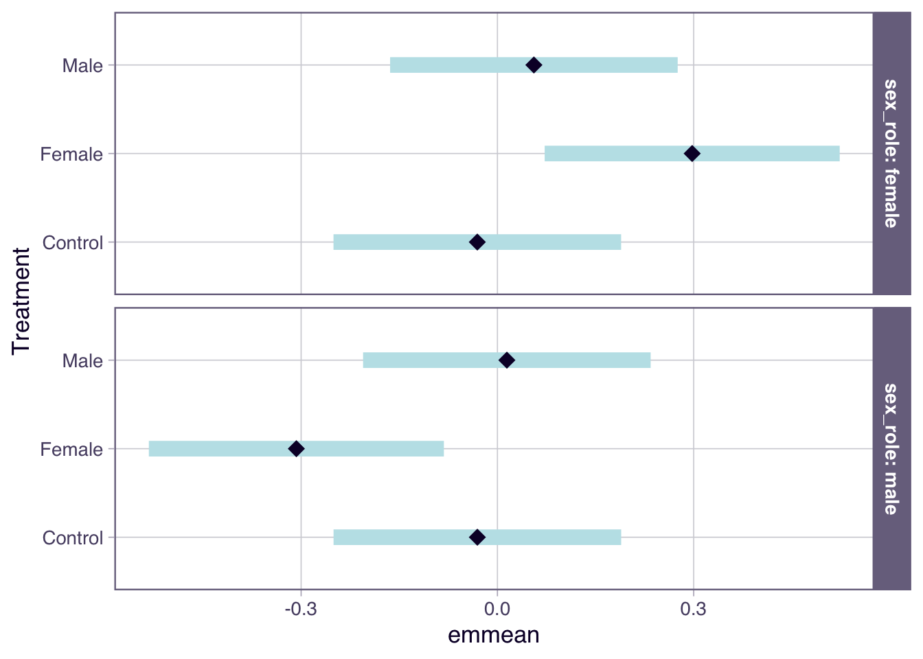
| Version | Author | Date |
|---|---|---|
| 7057ba1 | luekholman | 2026-02-09 |
cohens_d <- emmeans(modfitCS, ~ Treatment | sex_role) %>%
  pairs() %>% as_tibble() %>%
  filter(str_detect(contrast, "Control")) %>%
  select(trait = contrast, Estimate = estimate, SE)

cohens_d$trait <- c(
  "Female fitness (effect of feminising allele)",
  "Female fitness (effect of masculinising allele)",
  "Male fitness (effect of feminising allele)",
  "Male fitness (effect of masculinising allele)")

cohens_d$Estimate <- cohens_d$Estimate * c(-1, 1, 1, -1)

cohens_d$Lower_95_CI <- cohens_d$Estimate - cohens_d$SE * 1.96
cohens_d$Upper_95_CI <- cohens_d$Estimate + cohens_d$SE * 1.96

tibble(Study = "Nordén et al. (2020) Evolution 77, 1066-1076",
       Trait = cohens_d$trait,
       Generations = 14,
       Organism = "Macrostomum lignano",
       Interpretation = c(
         "The positive effect size means that worms carrying the feminising allele had higher fitness when breeding in the female sex role compared to worms carrying the control allele.",
         "A positive effect would mean that worms carrying the masculinising allele had lower fitness when breeding in the female sex role compared to worms carrying the control allele (actually, they had non-significantly higher fitness).",
         "A positive effect would mean that worms carrying the feminising allele had lower fitness when breeding in the male sex role compared to worms carrying the control allele (they did, but the difference is not significant).",
         "A positive effect would mean that worms carrying the masculinising allele had higher fitness when breeding in the male sex role compared to worms carrying the control allele (they did, but the difference is not significant)."
       ),
       Estimate = cohens_d$Estimate,
       Var = cohens_d$SE ^ 2,
       Lower_95_CI = cohens_d$Lower_95_CI,
       Upper_95_CI = cohens_d$Upper_95_CI) %>%
  write_csv("effect_sizes/norden2020.csv")
Middle-class neighbourhood experiments
This section covers publications that used a sex-specific middle class neighbourhood to relax selection on one sex. In general, I predict reduced fitness for the unselected sex, increased fitness in the other sex (due to the spread of sexually antagonistic alleles benefitting the selected sex), and phenotypic evolution towards the typical trait values for the selected sex (e.g. in Drosophila, chromosomes that had undergone male-limited evolution in should encode smaller body size and slower development time). The effect size signs selected reflect these expectations.
Radwan et al. (2004)
Radwan, J., Unrug, J., Snigórska, K., & Gawrońska, K. (2004). Effectiveness of sexual selection in preventing fitness deterioration in bulb mite populations under relaxed natural selection. Journal of Evolutionary Biology, 17(1), 94–99.
Radwan’s original data
The means and standard errors for each variable and treatment group were extracted from Table 1. Sample sizes for individual treatments are not given, so I divided the total sample size by 3 and rounded off to estimate them.
df <- tibble(
  Variable = rep(c("Viability",
                   "Female longevity",
                   "Female fecundity",
                   "Male fitness"),2),

  Treatment = c(rep("SS", 4), rep("C", 4)),

  mean = c(0.761, 23.74, 108.7, 0.543, 0.733, 25.35, 131.7, 0.596),
  SE   = c(0.102, 2.45, 4.47, 0.077, 0.066, 1.17, 9.51, 0.061),
  n = round(rep(c(161/3, 136/3, 139/3, 100/3), 2))
)

kable(df) %>%
kable_styling(full_width = F)| Variable | Treatment | mean | SE | n |
|---|---|---|---|---|
| Viability | SS | 0.761 | 0.102 | 54 |
| Female longevity | SS | 23.740 | 2.450 | 45 |
| Female fecundity | SS | 108.700 | 4.470 | 46 |
| Male fitness | SS | 0.543 | 0.077 | 33 |
| Viability | C | 0.733 | 0.066 | 54 |
| Female longevity | C | 25.350 | 1.170 | 45 |
| Female fecundity | C | 131.700 | 9.510 | 46 |
| Male fitness | C | 0.596 | 0.061 | 33 |
Viability
mes(m.2 = df$mean[df$Treatment=="SS" & df$Variable == "Viability"],
    m.1 = df$mean[df$Treatment=="C" & df$Variable == "Viability"],
    sd.2 = df$SE[df$Treatment=="SS" & df$Variable == "Viability"] *
      sqrt(df$n[df$Treatment=="SS" & df$Variable == "Viability"]),
    sd.1 = df$SE[df$Treatment=="C" & df$Variable == "Viability"] *
      sqrt(df$n[df$Treatment=="C" & df$Variable == "Viability"]),
    n.2 = df$n[df$Treatment=="SS" & df$Variable == "Viability"],
    n.1 = df$n[df$Treatment=="C" & df$Variable == "Viability"], verbose=F) %>%
  parse_es(study = "Radwan et al. (2004) J. Evol. Biol. 17, 94–99.",
           generations = 11,
           organism = "Rhizoglyphus robini",
           trait = "Viability",
           interpretation = "A positive effect size would indicate lower viability in populations that experienced relaxed selection on females relative to those experiencing selection on both sexes (the difference is non-significant and in the opposite direction)."
          ) %>%
  write_csv("effect_sizes/radwan2004_1.csv")
Female longevity
mes(m.2 = df$mean[df$Treatment=="SS" & df$Variable == "Female longevity"],
    m.1 = df$mean[df$Treatment=="C" & df$Variable == "Female longevity"],
    sd.2 = df$SE[df$Treatment=="SS" & df$Variable == "Female longevity"] *
      sqrt(df$n[df$Treatment=="SS" & df$Variable == "Female longevity"]),
    sd.1 = df$SE[df$Treatment=="C" & df$Variable == "Female longevity"] *
      sqrt(df$n[df$Treatment=="C" & df$Variable == "Female longevity"]),
    n.2 = df$n[df$Treatment=="SS" & df$Variable == "Female longevity"],
    n.1 = df$n[df$Treatment=="C" & df$Variable == "Female longevity"], verbose=F) %>%
  parse_es(study = "Radwan et al. (2004) J. Evol. Biol. 17, 94–99.",
           generations = 11,
           organism = "Rhizoglyphus robini",
           trait = "Female longevity",
           interpretation = "A positive effect size would indicate reduced female longevity in populations that experienced relaxed selection on females relative to those experiencing selection on both sexes (the difference is non-significant and in the predicted direction).") %>%
  write_csv("effect_sizes/radwan2004_2.csv")
Female fecundity
mes(m.2 = df$mean[df$Treatment=="SS" & df$Variable == "Female fecundity"],
    m.1 = df$mean[df$Treatment=="C" & df$Variable == "Female fecundity"],
    sd.2 = df$SE[df$Treatment=="SS" & df$Variable == "Female fecundity"] *
      sqrt(df$n[df$Treatment=="SS" & df$Variable == "Female fecundity"]),
    sd.1 = df$SE[df$Treatment=="C" & df$Variable == "Female fecundity"] *
      sqrt(df$n[df$Treatment=="C" & df$Variable == "Female fecundity"]),
    n.2 = df$n[df$Treatment=="SS" & df$Variable == "Female fecundity"],
    n.1 = df$n[df$Treatment=="C" & df$Variable == "Female fecundity"], verbose=F) %>%
  parse_es(study = "Radwan et al. (2004) J. Evol. Biol. 17, 94–99.",
           generations = 11,
           organism = "Rhizoglyphus robini",
           trait = "Female fecundity",
           interpretation = "The positive effect size indicates reduced fecundity in populations that experienced relaxed selection on females relative to those experiencing selection on both sexes.") %>%
  write_csv("effect_sizes/radwan2004_3.csv")
Male fitness
mes(m.1 = df$mean[df$Treatment=="SS" & df$Variable == "Male fitness"],
    m.2 = df$mean[df$Treatment=="C" & df$Variable == "Male fitness"],
    sd.1 = df$SE[df$Treatment=="SS" & df$Variable == "Male fitness"] *
      sqrt(df$n[df$Treatment=="SS" & df$Variable == "Male fitness"]),
    sd.2 = df$SE[df$Treatment=="C" & df$Variable == "Male fitness"] *
      sqrt(df$n[df$Treatment=="C" & df$Variable == "Male fitness"]),
    n.1 = df$n[df$Treatment=="SS" & df$Variable == "Male fitness"],
    n.2 = df$n[df$Treatment=="C" & df$Variable == "Male fitness"], verbose=F) %>%
  parse_es(study = "Radwan et al. (2004) J. Evol. Biol. 17, 94–99.",
           generations = 11,
           organism = "Rhizoglyphus robini",
           trait = "Male fitness",
           interpretation = "A positive effect size would indicate increased fitness in populations that experienced relaxed selection on females relative to those experiencing selection on both sexes (the difference is non-significant and in the opposite direction).") %>%
  write_csv("effect_sizes/radwan2004_4.csv")
Morrow et al. (2008)
Morrow, E. H., Stewart, A. D., & Rice, W. R. (2008). Assessing the extent of genome-wide intralocus sexual conflict via experimentally enforced gender-limited selection. Journal of Evolutionary Biology, 21(4), 1046–1054.
Morrow et al.’s original data
df <- tibble(treatment = c("selected sex", "non-selected sex","selected sex", "non-selected sex"),
       trait = c("male fitness", "male fitness", "female fitness", "female fitness"),
       mean = c(9.761182759612618, 8.5105834691725, 38.60211669355156, 33.71168902702915),
       SE = c(10.07670917633522 - 9.761182759612618,
              8.812266276728353 - 8.5105834691725,
              38.99686561487718 - 38.60211669355156,
              33.985783792999435 - 33.71168902702915),
       N = c(60, 60, 60, 60))

kable(df) %>%
kable_styling(full_width = F)| treatment | trait | mean | SE | N |
|---|---|---|---|---|
| selected sex | male fitness | 9.761183 | 0.3155264 | 60 |
| non-selected sex | male fitness | 8.510583 | 0.3016828 | 60 |
| selected sex | female fitness | 38.602117 | 0.3947489 | 60 |
| non-selected sex | female fitness | 33.711689 | 0.2740948 | 60 |
Male fitness effect size
mes(m.1 = df$mean[df$trait == "male fitness" & df$treatment == "selected sex"],
    m.2 = df$mean[df$trait == "male fitness" & df$treatment == "non-selected sex"],
    sd.1 = df$SE[df$trait == "male fitness" & df$treatment == "selected sex"] * sqrt(60),
    sd.2 = df$SE[df$trait == "male fitness" & df$treatment == "non-selected sex"] * sqrt(60),
    n.1 = 60, n.2 = 60, verbose = F) %>%
  parse_es(study = "Morrow et al. (2008) J. Evol. Biol. 21, 1046–1054",
           trait = "Male fitness",
           generations = 26,
           organism = "Drosophila melanogaster",
           interpretation = "The positive effect sie indicates that male fitness was higher in lines where selection was relaxed on females compared to lines where selection was relaxed on males.") %>%
  write_csv("effect_sizes/morrow2008_1.csv")
Female fitness effect size
mes(m.1 = df$mean[df$trait == "female fitness" & df$treatment == "selected sex"],
    m.2 = df$mean[df$trait == "female fitness" & df$treatment == "non-selected sex"],
    sd.1 = df$SE[df$trait == "female fitness" & df$treatment == "selected sex"] * sqrt(60),
    sd.2 = df$SE[df$trait == "female fitness" & df$treatment == "non-selected sex"] * sqrt(60),
    n.1 = 60, n.2 = 60, verbose = F) %>%
  parse_es(study = "Morrow et al. (2008) J. Evol. Biol. 21, 1046–1054",
           trait = "Female fitness",
           generations = 26,
           organism = "Drosophila melanogaster",
           interpretation = "The positive effect sie indicates that female fitness was higher in lines where selection was relaxed on males compared to lines where selection was relaxed on females.") %>%
  write_csv("effect_sizes/morrow2008_2.csv")
Martinossi-Allibert et al. (2019)
Martinossi-Allibert, I., Thilliez, E., Arnqvist, G., & Berger, D. (2019). Sexual selection, environmental robustness, and evolutionary demography of maladapted populations: A test using experimental evolution in seed beetles. Evolutionary Applications, 12(7), 1371–1384.
I obtained the raw data from Dryad, ran a GLMM with formula
LRS ~ treatment*sex*environment + (1 | line), and used
emmeans to get the treatment effect on LRS for each sex (averaging over
levels of environment). I scaled LRS first, so the treatment effects are
equal to Cohen’s d.
I focus on the difference between the female-specific middle class neighbourhood treatment and the monogamy treatment (the latter has natural selection on both sexes but not sexual selection, while the former has natural and sexual selection on males and relaxed selection on females). The authors re-branded the female-MCN treatment as a “sexual selection only” (S treatment) in a later paper (Baur and Berger 2020, below), though it would seem to allow for natural selection on males as well.
Female fitness
Martinossi_Allibert <- read_excel("input_data/MartinossiAllibert_dryad_data.xlsx", sheet = "LRS") %>%
  select(treatment = Evolution_tSeatment_type,
         replicate = Evolution_treatment_replicate,
         line = Evolution_treatment_unique,
         environment = Assay_environment,
         sex = Sex,
         LRS = Rel_to_pol29_persex) %>%
  mutate(treatment = replace(treatment, treatment == "F", "Monogamy"),
         treatment = replace(treatment, treatment == "M", "Malelimited"),
         treatment = replace(treatment, treatment == "S", "Polygamy"),
         LRS = as.numeric(scale(LRS)))
New names:
• `` -> `...17`
• `` -> `...18`
• `` -> `...19`
• `` -> `...20`es <- (emmeans(lmer(LRS~ treatment*sex*environment + (1 | line),
data = Martinossi_Allibert), specs = c("treatment", "sex")) %>%
pairs() %>%
as_tibble() %>%
filter(str_detect(contrast, "Malelimited") & str_detect(contrast, "Monogamy")))[c(1,4), ] Note: D.f. calculations have been disabled because the number of observations exceeds 3000.
To enable adjustments, add the argument 'pbkrtest.limit = 3672' (or larger)
[or, globally, 'set emm_options(pbkrtest.limit = 3672)' or larger];
but be warned that this may result in large computation time and memory use.
Note: D.f. calculations have been disabled because the number of observations exceeds 3000.
To enable adjustments, add the argument 'lmerTest.limit = 3672' (or larger)
[or, globally, 'set emm_options(lmerTest.limit = 3672)' or larger];
but be warned that this may result in large computation time and memory use.
NOTE: Results may be misleading due to involvement in interactionses$estimate[1] <- es$estimate[1] * -1 # flip effect size sign for females
es <- es %>%
mutate(Lower_95_CI = estimate - SE*1.96,
Upper_95_CI = estimate + SE*1.96)
tibble(
Study = "Martinossi-Allibert et al. (2019) Evol. Applic., 12, 1371–1384",
Trait = "Female fitness",
Generations = 16,
Organism = "Callosobruchus maculatus",
Interpretation = "A positive effect would indicate that the relaxation of selection on females reduced female fitness, relative to the monogamy treatment which removed sexual selection yet maintained natural selection on both sexes (there is non-significant difference in the opposite direction).",
Estimate = es$estimate[1],
Var = es$SE[1] ^ 2,
Lower_95_CI = es$Lower_95_CI[1],
Upper_95_CI = es$Upper_95_CI[1]) %>%
write_csv("effect_sizes/martinossiAllibert2019_1.csv")Male fitness
tibble(
  Study = "Martinossi-Allibert et al. (2019) Evol. Applic., 12, 1371–1384",
  Trait = "Male fitness",
  Generations = 16,
  Organism = "Callosobruchus maculatus",
  Interpretation = "The positive effect indicates that the relaxation of selection on females increased male fitness, relative to the monogamy treatment which removed sexual selection yet maintained natural selection on both sexes.",
  Estimate = es$estimate[2],
  Var = es$SE[2] ^ 2,
  Lower_95_CI = es$Lower_95_CI[2],
  Upper_95_CI = es$Upper_95_CI[2]) %>%
  write_csv("effect_sizes/martinossiAllibert2019_2.csv")
Baur and Berger (2020)
Baur, J., & Berger, D. (2020). Experimental evidence for effects of sexual selection on condition-dependent mutation rates. Nature Ecology & Evolution, 4(5), 737–744.
This study is mentioned in the paper, but I elected not to include it in the meta-analysis as it’s unclear what the predictions should be under our hypothesis that there is intralocus sexual conflict. The study compares an ‘N’ treatment that was essentially enforced random monogamy with an ‘S’ treatment that relaxed selection on females and allowed sexual (and natural) selection on males. The S populations experience a lower fitness decline after irradiation, suggesting they are more resistant to mutation. But it’s unclear whether the fixation of male-benefit female-detriment alleles in the S treatment should necessarily improve or reduce mutation resistance.
sessionInfo()R version 4.5.2 (2025-10-31)
Platform: aarch64-apple-darwin20
Running under: macOS Tahoe 26.2
Matrix products: default
BLAS: /System/Library/Frameworks/Accelerate.framework/Versions/A/Frameworks/vecLib.framework/Versions/A/libBLAS.dylib
LAPACK: /Library/Frameworks/R.framework/Versions/4.5-arm64/Resources/lib/libRlapack.dylib; LAPACK version 3.12.1
locale:
[1] en_US.UTF-8/en_US.UTF-8/en_US.UTF-8/C/en_US.UTF-8/en_US.UTF-8
time zone: Europe/London
tzcode source: internal
attached base packages:
[1] stats graphics grDevices utils datasets methods base
other attached packages:
[1] compute.es_0.2-6 kableExtra_1.4.0 survival_3.8-3 emmeans_2.0.1
[5] lmerTest_3.2-0 car_3.1-5 carData_3.0-6 lme4_1.1-38
[9] Matrix_1.7-4 readxl_1.4.5 lubridate_1.9.4 forcats_1.0.1
[13] stringr_1.6.0 dplyr_1.2.0 purrr_1.2.1 readr_2.1.6
[17] tidyr_1.3.2 tibble_3.3.1 ggplot2_4.0.2 tidyverse_2.0.0
[21] workflowr_1.7.2
loaded via a namespace (and not attached):
[1] tidyselect_1.2.1 viridisLite_0.4.2 farver_2.1.2
[4] S7_0.2.1 fastmap_1.2.0 promises_1.5.0
[7] digest_0.6.39 timechange_0.4.0 estimability_1.5.1
[10] lifecycle_1.0.5 processx_3.8.6 magrittr_2.0.4
[13] compiler_4.5.2 rlang_1.1.7 sass_0.4.10
[16] tools_4.5.2 yaml_2.3.12 knitr_1.51
[19] labeling_0.4.3 bit_4.6.0 xml2_1.5.2
[22] RColorBrewer_1.1-3 abind_1.4-8 withr_3.0.2
[25] numDeriv_2016.8-1.1 grid_4.5.2 git2r_0.36.2
[28] scales_1.4.0 MASS_7.3-65 cli_3.6.5
[31] mvtnorm_1.3-3 crayon_1.5.3 rmarkdown_2.30
[34] reformulas_0.4.4 generics_0.1.4 otel_0.2.0
[37] rstudioapi_0.18.0 httr_1.4.7 tzdb_0.5.0
[40] minqa_1.2.8 cachem_1.1.0 splines_4.5.2
[43] parallel_4.5.2 cellranger_1.1.0 vctrs_0.7.1
[46] boot_1.3-32 jsonlite_2.0.0 callr_3.7.6
[49] hms_1.1.4 pbkrtest_0.5.5 bit64_4.6.0-1
[52] Formula_1.2-5 systemfonts_1.3.1 jquerylib_0.1.4
[55] glue_1.8.0 nloptr_2.2.1 ps_1.9.1
[58] stringi_1.8.7 gtable_0.3.6 later_1.4.5
[61] pillar_1.11.1 htmltools_0.5.9 R6_2.6.1
[64] textshaping_1.0.4 Rdpack_2.6.5 rprojroot_2.1.1
[67] vroom_1.7.0 evaluate_1.0.5 lattice_0.22-7
[70] backports_1.5.0 rbibutils_2.4.1 broom_1.0.12
[73] httpuv_1.6.16 bslib_0.10.0 Rcpp_1.1.1
[76] svglite_2.2.2 coda_0.19-4.1 nlme_3.1-168
[79] whisker_0.4.1 xfun_0.56 fs_1.6.6
[82] getPass_0.2-4 pkgconfig_2.0.3