Last updated: 2021-03-12

Checks: 7 0

Knit directory: exp_evol_respiration/

This reproducible R Markdown analysis was created with workflowr (version 1.6.2). The Checks tab describes the reproducibility checks that were applied when the results were created. The Past versions tab lists the development history.

R Markdown file: up-to-date

Great! Since the R Markdown file has been committed to the Git repository, you know the exact version of the code that produced these results.

Environment: empty

Great job! The global environment was empty. Objects defined in the global environment can affect the analysis in your R Markdown file in unknown ways. For reproduciblity it’s best to always run the code in an empty environment.

Seed: set.seed(20190703)

The command set.seed(20190703) was run prior to running the code in the R Markdown file. Setting a seed ensures that any results that rely on randomness, e.g. subsampling or permutations, are reproducible.

Session information: recorded

Great job! Recording the operating system, R version, and package versions is critical for reproducibility.

Cache: none

Nice! There were no cached chunks for this analysis, so you can be confident that you successfully produced the results during this run.

File paths: relative

Great job! Using relative paths to the files within your workflowr project makes it easier to run your code on other machines.

Repository version: f7b49ff

Great! You are using Git for version control. Tracking code development and connecting the code version to the results is critical for reproducibility.

The results in this page were generated with repository version f7b49ff. See the Past versions tab to see a history of the changes made to the R Markdown and HTML files.

Note that you need to be careful to ensure that all relevant files for the analysis have been committed to Git prior to generating the results (you can use wflow_publish or wflow_git_commit). workflowr only checks the R Markdown file, but you know if there are other scripts or data files that it depends on. Below is the status of the Git repository when the results were generated:


Ignored files:
    Ignored:    .DS_Store
    Ignored:    .Rhistory
    Ignored:    .Rproj.user/
    Ignored:    figures/.DS_Store
    Ignored:    output/.DS_Store

Untracked files:
    Untracked:  data/1.eclosion_wide.csv
    Untracked:  figures/desiccation.pdf
    Untracked:  figures/eclosion.pdf
    Untracked:  figures/metaboliteDAG.pdf
    Untracked:  figures/metabolite_plotCONTROLLED.pdf
    Untracked:  figures/metabolites_supp.pdf
    Untracked:  figures/respirationDAG.pdf
    Untracked:  figures/respiration_figure_noRQ.pdf
    Untracked:  figures/starvation.pdf
    Untracked:  output/stress_medians.csv

Unstaged changes:
    Modified:   figures/metabolite_interaction_plot.pdf
    Modified:   figures/metabolite_pairs_plot.pdf
    Modified:   figures/metabolite_plot.pdf
    Modified:   figures/respiration_figure.pdf
    Modified:   figures/respiration_pairs_plot.pdf
    Modified:   output/cox_brms.rds
    Deleted:    output/coxmod.rds
    Deleted:    output/coxmod_dropINT.rds
    Deleted:    output/coxmod_dropSEX.rds
    Deleted:    output/coxmod_dropTRT.rds

Note that any generated files, e.g. HTML, png, CSS, etc., are not included in this status report because it is ok for generated content to have uncommitted changes.

These are the previous versions of the repository in which changes were made to the R Markdown (analysis/juvenile_development.Rmd) and HTML (docs/juvenile_development.html) files. If you’ve configured a remote Git repository (see ?wflow_git_remote), click on the hyperlinks in the table below to view the files as they were in that past version.

File	Version	Author	Date	Message
Rmd	f7b49ff	MartinGarlovsky	2021-03-12	wflow_publish(c(“analysis/juvenile_development.Rmd”, “analysis/resistance.Rmd”,
html	ffb09dd	MartinGarlovsky	2021-02-08	Build site.
Rmd	1b92046	MartinGarlovsky	2021-02-08	wflow_publish(c(“analysis/juvenile_development.Rmd”, “analysis/resistance.Rmd”,
html	ae3c04b	MartinGarlovsky	2021-02-06	Build site.
Rmd	25528a3	MartinGarlovsky	2021-02-06	wflow_publish(“analysis/juvenile_development.Rmd”)
html	709456c	Martin Garlovsky	2021-01-18	Build site.
Rmd	c2d846f	Martin Garlovsky	2021-01-18	wflow_publish(c(“analysis/juvenile_development.Rmd”, “analysis/resistance.Rmd”,
html	d19a7e6	lukeholman	2020-12-18	Build site.
Rmd	a0c557c	lukeholman	2020-12-18	new title
html	41d232f	lukeholman	2020-12-18	Build site.
html	6861115	lukeholman	2020-12-18	Build site.
html	0d5bcc9	lukeholman	2020-12-18	Build site.
html	989e86f	lukeholman	2020-12-18	Build site.
Rmd	5a81a83	lukeholman	2020-12-18	new menu
Rmd	96d1188	Martin Garlovsky	2020-12-13	MDG commit
html	96d1188	Martin Garlovsky	2020-12-13	MDG commit
Rmd	7d4b609	Martin Garlovsky	2020-12-05	MDG commit
html	7d4b609	Martin Garlovsky	2020-12-05	MDG commit
html	df61dde	Martin Garlovsky	2020-12-04	MDG commit
Rmd	0714753	Martin Garlovsky	2020-12-04	workflowr::wflow_git_commit(all = T)
Rmd	3fdbcb2	lukeholman	2020-11-30	Tweaks Nov 2020

Load packages

library(tidyverse)
library(ggridges)

library(coxme)
library(brms)
library(tidybayes)

library(kableExtra)
library(knitrhooks) # install with devtools::install_github("nathaneastwood/knitrhooks")
library(showtext)

output_max_height() # a knitrhook option

options(stringsAsFactors = FALSE)

# set up nice font for figure
nice_font <- "Lora"
font_add_google(name = nice_font, family = nice_font, regular.wt = 400, bold.wt = 700)
showtext_auto()

Load data

# load eclosion data
eclosion_wide <- read.csv("data/1.eclosion_wide.csv")

# convert data to 'long' format
eclosion_long <- reshape2::melt(eclosion_wide, id.vars = "DAY")

# add ID columns
eclosion_long$YEAR <- factor("2015")
eclosion_long$variable <- paste(eclosion_long$variable, eclosion_long$YEAR, sep = "_")
eclosion_long$ID <- gsub(pattern = "_m|f_", replacement = "", x = eclosion_long$variable)

# calculate days to eclosion starting from seeding day
eclosion_long <- eclosion_long %>% 
  separate(variable, c("LINE", "SEED", "VIAL", "SEX", "YEAR")) %>% 
  mutate(SEED_DAY = case_when(SEED == 'A' ~ "2015-7-20", 
                              SEED == 'B' ~ "2015-7-21",
                              SEED == 'C' ~ "2015-7-22"),
         START_DAY = case_when(SEED == 'A' ~ "2015-8-01", 
                               SEED == 'B' ~ "2015-8-02",
                               SEED == "C" & 
                                 LINE == "M1"| LINE == "M2"| LINE == "M3"| LINE == "M4" ~ "2015-8-03",
                               TRUE ~ "2015-8-04"),
         DAY_ZERO = as.numeric(as.Date(START_DAY) - as.Date(SEED_DAY)),
         DAY = DAY + DAY_ZERO)


# remove rows where no flies eclosed
eclosion_long <- subset(eclosion_long, value>0)

# add event 
eclosion_long$EVENT <- 1

# calulate number not eclosed for each vial (out of 100)
uneclosed <- as.data.frame(eclosion_long %>% 
                             group_by(ID, LINE, SEED, VIAL) %>% 
                             summarise(SEX = "fm",
                                       DAY = 21,
                                       eclosing = 100 - sum(value),
                                       EVENT = 0,
                                       YEAR = "2015"))


# calculate proportion eclosed of each sex to give weights to uneclosed
p <- eclosion_long %>% group_by(SEX) %>% summarise(S = sum(value))
prop.male <- p$S[2]/(p$S[2]+p$S[1])
prop.female <- p$S[1]/(p$S[2]+p$S[1])

# assign sex to uneclosed in each vial based on those that have eclosed... i.e. slighly more females already eclosed
uneclosed.male <- mutate(uneclosed, 
                            SEX = "m", eclosing = round(uneclosed$eclosing*prop.female))

uneclosed.female <- mutate(uneclosed, 
                              SEX = "f", eclosing = round(uneclosed$eclosing*prop.male))

colnames(eclosion_long)[7] <- "eclosing"

# reorder columns
eclosion_long <- eclosion_long %>% select(ID, DAY, SEX, LINE, SEED, VIAL, YEAR, eclosing, EVENT)

# bind eclosed data to calculated uneclosed
eclosion_long <- rbind(eclosion_long, uneclosed.male, uneclosed.female)
eclosion_long <- eclosion_long[order(eclosion_long$ID, eclosion_long$SEX), ]

# add treatment variable 
eclosion_long$TRT <- factor(substr(eclosion_long$ID, 1, 1))

# remove vials seeded with more than 100 larvae
#unique(eclosion.dat[which(eclosion.dat$eclosing < 0), "ID"]) # 4 vials overseeded
eclosion.dat.trim <- eclosion_long %>% 
  filter(ID %in% eclosion_long[which(eclosion_long$eclosing < 0), "ID"] == FALSE)

# expand data frame so each row is a single fly
ecl.dat <- reshape::untable(eclosion.dat.trim[ ,c(1:7, 9, 10)], 
                           num = eclosion.dat.trim[, 8])

# load wing length data
wing_length <- read.csv("data/1.wing_length.csv") %>% 
  filter(Side == 'L') %>% 
  # scale wing vein length to make effect size comparisons with other data sets?
  mutate(Length = as.numeric(scale(Length)))

# add replicate
wing_length$LINE <- paste0(wing_length$Treatment, substr(wing_length$Rep, 2, 2))

Inspecting the raw data

ecl.dat %>% 
  filter(EVENT == 1) %>% 
  select(TRT, SEX, DAY) %>% 
  mutate(TRT_SEX = paste0(TRT, SEX),
         SEX = factor(ifelse(SEX == "m", "Males", "Females"))) %>% 
  ggplot(aes(x = DAY, y = SEX, fill = TRT_SEX)) +
  geom_boxplot() +
  scale_fill_manual(values = c("pink", "skyblue", "red", "blue"), name = "",
                    labels = c('Monogamy Females', 'Monogamy Males',
                               'Polandry Females', 'Polandry Males')) +
  labs(x = 'Eclosion time (days)', y = 'Sex') +
  theme_bw() +
  NULL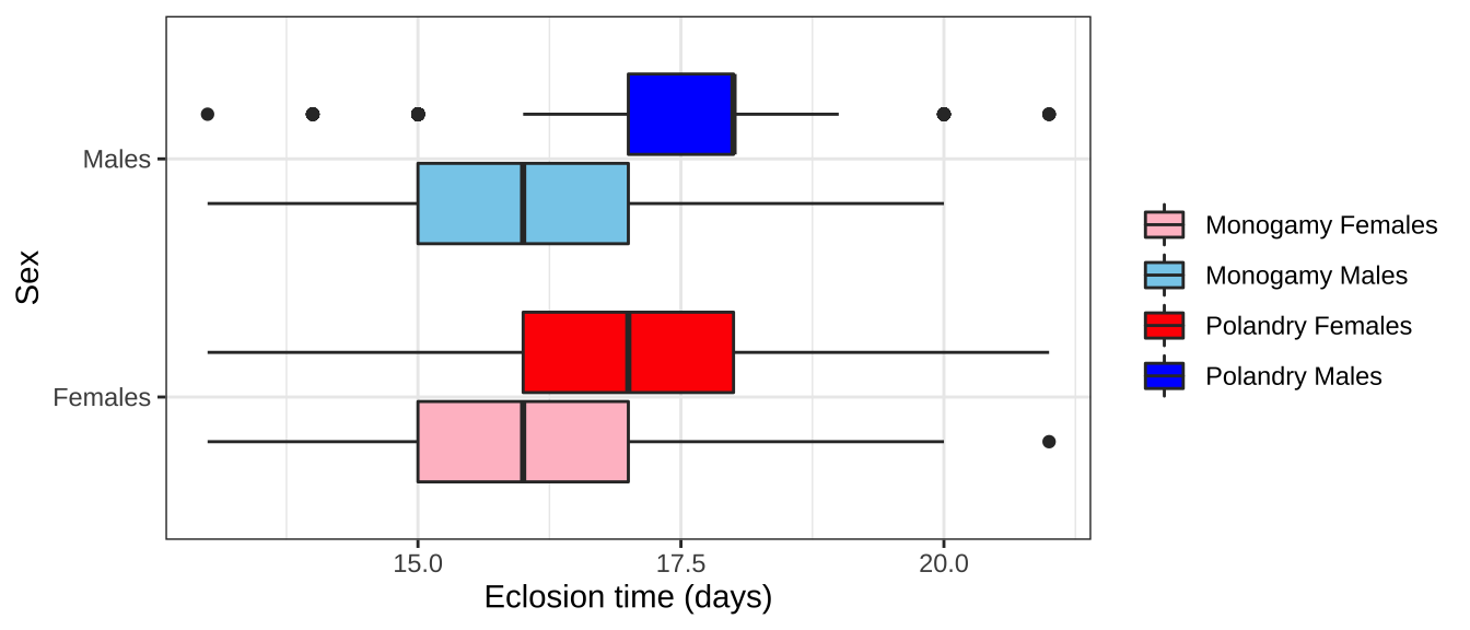

Version	Author	Date
ae3c04b	MartinGarlovsky	2021-02-06
709456c	Martin Garlovsky	2021-01-18
989e86f	lukeholman	2020-12-18
96d1188	Martin Garlovsky	2020-12-13
df61dde	Martin Garlovsky	2020-12-04

Survival analysis

We modelled juvenile development time using survival analysis. We measured the time in days from 1st instar larvae until eclosion (EVENT = 1) upon which flies were stored in ethanol before counting. Of the initially seeded 100 flies per vial, the remaining flies not emerging after two consecutive days of no observed eclosions were right censored (EVENT = 0) on the last observation day. In total 14400 larvae were seeded (100 larvae x 2 Treatment x 4 LINE per Treatment x 6 VIAL per LINE x 3 SEED days). For P1 only three vials were seeded on day B so we seeded 3 additional vials on day C. Four vials were seeded with too many larvae and excluded from analysis. In total 10448 flies eclosed during the observation period leaving 3552 individuals to be right censored on day 9.

Censoring

Censored flies were assigned sex based on the observed sex ratio of eclosees assuming an equal (50:50) sex ratio of larvae seeded to each vial at the beginning of the experiment. We calculate the number of number of males and females that did eclose and subsequently assign sex to the remaining (uneclosed) individuals of unknown sex based on the proportion of individuals of each sex that did emerge. For example, if 70 flies were counted eclosing from a vial with 40 females and 30 males, we then designate the remaining 30 flies as 10 females and 20 males and so on so that each vial ends with 50 females and 50 males some of which are right censored (EVENT = 0).

Kaplan-Meier survival curve

First we plot Kaplan-Meier survival curves without considering our full experimental design.

survminer::ggsurvplot(survfit(Surv(DAY, EVENT) ~ TRT + SEX, data = ecl.dat),
                      conf.int = TRUE,
                      risk.table = FALSE,
                      linetype = "SEX",
                      palette = c("pink", "skyblue", "red", "blue"),
                      fun = "event",
                      xlim = c(12, 21),
                      xlab = "Days",
                      legend = 'right',
                      legend.title = "",
                      legend.labs = c("M \u2640","M \u2642",'E \u2640','E \u2642'),
                      break.time.by = 2,
                      ggtheme = theme_bw())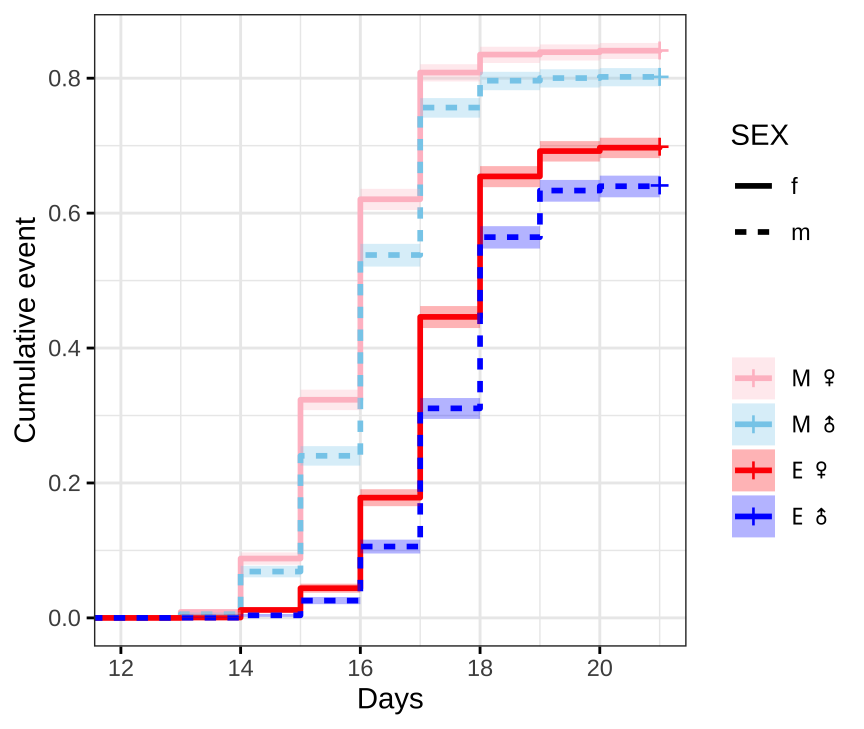

Version	Author	Date
ae3c04b	MartinGarlovsky	2021-02-06
709456c	Martin Garlovsky	2021-01-18
989e86f	lukeholman	2020-12-18
96d1188	Martin Garlovsky	2020-12-13
7d4b609	Martin Garlovsky	2020-12-05
df61dde	Martin Garlovsky	2020-12-04

#ggsave(filename = 'figures/eclosion.pdf', width = 5.5, height = 5, dpi = 600, useDingbats = FALSE)

Figure X: Kaplan-Meier curve for eclosion time (in days) for flies in each treatment and sex. +’s indicate censored individuals (n = 3552).

Median eclosion times

summary(survfit(Surv(DAY, EVENT) ~ TRT + SEX, data = ecl.dat))$table %>% 
  as_tibble() %>% 
  mutate(Treatment = c('M', 'M', 'E', 'E'),
         Sex = c('Female', 'Male', 'Female', 'Male')) %>% 
  mutate(`Median (± 95% CI)` = paste0(median, ' (', `0.95LCL`, '-', `0.95UCL`, ')')) %>% 
  dplyr::select(Treatment, Sex, N = records, `N events` = events, `Median (± 95% CI)`) %>%
  kable() %>% 
  kable_styling(full_width = FALSE)

Treatment	Sex	N	N events	Median (± 95% CI)
M	Female	3637	3059	16 (16-16)
M	Male	3363	2697	16 (16-16)
E	Female	3568	2492	18 (18-18)
E	Male	3432	2200	18 (18-18)

Check proportional hazards assumption

Next we need to check that the proportional hazards assumption is not violated before fitting the model, where crossing hazards (lines) indicate violation of the proportional hazards assumption.

survminer::ggsurvplot(survfit(Surv(DAY, EVENT) ~ TRT + SEX, data = ecl.dat),
                      conf.int = TRUE,
                      risk.table = FALSE,
                      linetype = "SEX",
                      palette = c("pink", "skyblue", "red", "blue"),
                      fun = "cloglog",
                      xlim = c(13, 21),
                      legend = 'right',
                      legend.title = "",
                      legend.labs = c("M \u2640","M \u2642",'E \u2640','E \u2642'),
                      break.time.by = 2,
                      ggtheme = theme_bw())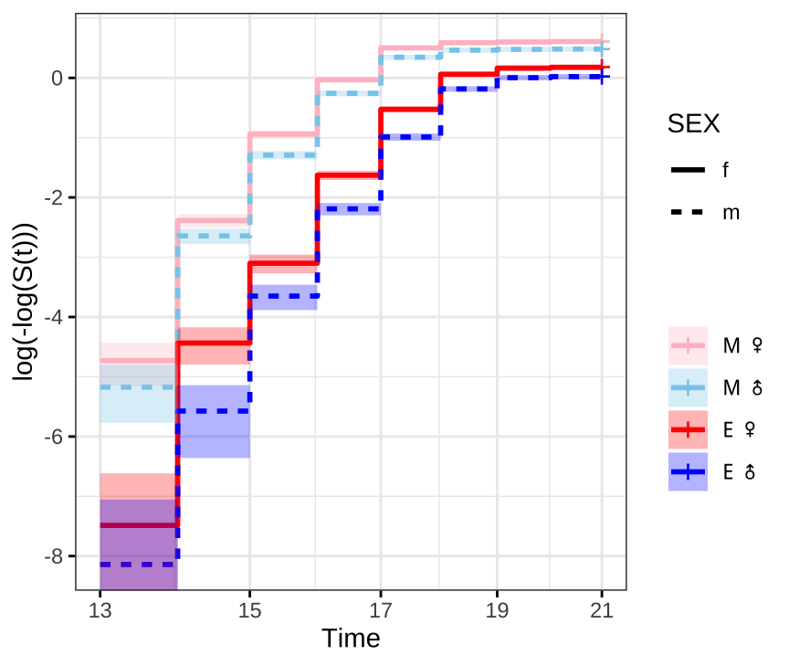

Version	Author	Date
709456c	Martin Garlovsky	2021-01-18
989e86f	lukeholman	2020-12-18
96d1188	Martin Garlovsky	2020-12-13
7d4b609	Martin Garlovsky	2020-12-05
df61dde	Martin Garlovsky	2020-12-04

Figure X: ln(-ln(survival))

Fit the model in `brms`

We fit a Cox Proportional hazards model in brms using family = cox(), with time (days) to event (eclosion) as the response and sexual selection treatment (TRT; Monogamy or Elevated polyandry), SEX (female or male) and their interaction as predictors with Seed day as a covariate. See here for a helpful explanation on fitting survival models in brms. We also include replicate treatment as a random intercept term for each of the 8 lines and a random slope term to allow the effect of selection treatment to vary across replicate lines. We also include vial ID as a random intercept term as individuals emerging from the same vial may show a correlated response.

Define priors

We set conservative normal priors on the fixed effects (mean = 0, sd = 1) and half Cauchy priors on the random effects - LINE and vial ID - (mean = 0, scale = 0.1). All other priors were left at the default in brms.

Run the model

The model is run over 4 chains with 5000 iterations each (with the first 2500 discarded as burn-in), for a total of 2500*4 = 10,000 posterior samples. Note that some of the brms functionality is not currently available for models using the cox family (e.g. posterior predictive checks).

if(!file.exists("output/cox_brms.rds")){
  
  cox_brm <- brm(DAY | cens(1 - EVENT) ~ TRT * SEX + SEED + (TRT|LINE) + (1|ID),
               iter = 5000, chains = 4, cores = 4,
               prior = c(set_prior("normal(0,1)", class = "b"),
                         set_prior("cauchy(0,0.1)", class = "sd")),
               control = list(max_treedepth = 20,
                              adapt_delta = 0.999),
               data = ecl.dat, family = cox())
  
  saveRDS(cox_brm, "output/cox_brms.rds")
} else {
  cox_brm <- readRDS('output/cox_brms.rds')
}

Table of model parameter estimates - eclosion time

Formatted table

This tables shows the fixed effects estimates on eclosion time. The p column shows 1 - minus the “probability of direction”, i.e. the posterior probability that the reported sign of the estimate is correct given the data and the prior; subtracting this value from one gives a Bayesian equivalent of a one-sided p-value. Click the next tab to see a complete summary of the model and its output.

hyp_test <- bind_rows(
  hypothesis(cox_brm, 'TRTP = 0')$hypothesis,
  hypothesis(cox_brm, 'SEXm = 0')$hypothesis,
  hypothesis(cox_brm, 'TRTP:SEXm = 0')$hypothesis,
  hypothesis(cox_brm, 'SEEDB = 0')$hypothesis,
  hypothesis(cox_brm, 'SEEDC = 0')$hypothesis
) %>% 
  mutate(Parameter = c('Treatment (E)', 'Sex (M)', 'Treatment (E) x Sex (M)', 'Seed (B)', 'Seed (C)'),
         across(2:5, round, 3)) %>% 
  relocate(Parameter, Estimate, Est.Error, CI.Lower, CI.Upper, Star)

pvals <- bayestestR::p_direction(cox_brm) %>% 
  as.data.frame() %>%
  mutate(vars = map_chr(str_split(Parameter, "_"), ~ .x[2]),
         p_val = 1 - pd, 
         star = ifelse(p_val < 0.05, "\\*", "")) %>%
  select(vars, p_val, star)

hyp_test %>% 
  mutate(vars = c('TRTP', 'SEXm', 'TRTP.SEXm', 'SEEDB', 'SEEDC')) %>% 
  left_join(pvals %>% filter(vars != 'Intercept'), 
            by = c("vars")) %>% 
  select(Parameter, Estimate, Est.Error, CI.Lower, CI.Upper, `p` = p_val, star) %>% 
  rename(` ` = star) %>%
  mutate(p = ifelse(p > 0.001, round(p, 3), '< 0.001')) %>% 
  kable() %>% 
  kable_styling(full_width = FALSE)

Parameter	Estimate	Est.Error	CI.Lower	CI.Upper	p
Treatment (E)	-0.793	0.295	-1.328	-0.158	0.013	*
Sex (M)	-0.175	0.027	-0.226	-0.122	< 0.001	*
Treatment (E) x Sex (M)	0.010	0.039	-0.069	0.087	0.4
Seed (B)	0.089	0.097	-0.103	0.278	0.172
Seed (C)	0.340	0.095	0.158	0.529	< 0.001	*

Complete output from `summary.brmsfit()`

cox_brm

 Family: cox 
  Links: mu = log 
Formula: DAY | cens(1 - EVENT) ~ TRT * SEX + SEED + (TRT | LINE) + (1 | ID) 
   Data: ecl.dat (Number of observations: 14000) 
Samples: 4 chains, each with iter = 5000; warmup = 2500; thin = 1;
         total post-warmup samples = 10000

Group-Level Effects: 
~ID (Number of levels: 140) 
              Estimate Est.Error l-95% CI u-95% CI Rhat Bulk_ESS Tail_ESS
sd(Intercept)     0.43      0.03     0.38     0.50 1.00     1650     3170

~LINE (Number of levels: 8) 
                    Estimate Est.Error l-95% CI u-95% CI Rhat Bulk_ESS Tail_ESS
sd(Intercept)           0.24      0.15     0.03     0.59 1.00      571     1155
sd(TRTP)                0.33      0.29     0.01     1.06 1.00     1031     3129
cor(Intercept,TRTP)     0.17      0.55    -0.91     0.97 1.00     2506     3343

Population-Level Effects: 
          Estimate Est.Error l-95% CI u-95% CI Rhat Bulk_ESS Tail_ESS
Intercept     0.67      0.15     0.35     0.98 1.00     2213     3610
TRTP         -0.79      0.29    -1.33    -0.16 1.00     2329     2508
SEXm         -0.17      0.03    -0.23    -0.12 1.00     5846     6996
SEEDB         0.09      0.10    -0.10     0.28 1.00      980     1722
SEEDC         0.34      0.09     0.16     0.53 1.00      866     1697
TRTP:SEXm     0.01      0.04    -0.07     0.09 1.00     5723     6893

Samples were drawn using sampling(NUTS). For each parameter, Bulk_ESS
and Tail_ESS are effective sample size measures, and Rhat is the potential
scale reduction factor on split chains (at convergence, Rhat = 1).

Posterior effect size of treatment on eclosion time for each sex

As posterior_eprid() is not available for brms models using the cox family, we manually calculate the estimates for each group from the posterior predictions. The \(\beta\) coefficients from a Cox model measure the impact of covariates and give an estimate of the effect size (see here). Taking the exponent of the coefficients give the hazard ratio. In short, hazard ratios give the probability of the event occurring compared to the ‘control’ group, in our case compared to Monogamy females, where:

Hazard ratio = 1 (\(\beta\) = 0): no effect
Hazard ratio > 1 (\(\beta\) > 0): reduced hazard (higher probability of eclosion)
Hazard ratio < 1 (\(\beta\) < 0): increased hazard (lower probability of eclosion)

treatsex_eclosion <- posterior_samples(cox_brm) %>% 
  as_tibble() %>%
  select(starts_with("b_")) %>% 
  mutate(draw = 1:n()) %>% 
  mutate(M_f = b_Intercept,
         P_f = b_Intercept + b_TRTP,
         M_m = b_Intercept + b_SEXm,
         P_m = b_TRTP + b_SEXm + `b_TRTP:SEXm`) %>% 
  select(draw, M_f, P_f, M_m, P_m) %>% 
  pivot_longer(cols = 2:5) %>% 
  mutate(SEX = str_sub(name, -1),
         TRT = str_sub(name, 1, 1)) %>%
  select(draw, value, SEX, TRT) %>% 
  pivot_wider(names_from = TRT,
              values_from = value) %>%
  mutate(`Difference in means (Poly - Mono)` = P - M)

treatsex_eclosion %>%
  ggplot(aes(x = SEX, y = `Difference in means (Poly - Mono)`, fill = SEX)) +
  geom_hline(yintercept = 0, linetype = 2) +
  stat_halfeye() + 
  scale_fill_brewer(palette = 'Pastel1', direction = 1, name = "") +
  scale_colour_brewer(palette = 'Pastel1', direction = 1, name = "") +
  labs(y = 'Difference in means (\u03b2) between\nselection treatments (E - M)') +
  theme_bw() +
  theme(legend.position = 'none',
        strip.background = element_blank(),
        panel.grid.major.x = element_blank()) +
  NULL

Version	Author	Date
989e86f	lukeholman	2020-12-18
7d4b609	Martin Garlovsky	2020-12-05
df61dde	Martin Garlovsky	2020-12-04

Figure X: Difference in mean \(\beta\) coefficients for the survival analysis on eclosion time between the selection treatments (Elevated polyandry - Monogamy).

Posterior difference in treatment effect size between sexes

This section examines the treatment \(\times\) sex interaction term, by calculating the difference in the effect size of the E/M treatment between sexes. We find evidence for a treatment \(\times\) sex interaction, i.e. the difference in eclosion time between the sexes was greater in the E treatment than the M treatment.

Figure

treatsex_eclosion %>%
  rename(d = `Difference in means (Poly - Mono)`) %>% 
  select(draw, SEX, d) %>%
  group_by(draw) %>%
  summarise(`Difference in effect size between sexes (male - female)` = d[2] - d[1],
            .groups = "drop") %>% 
  ggplot(aes(x = `Difference in effect size between sexes (male - female)`, y = 1, fill = stat(x < 0))) +
  geom_vline(xintercept = 0, linetype = 2) +
  stat_halfeye() +
  scale_fill_brewer(palette = 'Pastel2', direction = 1, name = "") +
  theme_bw() +
  theme(legend.position = 'none',
        text = element_text(family = nice_font),
        strip.background = element_blank()) +
  ylab("Posterior density") +
  #ggsave("figures/metabolite_interaction_plot.pdf", height=4, width=6) +
  NULL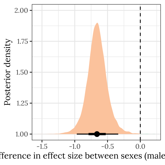

Version	Author	Date
709456c	Martin Garlovsky	2021-01-18
989e86f	lukeholman	2020-12-18
96d1188	Martin Garlovsky	2020-12-13
7d4b609	Martin Garlovsky	2020-12-05
df61dde	Martin Garlovsky	2020-12-04

Table

treatsex_interaction_eclosion <- treatsex_eclosion %>%
  select(draw, SEX, d =  `Difference in means (Poly - Mono)`) %>%
  arrange(draw, SEX) %>%
  group_by(draw) %>%
  summarise(`Difference in effect size between sexes (male - female)` = d[2] - d[1],
            .groups = "drop") # males - females

treatsex_interaction_eclosion %>%
  rename(x = `Difference in effect size between sexes (male - female)`) %>%
  summarise(`Difference in effect size between sexes (male - female)` = median(x),
            `Lower 95% CI` = quantile(x, probs = 0.025), 
            `Upper 95% CI` = quantile(x, probs = 0.975),
            p = 1 - as.numeric(bayestestR::p_direction(x)),
            ` ` = ifelse(p < 0.05, "\\*", ""),
            .groups = "drop") %>%
  kable(digits=3) %>%
  kable_styling(full_width = FALSE)

Difference in effect size between sexes (male - female)	Lower 95% CI	Upper 95% CI	p
-0.661	-0.969	-0.337	0.001	*

sex_eclosion <- posterior_samples(cox_brm) %>% 
  as_tibble() %>%
  select(starts_with("b_")) %>% 
  mutate(draw = 1:n()) %>% 
  mutate(M_f = b_Intercept,
         P_f = b_Intercept + b_TRTP,
         M_m = b_Intercept + b_SEXm,
         P_m = b_TRTP + b_SEXm + `b_TRTP:SEXm`) %>% 
  select(draw, M_f, P_f, M_m, P_m) %>% 
  pivot_longer(cols = 2:5) %>% 
  mutate(SEX = str_sub(name, -1),
         TRT = str_sub(name, 1, 1)) %>%
  select(draw, value, SEX, TRT) %>% 
  pivot_wider(names_from = SEX,
              values_from = value) %>%
  mutate(`Difference in means (Female - Male)` = f - m)

sex_eclosion %>%
  ggplot(aes(x = TRT, y = `Difference in means (Female - Male)`, fill = TRT)) +
  #geom_hline(yintercept = 0, linetype = 2) +
  stat_halfeye() + 
  scale_fill_brewer(palette = 'Pastel1', direction = 1, name = "") +
  scale_colour_brewer(palette = 'Pastel1', direction = 1, name = "") +
  labs(y = 'Difference in means (\u03b2) between\nsexess (Female - Male)') +
  theme_bw() +
  theme(legend.position = 'none',
        strip.background = element_blank(),
        panel.grid.major.x = element_blank()) +
  NULL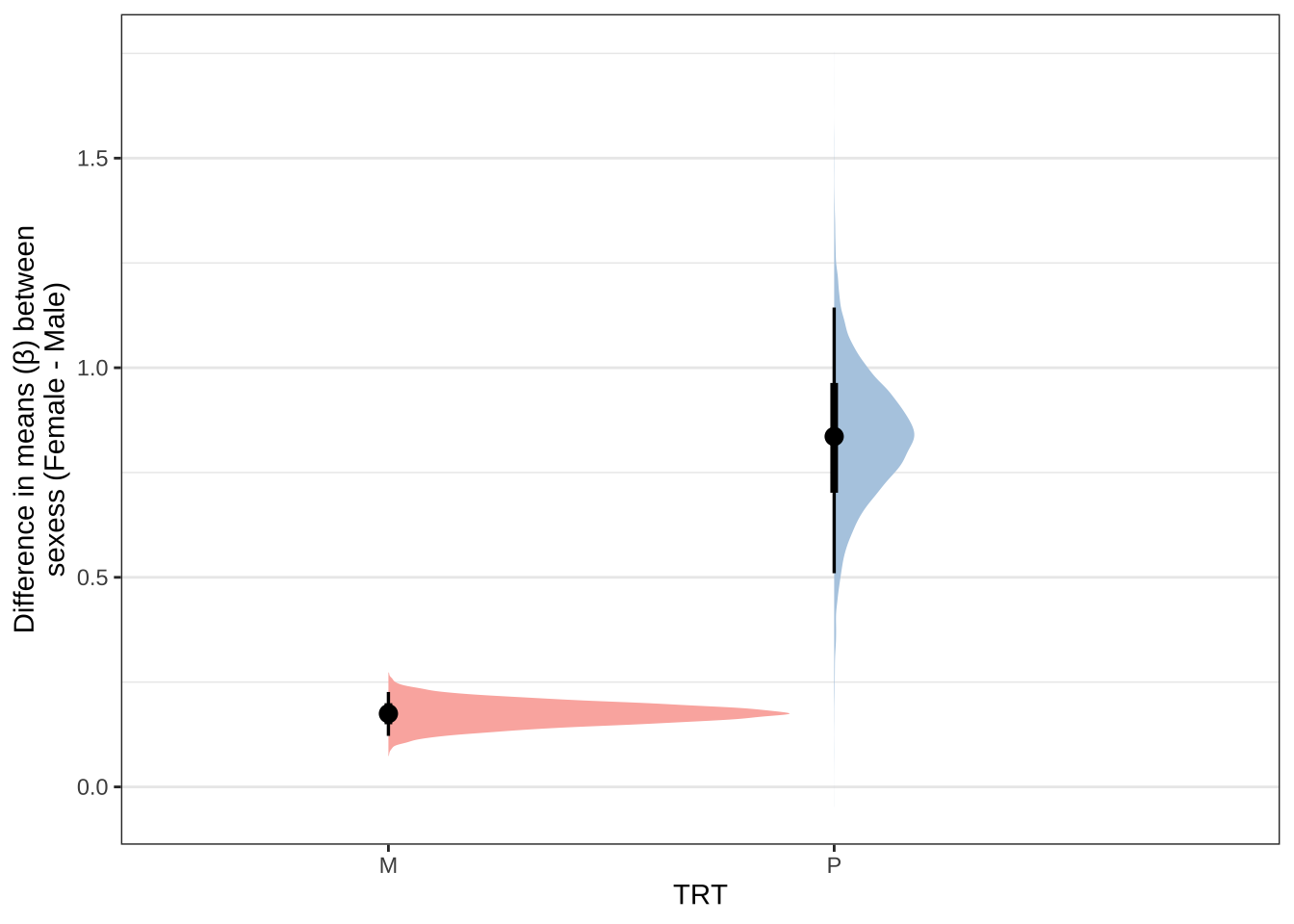

Version	Author	Date
709456c	Martin Garlovsky	2021-01-18
989e86f	lukeholman	2020-12-18
96d1188	Martin Garlovsky	2020-12-13

Body size differences (wing vein IV length)

We measured the length of wing vein VI as a proxy for body size to test for differences between sexes and treatments as body size may influence development time. Prior to measurement, wing images were anonymised using a custom python script provided by Henry Barton and then decoded for statistical analysis. Wing length was scaled by subtracting the mean (across all measurements) and dividing by the standard deviation.

Inspecting the raw data

Violin plots

wing_length %>% 
  mutate(var = paste(Treatment, Sex)) %>% 
  ggplot(aes(x = Sex, y = Length)) +
  geom_violin(aes(fill = var), alpha = .5) + 
  geom_boxplot(aes(fill = var), width = .1, position = position_dodge(width = .9)) +
  scale_colour_manual(values = c("pink", "skyblue", "red", "blue"), name = "") +
  scale_fill_manual(values = c("pink", "skyblue", "red", "blue"), name = "",
                    labels = c('Monogamy Females', 'Monogamy Males',
                               'Polandry Females', 'Polandry Males')) +
  labs(y = 'Wing vein IV length') +
  theme_bw() +
  theme() +
  NULL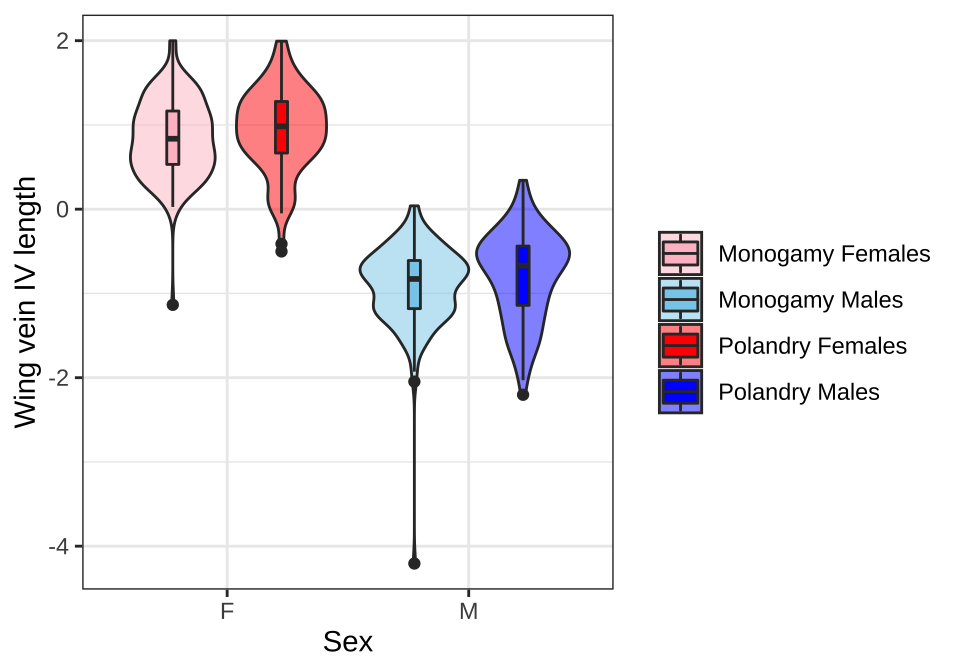

Version	Author	Date
709456c	Martin Garlovsky	2021-01-18
989e86f	lukeholman	2020-12-18
96d1188	Martin Garlovsky	2020-12-13
7d4b609	Martin Garlovsky	2020-12-05

Figure X: Wing vein IV length has been scaled (subtracted the mean and divided by the standard deviation).

Means and standard errors

wing_length %>% 
  group_by(Treatment, Sex) %>% 
  summarise(Mean = mean(Length),
            `Std. Errors` = sd(Length)/sqrt(n()),
            N = n()) %>%
  mutate(Treatment = recode(Treatment, M = "Monogamy", P = 'Polyandry'),
         Sex = recode(Sex, M = "Male", F = 'Female')) %>% 
  mutate(across(2:4, round, 2)) %>% 
  kable() %>% 
  kable_styling(full_width = FALSE)

Treatment	Sex	Mean	Std. Errors	N
Monogamy	Female	0.85	0.04	152
Monogamy	Male	-0.91	0.04	154
Polyandry	Female	0.94	0.05	118
Polyandry	Male	-0.79	0.05	127

Fitting the model for wing length in `brms`

We fit a model in brms to test for differences in wing length between the sexes and sexual selection treatments. We fit treatment, sex and the treatment x sex interaction as fixed effects as well as Seed day as a covariate. As above, we included replicate treatment as a random intercept for each of the 8 lines and a random slope term for selection to allow the effect of treatment to vary across replicate lines.

Define priors

As above we set conservative normal priors on the fixed effects (mean = 0, sd = 1) and half Cauchy priors on the random effects - LINE - (mean = 0, scale = 0.1). All other priors were left at the default in brms.

Run the model

The model is run over 4 chains with 10000 iterations each (with the first 2500 discarded as burn-in), for a total of 7500*4 = 30,000 posterior samples.

if(!file.exists("output/wing_brms.rds")){
  
  wing_brms <- brm(Length ~ Treatment * Sex + Seed + (Treatment|LINE),
                 data = wing_length,
  iter = 10000, chains = 4, cores = 4,
  prior = c(set_prior("normal(0,1)", class = "b"),
            set_prior("cauchy(0,0.1)", class = "sd")),
  control = list(max_treedepth = 20,
                 adapt_delta = 0.999)
  )
  
  saveRDS(wing_brms, "output/wing_brms.rds")
} else {
  wing_brms <- readRDS('output/wing_brms.rds')
}

Posterior predictive check of model fit

pp_check(wing_brms)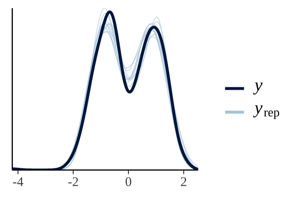

Version	Author	Date
989e86f	lukeholman	2020-12-18
96d1188	Martin Garlovsky	2020-12-13

Table of model parameter estimates - body size

Formatted table

wing_test <- bind_rows(
  hypothesis(wing_brms, 'TreatmentP = 0')$hypothesis,
  hypothesis(wing_brms, 'SexM = 0')$hypothesis,
  hypothesis(wing_brms, 'TreatmentP:SexM = 0')$hypothesis,
  hypothesis(wing_brms, 'SeedB = 0')$hypothesis,
  hypothesis(wing_brms, 'SeedC = 0')$hypothesis,
) %>% 
  mutate(Parameter = c('Treatment (E)', 'Sex (M)', 'Treatment (E) x Sex (M)',
                       'Seed (B)', 'Seed (C)'),
         across(2:5, round, 3)) %>% 
  relocate(Parameter, Estimate, Est.Error, CI.Lower, CI.Upper, Star)

pvals <- bayestestR::p_direction(wing_brms) %>% 
  as.data.frame() %>%
  mutate(vars = map_chr(str_split(Parameter, "_"), ~ .x[2]),
         p_val = 1 - pd, 
         star = ifelse(p_val < 0.05, "\\*", "")) %>%
  select(vars, p_val, star)

wing_test %>% mutate(vars = c('TreatmentP', 'SexM', 'TreatmentP.SexM', 'SeedB', 'SeedC')) %>% 
  left_join(pvals %>% filter(vars != 'Intercept'), 
              by = c("vars")) %>% 
    select(Parameter, Estimate, Est.Error, CI.Lower, CI.Upper, `p` = p_val, star) %>% 
  mutate(p = ifelse(p > 0.001, round(p, 3), '< 0.001')) %>% 
  rename(` ` = star) %>%
  kable() %>% 
  kable_styling(full_width = FALSE)

Parameter	Estimate	Est.Error	CI.Lower	CI.Upper	p
Treatment (E)	0.111	0.261	-0.406	0.638	0.317
Sex (M)	-1.733	0.045	-1.823	-1.644	< 0.001	*
Treatment (E) x Sex (M)	0.020	0.068	-0.114	0.154	0.384
Seed (B)	-0.098	0.042	-0.181	-0.017	0.008	*
Seed (C)	-0.030	0.043	-0.115	0.054	0.24

Complete output from `summary.brmsfit()`

wing_brms

 Family: gaussian 
  Links: mu = identity; sigma = identity 
Formula: Length ~ Treatment * Sex + Seed + (Treatment | LINE) 
   Data: wing_length (Number of observations: 551) 
Samples: 4 chains, each with iter = 10000; warmup = 5000; thin = 1;
         total post-warmup samples = 20000

Group-Level Effects: 
~LINE (Number of levels: 8) 
                          Estimate Est.Error l-95% CI u-95% CI Rhat Bulk_ESS
sd(Intercept)                 0.33      0.12     0.16     0.61 1.00     7540
sd(TreatmentP)                0.16      0.18     0.00     0.65 1.00     6252
cor(Intercept,TreatmentP)     0.09      0.55    -0.91     0.95 1.00    15048
                          Tail_ESS
sd(Intercept)                10324
sd(TreatmentP)                7152
cor(Intercept,TreatmentP)    10995

Population-Level Effects: 
                Estimate Est.Error l-95% CI u-95% CI Rhat Bulk_ESS Tail_ESS
Intercept           0.87      0.18     0.51     1.22 1.00     8584     9556
TreatmentP          0.11      0.26    -0.41     0.64 1.00    10015    10628
SexM               -1.73      0.05    -1.82    -1.64 1.00    20172    15736
SeedB              -0.10      0.04    -0.18    -0.02 1.00    22473    15468
SeedC              -0.03      0.04    -0.11     0.05 1.00    22268    15614
TreatmentP:SexM     0.02      0.07    -0.11     0.15 1.00    19758    15712

Family Specific Parameters: 
      Estimate Est.Error l-95% CI u-95% CI Rhat Bulk_ESS Tail_ESS
sigma     0.40      0.01     0.37     0.42 1.00    26769    14763

Samples were drawn using sampling(NUTS). For each parameter, Bulk_ESS
and Tail_ESS are effective sample size measures, and Rhat is the potential
scale reduction factor on split chains (at convergence, Rhat = 1).

Posterior effect size of treatment on body size for each sex

We predict the mean wing vein IV length for each treatment and sex from the model averaged across the eight replicate selection lines and seeding days. The plots show the difference in posterior estimates between the E and M treatment for each sex separately. Note that females are larger than males but effect sizes are plotted for each sex separately.

new <- expand_grid(Sex = c("M", "F"),
                   Treatment = c("M", "P"),
                   LINE = NA, Seed = NA) %>%
  mutate(type = 1:n())

fitted_wing <- posterior_epred(
  wing_brms, newdata = new, re_formula = NA,
  summary = FALSE, resp = 'Length') %>%
  reshape2::melt() %>% rename(draw = Var1, type = Var2) %>%
  as_tibble() %>%
  left_join(new, by = "type") %>%
  select(draw, value, Sex, Treatment)

treat_diff_wing <- fitted_wing %>%
  spread(Treatment, value) %>%
  mutate(`Difference in means (Poly - Mono)` = P - M) 

treat_diff_wing %>% 
  ggplot(aes(x = Sex, y = `Difference in means (Poly - Mono)`, fill = Sex)) +
  geom_hline(yintercept = 0, linetype = 2) +
  stat_halfeye() + 
  scale_fill_brewer(palette = 'Pastel1', direction = 1, name = "") +
  scale_colour_brewer(palette = 'Pastel1', direction = 1, name = "") +
  labs(y = 'Difference in means between\nselection treatments (E - M)') +
  theme_bw() +
  theme(legend.position = 'none',
        strip.background = element_blank(),
        panel.grid.major.x = element_blank()) +
  NULL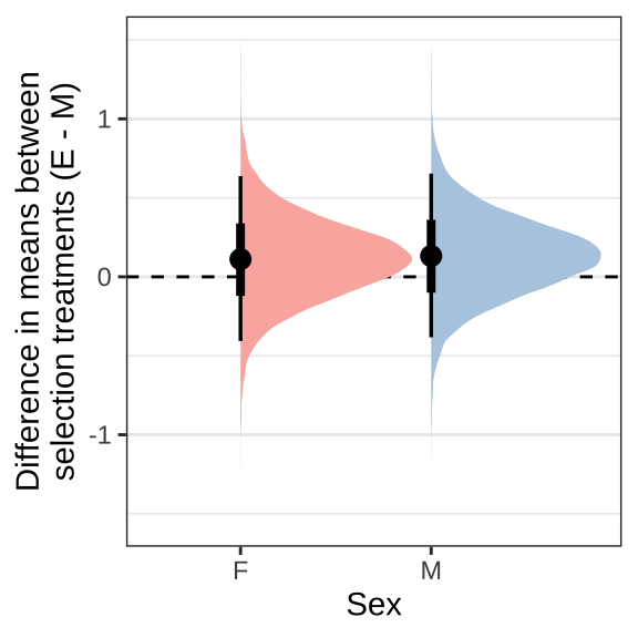

Figure XX: Posterior estimates of treatment effects on wing vein IV length (proxy for body size).

Posterior difference in treatment effect size between sexes

This section examines the treatment \(\times\) sex interaction term, by calculating the difference in the effect size of the E/M treatment between sexes. We find no evidence for a treatment \(\times\) sex interaction, i.e. the treatment effects did not differ detectably between sexes.

Figure

treat_diff_wing %>%
  rename(d = `Difference in means (Poly - Mono)`) %>% 
  select(draw, Sex, d) %>%
  group_by(draw) %>%
  summarise(`Difference in effect size between sexes (male - female)` = d[2] - d[1],
            .groups = "drop") %>% 
  ggplot(aes(x = `Difference in effect size between sexes (male - female)`, y = 1, fill = stat(x < 0))) +
  geom_vline(xintercept = 0, linetype = 2) +
  stat_halfeye() +
  scale_fill_brewer(palette = 'Pastel2', direction = 1, name = "") +
  theme_bw() +
  theme(legend.position = 'none',
        text = element_text(family = nice_font),
        strip.background = element_blank()) +
  ylab("Posterior density") +
  #ggsave("figures/wing_interaction_plot.pdf", height=4, width=4) +
  NULL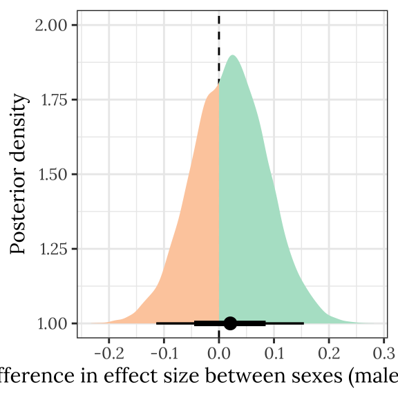

Table

treatsex_interaction_wing <- treat_diff_wing %>%
  select(draw, Sex, d =  `Difference in means (Poly - Mono)`) %>%
  arrange(draw, Sex) %>%
  group_by(draw) %>%
  summarise(`Difference in effect size between sexes (male - female)` = d[2] - d[1],
            .groups = "drop") # males - females

treatsex_interaction_wing %>%
  rename(x = `Difference in effect size between sexes (male - female)`) %>%
  summarise(`Difference in effect size between sexes (male - female)` = median(x),
            `Lower 95% CI` = quantile(x, probs = 0.025), 
            `Upper 95% CI` = quantile(x, probs = 0.975),
            p = 1 - as.numeric(bayestestR::p_direction(x)),
            ` ` = ifelse(p < 0.05, "\\*", ""),
            .groups = "drop") %>%
  kable(digits=3) %>%
  kable_styling(full_width = FALSE)

Difference in effect size between sexes (male - female)	Lower 95% CI	Upper 95% CI	p
0.021	-0.114	0.154	0.384

sessionInfo()

R version 4.0.3 (2020-10-10)
Platform: x86_64-apple-darwin17.0 (64-bit)
Running under: macOS Big Sur 10.16

Matrix products: default
BLAS:   /Library/Frameworks/R.framework/Versions/4.0/Resources/lib/libRblas.dylib
LAPACK: /Library/Frameworks/R.framework/Versions/4.0/Resources/lib/libRlapack.dylib

locale:
[1] en_GB.UTF-8/en_GB.UTF-8/en_GB.UTF-8/C/en_GB.UTF-8/en_GB.UTF-8

attached base packages:
[1] stats     graphics  grDevices utils     datasets  methods   base     

other attached packages:
 [1] showtext_0.9-2   showtextdb_3.0   sysfonts_0.8.3   knitrhooks_0.0.4
 [5] knitr_1.31       kableExtra_1.3.1 tidybayes_2.3.1  brms_2.14.4     
 [9] Rcpp_1.0.6       coxme_2.2-16     bdsmatrix_1.3-4  survival_3.2-7  
[13] ggridges_0.5.3   forcats_0.5.1    stringr_1.4.0    dplyr_1.0.3     
[17] purrr_0.3.4      readr_1.4.0      tidyr_1.1.2      tibble_3.0.5    
[21] ggplot2_3.3.3    tidyverse_1.3.0  workflowr_1.6.2 

loaded via a namespace (and not attached):
  [1] readxl_1.3.1         backports_1.2.1      plyr_1.8.6          
  [4] igraph_1.2.6         splines_4.0.3        svUnit_1.0.3        
  [7] crosstalk_1.1.1      rstantools_2.1.1     inline_0.3.17       
 [10] digest_0.6.27        htmltools_0.5.1.1    rsconnect_0.8.16    
 [13] fansi_0.4.2          magrittr_2.0.1       openxlsx_4.2.3      
 [16] modelr_0.1.8         RcppParallel_5.0.2   matrixStats_0.57.0  
 [19] xts_0.12.1           prettyunits_1.1.1    colorspace_2.0-0    
 [22] rvest_0.3.6          ggdist_2.4.0         haven_2.3.1         
 [25] xfun_0.20            callr_3.5.1          crayon_1.3.4        
 [28] jsonlite_1.7.2       lme4_1.1-26          zoo_1.8-8           
 [31] glue_1.4.2           survminer_0.4.8      gtable_0.3.0        
 [34] webshot_0.5.2        V8_3.4.0             distributional_0.2.1
 [37] car_3.0-10           pkgbuild_1.2.0       rstan_2.21.1        
 [40] abind_1.4-5          scales_1.1.1         mvtnorm_1.1-1       
 [43] DBI_1.1.1            rstatix_0.6.0        miniUI_0.1.1.1      
 [46] viridisLite_0.3.0    xtable_1.8-4         foreign_0.8-81      
 [49] km.ci_0.5-2          stats4_4.0.3         StanHeaders_2.21.0-7
 [52] DT_0.17              htmlwidgets_1.5.3    httr_1.4.2          
 [55] threejs_0.3.3        RColorBrewer_1.1-2   arrayhelpers_1.1-0  
 [58] ellipsis_0.3.1       reshape_0.8.8        pkgconfig_2.0.3     
 [61] loo_2.4.1            farver_2.0.3         dbplyr_2.0.0        
 [64] labeling_0.4.2       tidyselect_1.1.0     rlang_0.4.10        
 [67] reshape2_1.4.4       later_1.1.0.1        munsell_0.5.0       
 [70] cellranger_1.1.0     tools_4.0.3          cli_2.2.0           
 [73] generics_0.1.0       broom_0.7.3          evaluate_0.14       
 [76] fastmap_1.1.0        yaml_2.2.1           processx_3.4.5      
 [79] fs_1.5.0             zip_2.1.1            survMisc_0.5.5      
 [82] nlme_3.1-151         whisker_0.4          mime_0.9            
 [85] projpred_2.0.2       xml2_1.3.2           compiler_4.0.3      
 [88] bayesplot_1.8.0      shinythemes_1.2.0    rstudioapi_0.13     
 [91] gamm4_0.2-6          curl_4.3             ggsignif_0.6.0      
 [94] reprex_1.0.0         statmod_1.4.35       stringi_1.5.3       
 [97] highr_0.8            ps_1.5.0             Brobdingnag_1.2-6   
[100] lattice_0.20-41      Matrix_1.3-2         nloptr_1.2.2.2      
[103] markdown_1.1         KMsurv_0.1-5         shinyjs_2.0.0       
[106] vctrs_0.3.6          pillar_1.4.7         lifecycle_0.2.0     
[109] bridgesampling_1.0-0 insight_0.12.0       data.table_1.13.6   
[112] httpuv_1.5.5         R6_2.5.0             promises_1.1.1      
[115] rio_0.5.16           gridExtra_2.3        codetools_0.2-18    
[118] boot_1.3-26          colourpicker_1.1.0   MASS_7.3-53         
[121] gtools_3.8.2         assertthat_0.2.1     rprojroot_2.0.2     
[124] withr_2.4.1          shinystan_2.5.0      bayestestR_0.8.2    
[127] mgcv_1.8-33          parallel_4.0.3       hms_1.0.0           
[130] grid_4.0.3           coda_0.19-4          minqa_1.2.4         
[133] rmarkdown_2.6        carData_3.0-4        ggpubr_0.4.0        
[136] git2r_0.28.0         shiny_1.6.0          lubridate_1.7.9.2   
[139] base64enc_0.1-3      dygraphs_1.1.1.6

Juvenile development time

Load packages

Load data

Inspecting the raw data

Survival analysis

Censoring

Kaplan-Meier survival curve

Median eclosion times

Check proportional hazards assumption

Fit the model in brms

Define priors

Run the model

Table of model parameter estimates - eclosion time

Formatted table

Complete output from summary.brmsfit()

Posterior effect size of treatment on eclosion time for each sex

Posterior difference in treatment effect size between sexes

Figure

Table

Body size differences (wing vein IV length)

Inspecting the raw data

Violin plots

Means and standard errors

Fitting the model for wing length in brms

Define priors

Run the model

Posterior predictive check of model fit

Table of model parameter estimates - body size

Formatted table

Complete output from summary.brmsfit()

Posterior effect size of treatment on body size for each sex

Posterior difference in treatment effect size between sexes

Figure

Table

Fit the model in `brms`

Complete output from `summary.brmsfit()`

Fitting the model for wing length in `brms`

Complete output from `summary.brmsfit()`