Last updated: 2020-12-09

Checks: 7 0

Knit directory: exp_evol_respiration/

This reproducible R Markdown analysis was created with workflowr (version 1.6.2). The Checks tab describes the reproducibility checks that were applied when the results were created. The Past versions tab lists the development history.

R Markdown file: up-to-date

Great! Since the R Markdown file has been committed to the Git repository, you know the exact version of the code that produced these results.

Environment: empty

Great job! The global environment was empty. Objects defined in the global environment can affect the analysis in your R Markdown file in unknown ways. For reproduciblity it’s best to always run the code in an empty environment.

Seed: set.seed(20190703)

The command set.seed(20190703) was run prior to running the code in the R Markdown file. Setting a seed ensures that any results that rely on randomness, e.g. subsampling or permutations, are reproducible.

Session information: recorded

Great job! Recording the operating system, R version, and package versions is critical for reproducibility.

Cache: none

Nice! There were no cached chunks for this analysis, so you can be confident that you successfully produced the results during this run.

File paths: relative

Great job! Using relative paths to the files within your workflowr project makes it easier to run your code on other machines.

Repository version: 15f3c92

Great! You are using Git for version control. Tracking code development and connecting the code version to the results is critical for reproducibility.

The results in this page were generated with repository version 15f3c92. See the Past versions tab to see a history of the changes made to the R Markdown and HTML files.

Note that you need to be careful to ensure that all relevant files for the analysis have been committed to Git prior to generating the results (you can use wflow_publish or wflow_git_commit). workflowr only checks the R Markdown file, but you know if there are other scripts or data files that it depends on. Below is the status of the Git repository when the results were generated:


Ignored files:
    Ignored:    .DS_Store
    Ignored:    .Rproj.user/
    Ignored:    analysis/.DS_Store

Note that any generated files, e.g. HTML, png, CSS, etc., are not included in this status report because it is ok for generated content to have uncommitted changes.

These are the previous versions of the repository in which changes were made to the R Markdown (analysis/metabolites.Rmd) and HTML (docs/metabolites.html) files. If you’ve configured a remote Git repository (see ?wflow_git_remote), click on the hyperlinks in the table below to view the files as they were in that past version.

File	Version	Author	Date	Message
Rmd	15f3c92	lukeholman	2020-12-09	Tweaks
html	43cc270	lukeholman	2020-12-09	Build site.
Rmd	2642c27	lukeholman	2020-12-09	More work
html	4f5ee28	lukeholman	2020-12-04	Build site.
Rmd	d441b69	lukeholman	2020-12-04	Luke metabolites analysis
Rmd	c8feb2d	lukeholman	2020-11-30	Same page with Martin
html	3fdbcb2	lukeholman	2020-11-30	Tweaks Nov 2020

Load packages

library(tidyverse)

── Attaching packages ────────────────────────────────────────────────────────────────────────────── tidyverse 1.3.0 ──

✓ ggplot2 3.3.2     ✓ purrr   0.3.4
✓ tibble  3.0.1     ✓ dplyr   1.0.0
✓ tidyr   1.1.0     ✓ stringr 1.4.0
✓ readr   1.3.1     ✓ forcats 0.5.0

── Conflicts ───────────────────────────────────────────────────────────────────────────────── tidyverse_conflicts() ──
x dplyr::filter() masks stats::filter()
x dplyr::lag()    masks stats::lag()

library(GGally)

Registered S3 method overwritten by 'GGally':
  method from   
  +.gg   ggplot2

library(gridExtra)


Attaching package: 'gridExtra'

The following object is masked from 'package:dplyr':

    combine

library(ggridges)
library(brms)

Loading required package: Rcpp

Loading 'brms' package (version 2.14.4). Useful instructions
can be found by typing help('brms'). A more detailed introduction
to the package is available through vignette('brms_overview').


Attaching package: 'brms'

The following object is masked from 'package:stats':

    ar

library(tidybayes)


Attaching package: 'tidybayes'

The following objects are masked from 'package:ggridges':

    scale_point_color_continuous, scale_point_color_discrete, scale_point_colour_continuous, scale_point_colour_discrete,
    scale_point_fill_continuous, scale_point_fill_discrete, scale_point_size_continuous

library(DT)
library(kableExtra)


Attaching package: 'kableExtra'

The following object is masked from 'package:dplyr':

    group_rows

library(knitrhooks) # install with devtools::install_github("nathaneastwood/knitrhooks")

Loading required package: knitr

output_max_height() # a knitrhook option

options(stringsAsFactors = FALSE)

Load metabolite composition data

This analysis set out to test whether sexual selection treatment had an effect on metabolite composition of flies. We measured fresh and dry fly weight in milligrams, plus the weights of five metabolites which together equal the dry weight. These are:

Lipid_conc (i.e. the weight of the hexane fraction, divided by the full dry weight),
Carbohydrate_conc (i.e. the weight of the aqueous fraction, divided by the full dry weight),
Protein_conc (i.e. \(\mu\)g of protein per milligram as measured by the bicinchoninic acid protein assay),
Glycogen_conc (i.e. \(\mu\)g of glycogen per milligram as measured by the hexokinase assay), and
Chitin_conc (estimated as the difference between the initial and final dry weights)

We expect body weight to vary between the sexes and potentially between treatments. In turn, we expect body weight to affect our five response variables of interest. Larger flies will have more lipids, carbs, etc., and this may vary by sex and treatment both directly and indirectly.

metabolites <- read_csv('data/3.metabolite_data.csv') %>%
  mutate(sex = ifelse(sex == "m", "Male", "Female"),
         line = paste(treatment, line, sep = ""),
         treatment = ifelse(treatment == "M", "Monogamy", "Polyandry")) %>%
  # log transform glycogen since it shows a long tail (others are reasonably normal-looking)
  mutate(Glycogen_ug_mg = log(Glycogen_ug_mg)) %>%
  # There was a technical error with flies collected on day 1, 
  # so they are excluded from the whole paper. All the measurements analysed are of 3d-old flies
  filter(time == '2') %>%
  select(-time)

Parsed with column specification:
cols(
  sex = col_character(),
  treatment = col_character(),
  line = col_double(),
  time = col_double(),
  fwt_mg = col_double(),
  dwt_mg = col_double(),
  Hex_frac = col_double(),
  p_hex_frac = col_double(),
  Aq_frac = col_double(),
  p_Aq_frac = col_double(),
  Protein = col_double(),
  Protein_ug_mg = col_double(),
  Glycogen = col_double(),
  Glycogen_ug_mg = col_double(),
  Chitin = col_double(),
  Chitin_mg_mg = col_double()
)

scaled_metabolites <- metabolites %>% 
  # Find proportional metabolites as a proportion of total dry weight
  mutate(
    Dry_weight = dwt_mg,
    Lipid_conc = Hex_frac / Dry_weight,
    Carbohydrate_conc = Aq_frac / Dry_weight,
    Protein_conc = Protein_ug_mg,
    Glycogen_conc = Glycogen_ug_mg,
    Chitin_conc = Chitin_mg_mg) %>% 
  select(sex, treatment, line, Dry_weight, ends_with("conc")) %>%
  mutate_at(vars(ends_with("conc")), ~ as.numeric(scale(.x))) %>%
  mutate(Dry_weight = as.numeric(scale(Dry_weight))) %>%
  mutate(sextreat = paste(sex, treatment),
         sextreat = replace(sextreat, sextreat == "Male Monogamy", "M males"),
         sextreat = replace(sextreat, sextreat == "Male Polyandry", "P males"),
         sextreat = replace(sextreat, sextreat == "Female Monogamy", "M females"),
         sextreat = replace(sextreat, sextreat == "Female Polyandry", "P females"),
         sextreat = factor(sextreat, c("M males", "P males", "M females", "P females")))

Inspect the raw data

Raw numbers

All variables are shown in standard units (i.e. mean = 0, SD = 1).

my_data_table <- function(df){
  datatable(
    df, rownames=FALSE,
    autoHideNavigation = TRUE,
    extensions = c("Scroller",  "Buttons"),
    options = list(
      dom = 'Bfrtip',
      deferRender=TRUE,
      scrollX=TRUE, scrollY=400,
      scrollCollapse=TRUE,
      buttons = 
        list('csv', list(
          extend = 'pdf',
          pageSize = 'A4',
          orientation = 'landscape',
          filename = 'Apis_methylation')),
      pageLength = 50
    )
  )
}

scaled_metabolites %>%
  select(-sextreat) %>%
  mutate_if(is.numeric, ~ format(round(.x, 3), nsmall = 3)) %>%
  my_data_table()

Simple plots

The following plot shows how each metabolite varies between sexes and treatments, and how the consecration of each metabolite co-varies with dry weight across individuals.

levels <- c("Carbohydrate", "Chitin", "Glycogen", "Lipid", "Protein", "Dryweight")

cols <- c("M females" = "pink", 
          "P females" = "red", 
          "M males" = "skyblue", 
          "P males" = "blue")

grid.arrange(
  scaled_metabolites %>% 
    rename_all(~ str_remove_all(.x, "_conc")) %>%
    mutate(sex = factor(sex, c("Male", "Female"))) %>%
    reshape2::melt(id.vars = c('sex', 'treatment', 'sextreat', 'line', 'Dry_weight')) %>% 
    mutate(variable = factor(variable, levels)) %>%
    ggplot(aes(x = sex, y = value,  fill  = sextreat)) +
    geom_hline(yintercept = 0, linetype = 2) + 
    geom_boxplot() + 
    facet_grid( ~ variable) +
    theme_bw() +
    xlab("Sex") + ylab("Concentration") +
    theme(legend.position = 'top') + 
    scale_fill_manual(values = cols, name = ""),
  
  scaled_metabolites %>% 
    rename_all(~ str_remove_all(.x, "_conc")) %>%
    reshape2::melt(id.vars = c('sex', 'treatment', 'sextreat', 'line', 'Dry_weight')) %>% 
    mutate(variable = factor(variable, levels)) %>%
    ggplot(aes(x = Dry_weight, y = value, colour = sextreat, fill = sextreat)) +
    geom_smooth(method = 'lm', se = TRUE, aes(colour = NULL, fill = NULL), colour = "grey20", size = .4) +
    geom_point(pch = 21, colour = "grey20") +
    facet_grid( ~ variable) +
    theme_bw() +
    xlab("Dry weight (mg)") + ylab("Concentration") +
    theme(legend.position = 'none') + 
    scale_colour_manual(values = cols, name = "") + 
    scale_fill_manual(values = cols, name = ""),
  heights = c(0.55, 0.45)
)

`geom_smooth()` using formula 'y ~ x'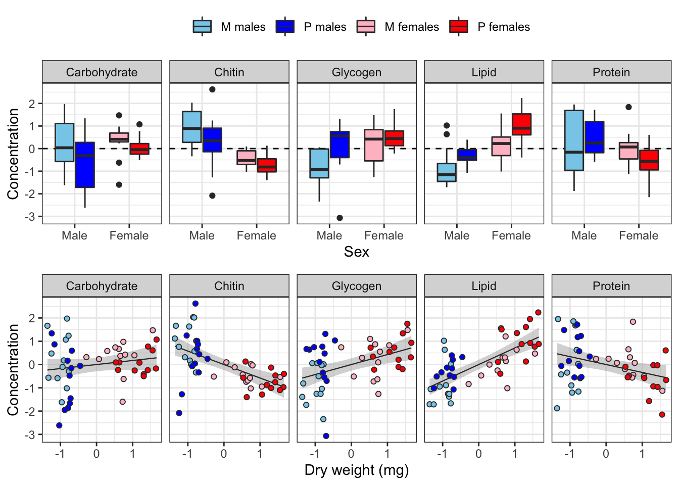

Version	Author	Date
43cc270	lukeholman	2020-12-09
4f5ee28	lukeholman	2020-12-04

Plot of correlations between variables

Some of the metabolites, especially lipid concentration, are correlated with dry weight. There is also a large difference in dry weight between sexes (and treatments, to a less extent), and sex and treatment effects are evident for some of the metabolites in the raw data. Some of the metabolites are weakly correlated with other metabolites, e.g. lipid and glycogen concentration.

modified_densityDiag <- function(data, mapping, ...) {
  ggally_densityDiag(data, mapping, colour = "grey10", ...) + 
    scale_fill_manual(values = cols) + 
  scale_x_continuous(guide = guide_axis(check.overlap = TRUE))
}

modified_points <- function(data, mapping, ...) {
  ggally_points(data, mapping, pch = 21, colour = "grey10", ...) +
    scale_fill_manual(values = cols) + 
    scale_x_continuous(guide = guide_axis(check.overlap = TRUE))
}

modified_facetdensity <- function(data, mapping, ...) {
  ggally_facetdensity(data, mapping, ...) + 
    scale_colour_manual(values = cols)
}

modified_box_no_facet <- function(data, mapping, ...) {
  ggally_box_no_facet(data, mapping, colour = "grey10", ...) +
    scale_fill_manual(values = cols)
}

pairs_plot <- scaled_metabolites %>% 
  arrange(sex, treatment) %>%
  select(-line, -sex, -treatment) %>%
  rename(`Sex and treatment` = sextreat) %>%
  rename_all(~ str_replace_all(.x, "_", " ")) %>%
  ggpairs(aes(colour = `Sex and treatment`, fill = `Sex and treatment`),
          diag = list(continuous = wrap(modified_densityDiag, alpha = 0.7),
                      discrete = wrap("blank")),
          lower = list(continuous = wrap(modified_points, alpha = 0.7, size = 1.1), 
                       discrete = wrap("blank"),
                       combo = wrap(modified_box_no_facet, alpha = 0.7)),
          upper = list(continuous = wrap(modified_points, alpha = 0.7, size = 1.1),
                       discrete = wrap("blank"),
                       combo = wrap(modified_box_no_facet, alpha = 0.7, size = 0.5))) 
pairs_plot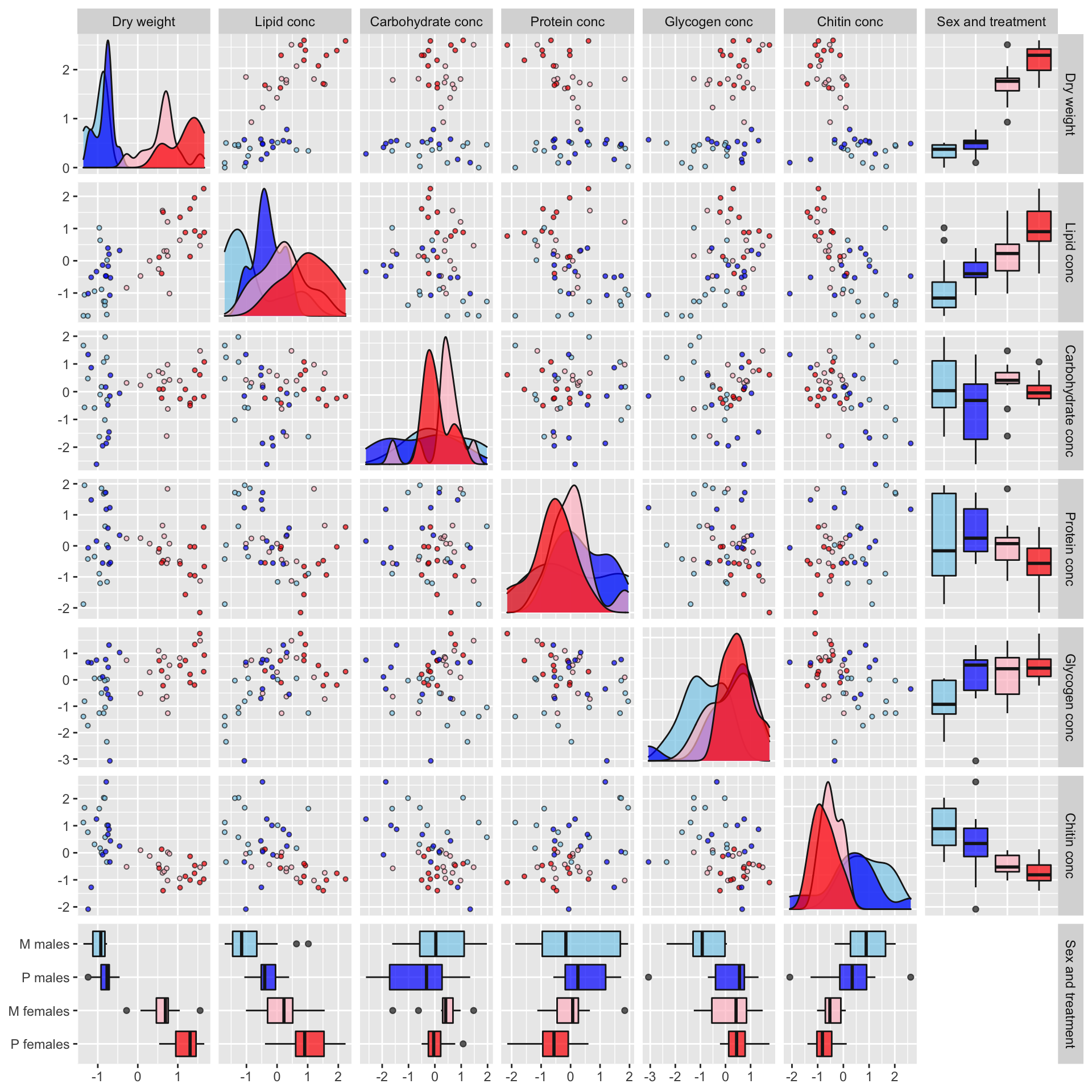

Version	Author	Date
43cc270	lukeholman	2020-12-09

Directed acyclic graph (DAG)

This directed acyclic graph (DAG) illustrates the causal pathways that we observed between the experimental or measured variables (square boxes) and latent variables (ovals). We hypothesise that sex and mating system potentially influence dry weight as well as the metabolite composition (which we assessed by estimating the concentrations of carbohydrates, chitin, glycogen, lipids and protein). Additionally, dry weight is likely correlated with metabolite composition, and so dry weight acts as a ‘mediator variable’ between metabolite composition, and sex and treatment. The structural equation model below is built with this DAG in mind.

DiagrammeR::grViz('digraph {

graph [layout = dot, rankdir = LR]

# define the global styles of the nodes. We can override these in box if we wish
node [shape = rectangle, style = filled, fillcolor = Linen]

"Metabolite\ncomposition" [shape = oval, fillcolor = Beige]

# edge definitions with the node IDs
"Mating system\ntreatment (M vs P)" -> {"Dry weight"}
"Mating system\ntreatment (M vs P)" -> {"Metabolite\ncomposition"} 

"Sex\n(Female vs Male)" -> {"Dry weight"} -> {"Metabolite\ncomposition"}
"Sex\n(Female vs Male)" -> {"Metabolite\ncomposition"}

{"Metabolite\ncomposition"} -> "Carbohydrates"
{"Metabolite\ncomposition"} -> "Chitin"
{"Metabolite\ncomposition"} -> "Glycogen"
{"Metabolite\ncomposition"} -> "Lipids"
{"Metabolite\ncomposition"} -> "Protein"
}')

Fit `brms` structural equation model

Here we fit a model of the five metabolites, which includes dry body weight as a mediator variable. That is, our model estimates the effect of treatment, sex and line (and all the 2- and 3-way interactions) on dry weight, and then estimates the effect of those some predictors (plus dry weight) on the five metabolites. The model assumes that although the different sexes, treatment groups, and lines may differ in their dry weight, the relationship between dry weight and the metabolites does not vary by sex/treatment/line. This assumption was made to constrain the number of parameters in the model, and to reflect out prior beliefs about allometric scaling of metabolites.

Define Priors

We use set Normal priors on all fixed effect parameters, mean = 0, sd = 1, which ‘regularises’ the estimates towards zero – this is conservative (because it makes large posterior effect sizes more improbable), and it also helps the model to converge. Similarly, we set a somewhat conservative half-cauchy prior (mean 0, scale 0.01) on the random effects for line (i.e. we consider large differences between lines – in terms of means and treatment effects – to be possible but improbable). We leave all other priors at the defaults used by brms.

prior1 <- c(set_prior("normal(0, 1)", class = "b", resp = 'Lipid'),
            set_prior("normal(0, 1)", class = "b", resp = 'Carbohydrate'),
            set_prior("normal(0, 1)", class = "b", resp = 'Protein'),
            set_prior("normal(0, 1)", class = "b", resp = 'Glycogen'),
            set_prior("normal(0, 1)", class = "b", resp = 'Chitin'),
            set_prior("normal(0, 1)", class = "b", resp = 'Dryweight'),
            set_prior("cauchy(0,0.01)", class = "sd", resp = 'Lipid', group = "line"),
            set_prior("cauchy(0,0.01)", class = "sd", resp = 'Carbohydrate', group = "line"),
            set_prior("cauchy(0,0.01)", class = "sd", resp = 'Protein', group = "line"),
            set_prior("cauchy(0,0.01)", class = "sd", resp = 'Glycogen', group = "line"),
            set_prior("cauchy(0,0.01)", class = "sd", resp = 'Chitin', group = "line"),
            set_prior("cauchy(0,0.01)", class = "sd", resp = 'Dryweight', group = "line"))

prior1

          prior class coef group         resp dpar nlpar bound source
   normal(0, 1)     b                   Lipid                    user
   normal(0, 1)     b            Carbohydrate                    user
   normal(0, 1)     b                 Protein                    user
   normal(0, 1)     b                Glycogen                    user
   normal(0, 1)     b                  Chitin                    user
   normal(0, 1)     b               Dryweight                    user
 cauchy(0,0.01)    sd       line        Lipid                    user
 cauchy(0,0.01)    sd       line Carbohydrate                    user
 cauchy(0,0.01)    sd       line      Protein                    user
 cauchy(0,0.01)    sd       line     Glycogen                    user
 cauchy(0,0.01)    sd       line       Chitin                    user
 cauchy(0,0.01)    sd       line    Dryweight                    user

Define the six sub-models

The fixed effects formula is sex * treatment + Dryweight (or sex * treatment in the case of the model of dry weight). The random effects part of the formula indicates that the 8 independent selection lines may differ in their means, and that the treatment effect may vary in sign/magnitude between lines. The notation | p | means that the model estimates the correlations in line effects (both slopes and intercepts) between the 6 response variables. Finally, the notation set_rescor(TRUE) means that the model should estimate the residual correlations between the response variables.

brms_formula <- 
  
  # Sub-models of the 5 metabolites
  bf(mvbind(Lipid, Carbohydrate, Protein, Glycogen, Chitin) ~ 
       sex*treatment + Dryweight + (treatment | p | line)) +
  
  # dry weight sub-model
   bf(Dryweight ~ sex*treatment + (treatment | p | line)) +
  
  # Allow for (and estimate) covariance between the residuals of the difference response variables
  set_rescor(TRUE)

brms_formula

Lipid ~ sex * treatment + Dryweight + (treatment | p | line) 
Carbohydrate ~ sex * treatment + Dryweight + (treatment | p | line) 
Protein ~ sex * treatment + Dryweight + (treatment | p | line) 
Glycogen ~ sex * treatment + Dryweight + (treatment | p | line) 
Chitin ~ sex * treatment + Dryweight + (treatment | p | line) 
Dryweight ~ sex * treatment + (treatment | p | line)

Running the model

The model is run over 4 chains with 5000 iterations each (with the first 2500 discarded as burn-in), for a total of 2500*4 = 10,000 posterior samples.

if(!file.exists("output/brms_metabolite_SEM.rds")){
  brms_metabolite_SEM <- brm(
    brms_formula,
    data = scaled_metabolites %>% # brms does not like underscores in variable names
      rename(Dryweight = Dry_weight) %>%
      rename_all(~ gsub("_conc", "", .x)),
    iter = 5000, chains = 4, cores = 1,
    prior = prior1,
    control = list(max_treedepth = 20,
                   adapt_delta = 0.99)
  )
  
  saveRDS(brms_metabolite_SEM, "output/brms_metabolite_SEM.rds")
} else {
  brms_metabolite_SEM <- readRDS('output/brms_metabolite_SEM.rds')
}

Posterior predictive check of model fit

The plot below shows that the fitted model is able to produce posterior predictions that have a similar distribution to the original data, for each of the response variables, which is a necessary condition for the model to be used for statistical inference.

grid.arrange(
  pp_check(brms_metabolite_SEM, resp = "Dryweight") + 
    ggtitle("Dry weight") + theme(legend.position = "none"),
  pp_check(brms_metabolite_SEM, resp = "Lipid") + 
    ggtitle("Lipid") + theme(legend.position = "none"),
  pp_check(brms_metabolite_SEM, resp = "Carbohydrate") + 
    ggtitle("Carbohydrate") + theme(legend.position = "none"),
  pp_check(brms_metabolite_SEM, resp = "Protein") + 
    ggtitle("Protein") + theme(legend.position = "none"),
  pp_check(brms_metabolite_SEM, resp = "Glycogen") + 
    ggtitle("Glycogen") + theme(legend.position = "none"),
  pp_check(brms_metabolite_SEM, resp = "Chitin") + 
    ggtitle("Chitin") + theme(legend.position = "none"),
  nrow = 1
)

Version	Author	Date
43cc270	lukeholman	2020-12-09
4f5ee28	lukeholman	2020-12-04

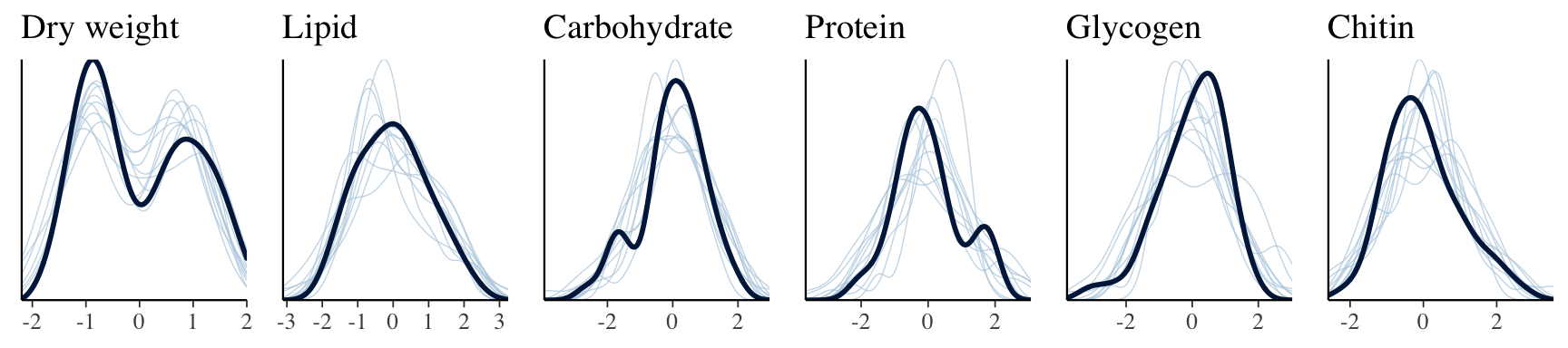
Table of model parameter estimates

Formatted table

This tables shows the fixed effects estimates for the treatment, sex, their interaction, as well as the slope associated with dry weight (where relevant), for each of the six response variables. The p column shows 1 - minus the “probability of direction”, i.e. the posterior probability that the reported sign of the estimate is correct given the data and the prior; subtracting this value from one gives a Bayesian equivalent of a one-sided p-value. For brevity, we have omitted all the parameter estimates involving the predictor variable line, as well as the estimates of residual (co)variance. Click the next tab to see a complete summary of the model and its output.

vars <- c("Lipid", "Carbohydrate", "Glycogen", "Protein", "Chitin")
tests <- c('_Dryweight', '_sexMale',
           '_sexMale:treatmentPolyandry',
           '_treatmentPolyandry')

hypSEM <- data.frame(expand_grid(vars, tests) %>% 
                       mutate(est = NA,
                              err = NA,
                              lwr = NA,
                              upr = NA) %>% 
                       # bind body weight on the end
                       rbind(data.frame(
                         vars = rep('Dryweight', 3),
                         tests = c('_sexMale', 
                                   '_treatmentPolyandry', 
                                   '_sexMale:treatmentPolyandry'),
                         est = NA,
                         err = NA,
                         lwr = NA,
                         upr = NA)))

for(i in 1:nrow(hypSEM)) {
  
  result = hypothesis(brms_metabolite_SEM, 
                      paste0(hypSEM[i, 1], hypSEM[i, 2], ' = 0'))$hypothesis

  hypSEM[i, 3] = round(result$Estimate, 3)
  hypSEM[i, 4] = round(result$Est.Error, 3)
  hypSEM[i, 5] = round(result$CI.Lower, 3)
  hypSEM[i, 6] = round(result$CI.Upper, 3)

}

pvals <- bayestestR::p_direction(brms_metabolite_SEM) %>% 
  as.data.frame() %>%
  mutate(vars = map_chr(str_split(Parameter, "_"), ~ .x[2]),
         tests = map_chr(str_split(Parameter, "_"), ~ .x[3]),
         tests = str_c("_", str_remove_all(tests, "[.]")),
         tests = replace(tests, tests == "_sexMaletreatmentPolyandry", "_sexMale:treatmentPolyandry")) %>%
  filter(!str_detect(tests, "line")) %>%
  mutate(p_val = 1 - pd, star = ifelse(p_val < 0.05, "*", "")) %>%
  select(vars, tests, p_val, star)


hypSEM <- hypSEM %>% left_join(pvals, by = c("vars", "tests"))

hypSEM  %>% 
  mutate(Parameter = c(rep(c('Dry weight', 'Sex (M)', 
                             'Sex (M) x Treatment (P)', 
                             'Treatment (P)'), 5), 
                       'Sex (M)', 'Treatment (P)', 'Sex (M) x Treatment (P)'))  %>% 
  mutate(Parameter = factor(Parameter, c("Dry weight", "Sex (M)", "Treatment (P)", "Sex (M) x Treatment (P)")),
         vars = factor(vars, c("Carbohydrate", "Chitin", "Glycogen", "Lipid", "Protein", "Dryweight"))) %>%
  arrange(vars, Parameter) %>%
  select(Parameter, Estimate = est, `Est. error` = err, 
         `CI lower` = lwr, `CI upper` = upr, `p` = p_val, star) %>% 
  rename(` ` = star) %>%
  kable() %>% 
  kable_styling(full_width = FALSE) %>%
  group_rows("Carbohydrates", 1, 4) %>%
  group_rows("Chitin", 5, 8) %>%
  group_rows("Glycogen", 9, 12) %>%
  group_rows("Lipids", 13, 16) %>% 
  group_rows("Protein", 17, 20) %>% 
  group_rows("Dry weight", 21, 23)

Parameter	Estimate	Est. error	CI lower	CI upper	p
Carbohydrates
Dry weight	0.159	0.485	-0.781	1.115	0.3740
Sex (M)	0.128	0.789	-1.416	1.671	0.4367
Treatment (P)	-0.314	0.449	-1.183	0.555	0.2371
Sex (M) x Treatment (P)	-0.472	0.509	-1.461	0.536	0.1705
Chitin
Dry weight	-0.471	0.465	-1.387	0.423	0.1566
Sex (M)	0.552	0.763	-0.966	2.026	0.2335
Treatment (P)	-0.064	0.399	-0.822	0.745	0.4348
Sex (M) x Treatment (P)	-0.448	0.451	-1.347	0.432	0.1577
Glycogen
Dry weight	0.335	0.468	-0.571	1.243	0.2383
Sex (M)	-0.430	0.770	-1.906	1.104	0.2852
Treatment (P)	0.175	0.412	-0.625	0.976	0.3353
Sex (M) x Treatment (P)	0.604	0.484	-0.367	1.552	0.1054
Lipids
Dry weight	0.610	0.446	-0.256	1.488	0.0868
Sex (M)	-0.025	0.728	-1.455	1.375	0.4873
Treatment (P)	0.437	0.382	-0.314	1.189	0.1215
Sex (M) x Treatment (P)	-0.034	0.419	-0.875	0.777	0.4677
Protein
Dry weight	-0.222	0.470	-1.145	0.707	0.3151
Sex (M)	-0.128	0.776	-1.617	1.417	0.4367
Treatment (P)	-0.378	0.441	-1.232	0.484	0.1913
Sex (M) x Treatment (P)	0.586	0.517	-0.434	1.584	0.1258
Dry weight
Sex (M)	-1.591	0.141	-1.864	-1.312	0.0000
Treatment (P)	0.546	0.157	0.233	0.848	0.0012
Sex (M) x Treatment (P)	-0.395	0.195	-0.779	-0.012	0.0223

Complete output from `summary.brmsfit()`

‘Group-Level Effects’ (also called random effects): This shows the (co)variances associated with the line-specific intercepts (which have names like sd(Lipid_Intercept)) and slopes (e.g. sd(Dryweight_treatmentPolyandry)), as well as the correlations between these effects (e.g. cor(Lipid_Intercept,Protein_Intercept) is the correlation in line effects on lipids and proteins)
‘Population-Level Effects:’ (also called fixed effects): These give the estimates of the intercept (i.e. for female M flies) and the effects of treatment, sex, dry weight, and the treatment \(\times\) sex interaction, for each response variable.
‘Family Specific Parameters’: This is the parameter sigma for the residual variance for each response variable
‘Residual Correlations:’ This give the correlations between the residuals for each pairs of response variables.

Note that the model has converged (Rhat = 1) and the posterior is adequately samples (high ESS values).

brms_metabolite_SEM

 Family: MV(gaussian, gaussian, gaussian, gaussian, gaussian, gaussian) 
  Links: mu = identity; sigma = identity
         mu = identity; sigma = identity
         mu = identity; sigma = identity
         mu = identity; sigma = identity
         mu = identity; sigma = identity
         mu = identity; sigma = identity 
Formula: Lipid ~ sex * treatment + Dryweight + (treatment | p | line) 
         Carbohydrate ~ sex * treatment + Dryweight + (treatment | p | line) 
         Protein ~ sex * treatment + Dryweight + (treatment | p | line) 
         Glycogen ~ sex * treatment + Dryweight + (treatment | p | line) 
         Chitin ~ sex * treatment + Dryweight + (treatment | p | line) 
         Dryweight ~ sex * treatment + (treatment | p | line) 
   Data: scaled_metabolites %>% rename(Dryweight = Dry_weig (Number of observations: 48) 
Samples: 4 chains, each with iter = 5000; warmup = 2500; thin = 1;
         total post-warmup samples = 10000

Group-Level Effects: 
~line (Number of levels: 8) 
                                                                  Estimate Est.Error l-95% CI u-95% CI Rhat Bulk_ESS Tail_ESS
sd(Lipid_Intercept)                                                   0.09      0.15     0.00     0.51 1.00     2095     2341
sd(Lipid_treatmentPolyandry)                                          0.03      0.07     0.00     0.22 1.00    13332     6125
sd(Carbohydrate_Intercept)                                            0.07      0.14     0.00     0.52 1.00     3623     2636
sd(Carbohydrate_treatmentPolyandry)                                   0.05      0.14     0.00     0.47 1.00     8612     4337
sd(Protein_Intercept)                                                 0.06      0.13     0.00     0.47 1.00     5854     3298
sd(Protein_treatmentPolyandry)                                        0.03      0.08     0.00     0.23 1.00    16484     6105
sd(Glycogen_Intercept)                                                0.03      0.07     0.00     0.24 1.00    12198     5266
sd(Glycogen_treatmentPolyandry)                                       0.03      0.06     0.00     0.15 1.00    18288     6178
sd(Chitin_Intercept)                                                  0.07      0.13     0.00     0.47 1.00     3937     3874
sd(Chitin_treatmentPolyandry)                                         0.04      0.11     0.00     0.35 1.00    10361     4796
sd(Dryweight_Intercept)                                               0.05      0.07     0.00     0.25 1.00     3428     5432
sd(Dryweight_treatmentPolyandry)                                      0.03      0.06     0.00     0.21 1.00     8815     5238
cor(Lipid_Intercept,Lipid_treatmentPolyandry)                         0.00      0.28    -0.54     0.55 1.00    26792     7112
cor(Lipid_Intercept,Carbohydrate_Intercept)                           0.01      0.28    -0.53     0.54 1.00    20852     7354
cor(Lipid_treatmentPolyandry,Carbohydrate_Intercept)                 -0.00      0.28    -0.53     0.53 1.00    16765     6360
cor(Lipid_Intercept,Carbohydrate_treatmentPolyandry)                  0.00      0.28    -0.53     0.54 1.00    25816     6812
cor(Lipid_treatmentPolyandry,Carbohydrate_treatmentPolyandry)         0.01      0.28    -0.53     0.54 1.00    17444     7043
cor(Carbohydrate_Intercept,Carbohydrate_treatmentPolyandry)          -0.00      0.28    -0.52     0.54 1.00    12013     6962
cor(Lipid_Intercept,Protein_Intercept)                                0.00      0.28    -0.53     0.53 1.00    27063     7109
cor(Lipid_treatmentPolyandry,Protein_Intercept)                       0.00      0.28    -0.52     0.52 1.00    15083     7506
cor(Carbohydrate_Intercept,Protein_Intercept)                         0.01      0.28    -0.53     0.54 1.00    13647     7267
cor(Carbohydrate_treatmentPolyandry,Protein_Intercept)               -0.00      0.28    -0.54     0.53 1.00    11023     7498
cor(Lipid_Intercept,Protein_treatmentPolyandry)                       0.00      0.28    -0.54     0.53 1.00    29517     6597
cor(Lipid_treatmentPolyandry,Protein_treatmentPolyandry)              0.00      0.28    -0.54     0.54 1.00    17380     6929
cor(Carbohydrate_Intercept,Protein_treatmentPolyandry)               -0.00      0.28    -0.53     0.52 1.00    10970     6920
cor(Carbohydrate_treatmentPolyandry,Protein_treatmentPolyandry)      -0.00      0.28    -0.54     0.54 1.00    10098     6571
cor(Protein_Intercept,Protein_treatmentPolyandry)                     0.00      0.28    -0.53     0.55 1.00     9332     7782
cor(Lipid_Intercept,Glycogen_Intercept)                               0.01      0.28    -0.52     0.54 1.00    27042     6990
cor(Lipid_treatmentPolyandry,Glycogen_Intercept)                      0.00      0.28    -0.53     0.54 1.00    17579     7248
cor(Carbohydrate_Intercept,Glycogen_Intercept)                       -0.00      0.28    -0.54     0.54 1.00    14215     6487
cor(Carbohydrate_treatmentPolyandry,Glycogen_Intercept)              -0.00      0.28    -0.53     0.52 1.00    10812     7605
cor(Protein_Intercept,Glycogen_Intercept)                             0.00      0.28    -0.53     0.53 1.00     8863     7173
cor(Protein_treatmentPolyandry,Glycogen_Intercept)                   -0.00      0.27    -0.53     0.53 1.00     7004     7339
cor(Lipid_Intercept,Glycogen_treatmentPolyandry)                     -0.00      0.27    -0.52     0.53 1.00    25535     7050
cor(Lipid_treatmentPolyandry,Glycogen_treatmentPolyandry)            -0.00      0.28    -0.53     0.52 1.00    18911     6298
cor(Carbohydrate_Intercept,Glycogen_treatmentPolyandry)              -0.00      0.27    -0.52     0.52 1.00    13791     6655
cor(Carbohydrate_treatmentPolyandry,Glycogen_treatmentPolyandry)     -0.00      0.28    -0.54     0.52 1.00    10659     7370
cor(Protein_Intercept,Glycogen_treatmentPolyandry)                   -0.01      0.28    -0.53     0.53 1.00     8603     7328
cor(Protein_treatmentPolyandry,Glycogen_treatmentPolyandry)           0.00      0.28    -0.54     0.53 1.00     7730     7307
cor(Glycogen_Intercept,Glycogen_treatmentPolyandry)                   0.00      0.28    -0.53     0.54 1.00     6596     7278
cor(Lipid_Intercept,Chitin_Intercept)                                 0.00      0.28    -0.54     0.53 1.00    20916     6278
cor(Lipid_treatmentPolyandry,Chitin_Intercept)                       -0.00      0.28    -0.53     0.53 1.00    15610     7353
cor(Carbohydrate_Intercept,Chitin_Intercept)                         -0.00      0.28    -0.53     0.53 1.00    12856     7884
cor(Carbohydrate_treatmentPolyandry,Chitin_Intercept)                -0.01      0.28    -0.55     0.53 1.00    10129     6817
cor(Protein_Intercept,Chitin_Intercept)                               0.00      0.27    -0.51     0.52 1.00     8901     8412
cor(Protein_treatmentPolyandry,Chitin_Intercept)                     -0.00      0.28    -0.54     0.53 1.00     7775     6917
cor(Glycogen_Intercept,Chitin_Intercept)                              0.00      0.28    -0.54     0.54 1.00     6654     7446
cor(Glycogen_treatmentPolyandry,Chitin_Intercept)                     0.00      0.28    -0.53     0.54 1.00     6415     7770
cor(Lipid_Intercept,Chitin_treatmentPolyandry)                       -0.01      0.28    -0.53     0.52 1.00    23692     7056
cor(Lipid_treatmentPolyandry,Chitin_treatmentPolyandry)              -0.00      0.28    -0.54     0.53 1.00    18295     6580
cor(Carbohydrate_Intercept,Chitin_treatmentPolyandry)                -0.00      0.28    -0.54     0.53 1.00    14640     7469
cor(Carbohydrate_treatmentPolyandry,Chitin_treatmentPolyandry)       -0.00      0.28    -0.53     0.55 1.00    10164     6719
cor(Protein_Intercept,Chitin_treatmentPolyandry)                      0.00      0.28    -0.54     0.54 1.00     8566     7279
cor(Protein_treatmentPolyandry,Chitin_treatmentPolyandry)             0.00      0.28    -0.52     0.53 1.00     7797     7033
cor(Glycogen_Intercept,Chitin_treatmentPolyandry)                    -0.01      0.28    -0.53     0.53 1.00     7348     7423
cor(Glycogen_treatmentPolyandry,Chitin_treatmentPolyandry)           -0.00      0.28    -0.54     0.53 1.00     5695     7100
cor(Chitin_Intercept,Chitin_treatmentPolyandry)                      -0.01      0.28    -0.54     0.53 1.00     6015     7267
cor(Lipid_Intercept,Dryweight_Intercept)                             -0.00      0.27    -0.52     0.52 1.00    20265     8172
cor(Lipid_treatmentPolyandry,Dryweight_Intercept)                     0.00      0.28    -0.53     0.53 1.00    13293     7369
cor(Carbohydrate_Intercept,Dryweight_Intercept)                       0.01      0.28    -0.53     0.53 1.00    13575     7373
cor(Carbohydrate_treatmentPolyandry,Dryweight_Intercept)              0.01      0.28    -0.53     0.55 1.00    10101     7729
cor(Protein_Intercept,Dryweight_Intercept)                            0.00      0.27    -0.52     0.52 1.00     9004     8106
cor(Protein_treatmentPolyandry,Dryweight_Intercept)                  -0.00      0.28    -0.53     0.53 1.00     7796     7585
cor(Glycogen_Intercept,Dryweight_Intercept)                          -0.00      0.28    -0.53     0.54 1.00     6844     8068
cor(Glycogen_treatmentPolyandry,Dryweight_Intercept)                 -0.00      0.28    -0.53     0.52 1.00     6176     7400
cor(Chitin_Intercept,Dryweight_Intercept)                            -0.01      0.28    -0.55     0.53 1.00     6064     8432
cor(Chitin_treatmentPolyandry,Dryweight_Intercept)                   -0.00      0.28    -0.53     0.53 1.00     5531     7765
cor(Lipid_Intercept,Dryweight_treatmentPolyandry)                     0.00      0.28    -0.53     0.54 1.00    24837     7010
cor(Lipid_treatmentPolyandry,Dryweight_treatmentPolyandry)            0.00      0.28    -0.53     0.54 1.00    17859     6856
cor(Carbohydrate_Intercept,Dryweight_treatmentPolyandry)              0.01      0.28    -0.53     0.54 1.00    12990     6799
cor(Carbohydrate_treatmentPolyandry,Dryweight_treatmentPolyandry)     0.01      0.28    -0.55     0.55 1.00    12074     6870
cor(Protein_Intercept,Dryweight_treatmentPolyandry)                  -0.00      0.28    -0.54     0.53 1.00     9697     7393
cor(Protein_treatmentPolyandry,Dryweight_treatmentPolyandry)          0.00      0.28    -0.53     0.53 1.00     6890     6938
cor(Glycogen_Intercept,Dryweight_treatmentPolyandry)                 -0.00      0.28    -0.53     0.53 1.00     6833     7580
cor(Glycogen_treatmentPolyandry,Dryweight_treatmentPolyandry)        -0.00      0.28    -0.52     0.53 1.00     6143     7092
cor(Chitin_Intercept,Dryweight_treatmentPolyandry)                   -0.00      0.28    -0.52     0.53 1.00     5544     7050
cor(Chitin_treatmentPolyandry,Dryweight_treatmentPolyandry)          -0.01      0.27    -0.54     0.52 1.00     5326     7371
cor(Dryweight_Intercept,Dryweight_treatmentPolyandry)                 0.01      0.27    -0.52     0.53 1.00     4403     5906

Population-Level Effects: 
                                        Estimate Est.Error l-95% CI u-95% CI Rhat Bulk_ESS Tail_ESS
Lipid_Intercept                            -0.20      0.35    -0.86     0.48 1.00     7669     7609
Carbohydrate_Intercept                      0.21      0.39    -0.55     0.99 1.00     8009     8804
Protein_Intercept                           0.11      0.39    -0.68     0.87 1.00    10507     8790
Glycogen_Intercept                         -0.02      0.37    -0.78     0.69 1.00     9087     8075
Chitin_Intercept                           -0.13      0.36    -0.83     0.60 1.00     7618     8104
Dryweight_Intercept                         0.62      0.11     0.40     0.84 1.00    10491     8371
Lipid_sexMale                              -0.03      0.73    -1.46     1.38 1.00     6329     7775
Lipid_treatmentPolyandry                    0.44      0.38    -0.31     1.19 1.00     7294     7481
Lipid_Dryweight                             0.61      0.45    -0.26     1.49 1.00     5591     7401
Lipid_sexMale:treatmentPolyandry           -0.03      0.42    -0.88     0.78 1.00     9360     7929
Carbohydrate_sexMale                        0.13      0.79    -1.42     1.67 1.00     6341     8036
Carbohydrate_treatmentPolyandry            -0.31      0.45    -1.18     0.56 1.00     8096     7855
Carbohydrate_Dryweight                      0.16      0.48    -0.78     1.12 1.00     5358     7022
Carbohydrate_sexMale:treatmentPolyandry    -0.47      0.51    -1.46     0.54 1.00    10099     8210
Protein_sexMale                            -0.13      0.78    -1.62     1.42 1.00     7981     8072
Protein_treatmentPolyandry                 -0.38      0.44    -1.23     0.48 1.00     8943     8389
Protein_Dryweight                          -0.22      0.47    -1.14     0.71 1.00     6639     7473
Protein_sexMale:treatmentPolyandry          0.59      0.52    -0.43     1.58 1.00    10436     8306
Glycogen_sexMale                           -0.43      0.77    -1.91     1.10 1.00     7808     7720
Glycogen_treatmentPolyandry                 0.17      0.41    -0.62     0.98 1.00     9241     8627
Glycogen_Dryweight                          0.33      0.47    -0.57     1.24 1.00     6423     7220
Glycogen_sexMale:treatmentPolyandry         0.60      0.48    -0.37     1.55 1.00    11663     8133
Chitin_sexMale                              0.55      0.76    -0.97     2.03 1.00     6451     7695
Chitin_treatmentPolyandry                  -0.06      0.40    -0.82     0.74 1.00     7461     8412
Chitin_Dryweight                           -0.47      0.47    -1.39     0.42 1.00     5563     7405
Chitin_sexMale:treatmentPolyandry          -0.45      0.45    -1.35     0.43 1.00     9817     8535
Dryweight_sexMale                          -1.59      0.14    -1.86    -1.31 1.00    11621     7897
Dryweight_treatmentPolyandry                0.55      0.16     0.23     0.85 1.00     9733     8020
Dryweight_sexMale:treatmentPolyandry       -0.40      0.19    -0.78    -0.01 1.00     9984     7861

Family Specific Parameters: 
                   Estimate Est.Error l-95% CI u-95% CI Rhat Bulk_ESS Tail_ESS
sigma_Lipid            0.75      0.09     0.59     0.95 1.00     8716     7203
sigma_Carbohydrate     1.01      0.12     0.81     1.27 1.00     9670     8036
sigma_Protein          1.03      0.12     0.82     1.30 1.00    12465     6467
sigma_Glycogen         0.95      0.11     0.77     1.19 1.00    14771     7813
sigma_Chitin           0.85      0.11     0.67     1.10 1.00     8525     8148
sigma_Dryweight        0.36      0.04     0.29     0.46 1.00    11112     8214

Residual Correlations: 
                               Estimate Est.Error l-95% CI u-95% CI Rhat Bulk_ESS Tail_ESS
rescor(Lipid,Carbohydrate)        -0.32      0.15    -0.59    -0.02 1.00     7428     8208
rescor(Lipid,Protein)             -0.05      0.15    -0.35     0.25 1.00    15061     8297
rescor(Carbohydrate,Protein)       0.04      0.15    -0.25     0.32 1.00    12117     8047
rescor(Lipid,Glycogen)             0.03      0.15    -0.28     0.33 1.00     6829     7772
rescor(Carbohydrate,Glycogen)      0.00      0.15    -0.29     0.28 1.00    13511     7694
rescor(Protein,Glycogen)          -0.14      0.15    -0.42     0.15 1.00    13684     8006
rescor(Lipid,Chitin)              -0.07      0.16    -0.37     0.24 1.00    10168     8151
rescor(Carbohydrate,Chitin)       -0.42      0.13    -0.65    -0.14 1.00    10054     8030
rescor(Protein,Chitin)             0.08      0.15    -0.23     0.37 1.00    11453     7923
rescor(Glycogen,Chitin)           -0.02      0.15    -0.31     0.27 1.00     9727     7695
rescor(Lipid,Dryweight)            0.12      0.23    -0.35     0.55 1.00     5503     7273
rescor(Carbohydrate,Dryweight)    -0.02      0.22    -0.45     0.40 1.00     5119     7464
rescor(Protein,Dryweight)         -0.03      0.21    -0.42     0.37 1.00     6002     7734
rescor(Glycogen,Dryweight)         0.01      0.21    -0.41     0.42 1.00     5646     6996
rescor(Chitin,Dryweight)           0.24      0.22    -0.21     0.63 1.00     4934     6998

Samples were drawn using sampling(NUTS). For each parameter, Bulk_ESS
and Tail_ESS are effective sample size measures, and Rhat is the potential
scale reduction factor on split chains (at convergence, Rhat = 1).

Posterior effect size of treatment on metabolite abundance, for each sex

Here, we use the model to predict the mean concentration of each metabolite (in standard units) in each treatment and sex (averaged across the eight replicate selection lines). We then calculate the effect size of treatment by subtracting the (sex-specific) mean for the M treatment from the mean for the P treatment; thus a value of 1 would mean that the P treatment has a mean that is larger by 1 standard deviation. Thus, the y-axis in the following graphs essentially shows the posterior estimate of standardised effect size (Cohen’s d), from the model shown above.

Because the model contains dry weight as a mediator variable, we created these predictions two different ways, and display the answer for both using tabs in the following figures/tables. Firstly, we predicted the means controlling for differences in dry weight between sexes and treatments; this was done by deriving the predictions dry weight set to its global mean, for both sexes and treatments. Secondly, we derived predictions without controlling for dry weight. This was done by deriving the predictions with dry weight set to its average value for the appropriate treatment-sex combination.

By clicking the tabs and comparing, one can see that the estimates of the treatment effect hardly change when differences in dry mass are controlled for. This indicates that dry mass does not have an important role in mediating the effect of treatment on metabolite composition, even though body size differs between treatments. Thus, we conclude that the M vs P treatment affected metabolite composition, via mechanisms other than by altering body mass.

Figure

Controlling for differences in dry weight between sexes and treatments

new <- expand_grid(sex = c("Male", "Female"),
                   treatment = c("Monogamy", "Polyandry"),
                   Dryweight = NA, line = NA) %>%
  mutate(type = 1:n())

levels <- c("Carbohydrate", "Chitin", "Glycogen", "Lipid", "Protein", "Dryweight")

# Estimate mean dry weight for each of the 4 sex/treatment combinations
evolved_mean_dryweights <- data.frame(
  new[,1:2], 
  fitted(brms_metabolite_SEM, re_formula = NA,
         newdata = new %>% select(-Dryweight), 
         summary = TRUE, resp = "Dryweight")) %>%
  as_tibble()

# Find the mean dry weight across all sexes/treatments
grand_mean_dryweight <- mean(evolved_mean_dryweights$Estimate)

new_metabolites <- bind_rows(
  expand_grid(sex = c("Male", "Female"),
                   treatment = c("Monogamy", "Polyandry"),
                   Dryweight = grand_mean_dryweight, line = NA) %>%
  mutate(type = 1:4),
  evolved_mean_dryweights %>% select(sex, treatment, Dryweight = Estimate) %>%
    mutate(line = NA, type = 5:8)
)


# Predict data from the SEM of metabolites...

# Because we use sum contrasts for "line" and line=NA in the new data, 
# this function predicts at the global means across the 4 lines (see ?posterior_epred)
fitted_values <- posterior_epred(
  brms_metabolite_SEM, newdata = new_metabolites, re_formula = NA,
  summary = FALSE, resp = c("Carbohydrate", "Chitin", "Glycogen", "Lipid", "Protein")) %>% 
  reshape2::melt() %>% rename(draw = Var1, type = Var2, variable = Var3) %>% 
  as_tibble() %>%
  left_join(new_metabolites, by = "type") %>%
  select(draw, variable, value, sex, treatment, Dryweight) %>%
  mutate(variable = factor(variable, levels))


treat_diff_standard_dryweight <- fitted_values %>%
  filter(Dryweight == grand_mean_dryweight) %>%
  spread(treatment, value) %>%
  mutate(`Difference in means (Poly - Mono)` = Polyandry - Monogamy) 

treat_diff_actual_dryweight <- fitted_values %>%
  filter(Dryweight != grand_mean_dryweight) %>% 
  select(-Dryweight) %>%
  spread(treatment, value) %>%
  mutate(`Difference in means (Poly - Mono)` = Polyandry - Monogamy) 



summary_dat1 <- treat_diff_standard_dryweight %>%
  filter(variable != 'Dryweight') %>%
  rename(x = `Difference in means (Poly - Mono)`) %>%
  group_by(variable, sex)  %>%
  summarise(`Difference in means (Poly - Mono)` = median(x),
            `Lower 95% CI` = quantile(x, probs = 0.025), 
            `Upper 95% CI` = quantile(x, probs = 0.975),
            p = 1 - as.numeric(bayestestR::p_direction(x)),
            ` ` = ifelse(p < 0.05, "*", ""),
            .groups = "drop")

summary_dat2 <- treat_diff_actual_dryweight %>%
  filter(variable != 'Dryweight') %>%
  rename(x = `Difference in means (Poly - Mono)`) %>%
  group_by(variable, sex)  %>%
  summarise(`Difference in means (Poly - Mono)` = median(x),
            `Lower 95% CI` = quantile(x, probs = 0.025), 
            `Upper 95% CI` = quantile(x, probs = 0.975),
            p = 1 - as.numeric(bayestestR::p_direction(x)),
            ` ` = ifelse(p < 0.05, "*", ""),
            .groups = "drop")

sampled_draws <- sample(unique(fitted_values$draw), 100)

treat_diff_standard_dryweight %>%
  filter(variable != 'Dryweight') %>% 
  ggplot(aes(x = sex, y = `Difference in means (Poly - Mono)`,fill = sex)) +
  geom_hline(yintercept = 0, linetype = 2) +
  stat_halfeye() + 
  geom_line(data = treat_diff_standard_dryweight %>%
              filter(draw %in% sampled_draws) %>%
              filter(variable != 'Dryweight'), 
            alpha = 0.8, size = 0.12, colour = "black", aes(group = draw)) +
  geom_point(data = summary_dat1, pch = 21, colour = "black", size = 3.1) + 
  scale_fill_brewer(palette = 'Pastel1', direction = 1, name = "") +
  scale_colour_brewer(palette = 'Pastel1', direction = 1, name = "") +
  facet_wrap( ~ variable,  nrow = 1) +
  theme_bw() +
  theme(legend.position = 'none',
        strip.background = element_blank(),
        panel.grid.major.x = element_blank()) +
  coord_cartesian(ylim = c(-2.2, 2.2)) + 
  ylab("Difference in means between\nselection treatments (P - M)") + xlab("Sex")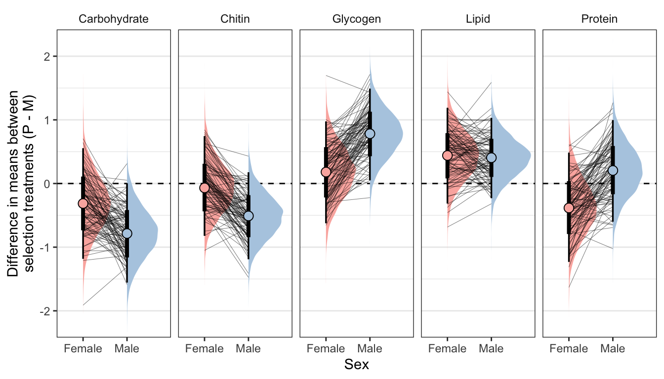

Version	Author	Date
43cc270	lukeholman	2020-12-09

Not controlling for differences in dry weight between sexes and treatments

treat_diff_actual_dryweight %>%
  filter(variable != 'Dryweight') %>% 
  ggplot(aes(x = sex, y = `Difference in means (Poly - Mono)`,fill = sex)) +
  geom_hline(yintercept = 0, linetype = 2) +
  stat_halfeye() + 
  geom_line(data = treat_diff_actual_dryweight %>%
              filter(draw %in% sampled_draws) %>%
              filter(variable != 'Dryweight'), 
            alpha = 0.8, size = 0.12, colour = "black", aes(group = draw)) +
  geom_point(data = summary_dat2, pch = 21, colour = "black", size = 3.1) + 
  scale_fill_brewer(palette = 'Pastel1', direction = 1, name = "") +
  scale_colour_brewer(palette = 'Pastel1', direction = 1, name = "") +
  facet_wrap( ~ variable,  nrow = 1) +
  theme_bw() +
  theme(legend.position = 'none',
        strip.background = element_blank(),
        panel.grid.major.x = element_blank()) +
  coord_cartesian(ylim = c(-1.8, 1.8)) + 
  ylab("Difference in means between\nselection treatments (P - M)") + xlab("Sex")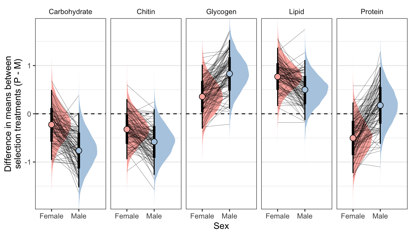

Version	Author	Date
43cc270	lukeholman	2020-12-09

Table

Controlling for differences in dry weight between sexes and treatments

summary_dat1 %>%
  kable(digits=3) %>%
  kable_styling(full_width = FALSE)

variable	sex	Difference in means (Poly - Mono)	Lower 95% CI	Upper 95% CI	p
Carbohydrate	Female	-0.314	-1.183	0.555	0.237
Carbohydrate	Male	-0.785	-1.556	0.004	0.025
Chitin	Female	-0.068	-0.822	0.745	0.435
Chitin	Male	-0.509	-1.190	0.177	0.069
Glycogen	Female	0.180	-0.625	0.976	0.335
Glycogen	Male	0.782	0.051	1.491	0.018
Lipid	Female	0.440	-0.314	1.189	0.122
Lipid	Male	0.405	-0.230	1.031	0.103
Protein	Female	-0.384	-1.232	0.484	0.191
Protein	Male	0.205	-0.600	0.997	0.304

Not controlling for differences in dry weight between sexes and treatments

summary_dat2 %>%
  kable(digits=3) %>%
  kable_styling(full_width = FALSE)

variable	sex	Difference in means (Poly - Mono)	Lower 95% CI	Upper 95% CI	p
Carbohydrate	Female	-0.225	-0.956	0.495	0.267
Carbohydrate	Male	-0.764	-1.526	0.018	0.027
Chitin	Female	-0.322	-0.943	0.305	0.158
Chitin	Male	-0.580	-1.264	0.095	0.044
Glycogen	Female	0.356	-0.307	1.019	0.146
Glycogen	Male	0.831	0.104	1.533	0.013
Lipid	Female	0.770	0.162	1.369	0.009
Lipid	Male	0.500	-0.130	1.115	0.058
Protein	Female	-0.502	-1.229	0.234	0.092
Protein	Male	0.175	-0.623	0.964	0.332

Posterior difference in treatment effect size between sexes

This section essentially examines the treatment \(\times\) sex interaction term, by calculating the difference in the effect size of the P/M treatment between sexes, for each of the five metabolites. We find no strong evidence for a treatment \(\times\) sex interaction, i.e. the treatment effects did not differ detectably between sexes. However, the effect of the Polyandry treatment on glycogen concentration appears to be marginally more positive in males than females (probability of direction = 92.5%, similar to a one-sided p-value of 0.075).

Figure

Controlling for differences in dry weight between sexes and treatments

treatsex_interaction_data1 <- treat_diff_standard_dryweight %>%
  select(draw, variable, sex, d =  `Difference in means (Poly - Mono)`) %>%
  arrange(draw, variable, sex) %>%
  group_by(draw, variable) %>%
  summarise(`Difference in effect size between sexes` = d[2] - d[1],
            .groups = "drop") # males - females


treatsex_interaction_data1 %>%
  filter(variable != 'Dryweight') %>% 
  ggplot(aes(x = `Difference in effect size between sexes`, y = 1, fill = stat(x < 0))) +
  geom_vline(xintercept = 0, linetype = 2) +
  stat_halfeyeh() +
  facet_wrap( ~ variable) +
  scale_fill_brewer(palette = 'Pastel2', direction = 1, name = "") +
  theme_bw() +
  theme(legend.position = 'none',
        strip.background = element_blank()) +
  ylab("Posterior density")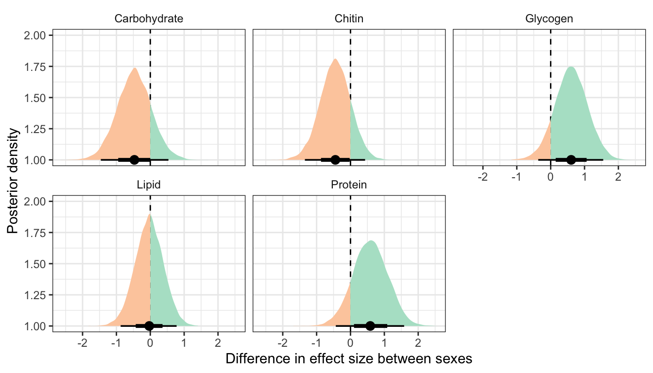

Version	Author	Date
43cc270	lukeholman	2020-12-09

Not controlling for differences in dry weight between sexes and treatments

treatsex_interaction_data2 <- treat_diff_actual_dryweight %>%
  select(draw, variable, sex, d =  `Difference in means (Poly - Mono)`) %>%
  arrange(draw, variable, sex) %>%
  group_by(draw, variable) %>%
  summarise(`Difference in effect size between sexes` = d[2] - d[1],
            .groups = "drop") # males - females


treatsex_interaction_data2 %>%
  filter(variable != 'Dryweight') %>% 
  ggplot(aes(x = `Difference in effect size between sexes`, y = 1, fill = stat(x < 0))) +
  geom_vline(xintercept = 0, linetype = 2) +
  stat_halfeyeh() +
  facet_wrap( ~ variable) +
  scale_fill_brewer(palette = 'Pastel2', direction = 1, name = "") +
  theme_bw() +
  theme(legend.position = 'none',
        strip.background = element_blank()) +
  ylab("Posterior density")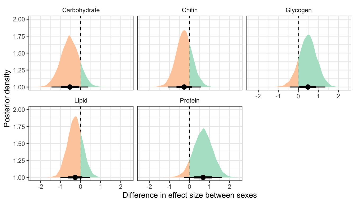

Version	Author	Date
43cc270	lukeholman	2020-12-09

Table

Controlling for differences in dry weight between sexes and treatments

treatsex_interaction_data1 %>%
  filter(variable != 'Dryweight') %>%
  rename(x = `Difference in effect size between sexes`) %>%
  group_by(variable)  %>%
  summarise(`Difference in effect size between sexes` = median(x),
            `Lower 95% CI` = quantile(x, probs = 0.025), 
            `Upper 95% CI` = quantile(x, probs = 0.975),
            p = 1 - as.numeric(bayestestR::p_direction(x)),
            ` ` = ifelse(p < 0.05, "*", ""),
            .groups = "drop") %>%
  kable(digits=3) %>%
  kable_styling(full_width = FALSE)

variable	Difference in effect size between sexes	Lower 95% CI	Upper 95% CI	p
Carbohydrate	-0.470	-1.461	0.536	0.170
Chitin	-0.446	-1.347	0.432	0.158
Glycogen	0.606	-0.367	1.552	0.105
Lipid	-0.031	-0.875	0.777	0.468
Protein	0.584	-0.434	1.584	0.126

Not controlling for differences in dry weight between sexes and treatments

treatsex_interaction_data2 %>%
  filter(variable != 'Dryweight') %>%
  rename(x = `Difference in effect size between sexes`) %>%
  group_by(variable)  %>%
  summarise(`Difference in effect size between sexes` = median(x),
            `Lower 95% CI` = quantile(x, probs = 0.025), 
            `Upper 95% CI` = quantile(x, probs = 0.975),
            p = 1 - as.numeric(bayestestR::p_direction(x)),
            ` ` = ifelse(p < 0.05, "*", ""),
            .groups = "drop") %>%
  kable(digits=3) %>%
  kable_styling(full_width = FALSE)

variable	Difference in effect size between sexes	Lower 95% CI	Upper 95% CI	p
Carbohydrate	-0.539	-1.454	0.380	0.124
Chitin	-0.265	-1.074	0.565	0.257
Glycogen	0.476	-0.429	1.350	0.142
Lipid	-0.275	-1.009	0.467	0.232
Protein	0.679	-0.276	1.606	0.081

sessionInfo()

R version 4.0.3 (2020-10-10)
Platform: x86_64-apple-darwin17.0 (64-bit)
Running under: macOS Catalina 10.15.4

Matrix products: default
BLAS:   /Library/Frameworks/R.framework/Versions/4.0/Resources/lib/libRblas.dylib
LAPACK: /Library/Frameworks/R.framework/Versions/4.0/Resources/lib/libRlapack.dylib

locale:
[1] en_AU.UTF-8/en_AU.UTF-8/en_AU.UTF-8/C/en_AU.UTF-8/en_AU.UTF-8

attached base packages:
[1] stats     graphics  grDevices utils     datasets  methods   base     

other attached packages:
 [1] knitrhooks_0.0.4 knitr_1.30       kableExtra_1.1.0 DT_0.13          tidybayes_2.0.3  brms_2.14.4      Rcpp_1.0.4.6     ggridges_0.5.2   gridExtra_2.3   
[10] GGally_1.5.0     forcats_0.5.0    stringr_1.4.0    dplyr_1.0.0      purrr_0.3.4      readr_1.3.1      tidyr_1.1.0      tibble_3.0.1     ggplot2_3.3.2   
[19] tidyverse_1.3.0  workflowr_1.6.2 

loaded via a namespace (and not attached):
  [1] readxl_1.3.1         backports_1.1.7      plyr_1.8.6           igraph_1.2.5         svUnit_1.0.3         splines_4.0.3        crosstalk_1.1.0.1   
  [8] TH.data_1.0-10       rstantools_2.1.1     inline_0.3.15        digest_0.6.25        htmltools_0.5.0      rsconnect_0.8.16     fansi_0.4.1         
 [15] magrittr_2.0.1       modelr_0.1.8         RcppParallel_5.0.1   matrixStats_0.56.0   xts_0.12-0           sandwich_2.5-1       prettyunits_1.1.1   
 [22] colorspace_1.4-1     blob_1.2.1           rvest_0.3.5          haven_2.3.1          xfun_0.19            callr_3.4.3          crayon_1.3.4        
 [29] jsonlite_1.7.0       lme4_1.1-23          survival_3.2-7       zoo_1.8-8            glue_1.4.2           gtable_0.3.0         emmeans_1.4.7       
 [36] webshot_0.5.2        V8_3.4.0             pkgbuild_1.0.8       rstan_2.21.2         abind_1.4-5          scales_1.1.1         mvtnorm_1.1-0       
 [43] DBI_1.1.0            miniUI_0.1.1.1       viridisLite_0.3.0    xtable_1.8-4         stats4_4.0.3         StanHeaders_2.21.0-3 htmlwidgets_1.5.1   
 [50] httr_1.4.1           DiagrammeR_1.0.6.1   threejs_0.3.3        arrayhelpers_1.1-0   RColorBrewer_1.1-2   ellipsis_0.3.1       farver_2.0.3        
 [57] pkgconfig_2.0.3      reshape_0.8.8        loo_2.3.1            dbplyr_1.4.4         labeling_0.3         tidyselect_1.1.0     rlang_0.4.6         
 [64] reshape2_1.4.4       later_1.0.0          visNetwork_2.0.9     munsell_0.5.0        cellranger_1.1.0     tools_4.0.3          cli_2.0.2           
 [71] generics_0.0.2       broom_0.5.6          evaluate_0.14        fastmap_1.0.1        yaml_2.2.1           processx_3.4.2       fs_1.4.1            
 [78] nlme_3.1-149         whisker_0.4          mime_0.9             projpred_2.0.2       xml2_1.3.2           compiler_4.0.3       bayesplot_1.7.2     
 [85] shinythemes_1.1.2    rstudioapi_0.11      gamm4_0.2-6          curl_4.3             reprex_0.3.0         statmod_1.4.34       stringi_1.5.3       
 [92] highr_0.8            ps_1.3.3             Brobdingnag_1.2-6    lattice_0.20-41      Matrix_1.2-18        nloptr_1.2.2.1       markdown_1.1        
 [99] shinyjs_1.1          vctrs_0.3.0          pillar_1.4.4         lifecycle_0.2.0      bridgesampling_1.0-0 estimability_1.3     insight_0.8.4       
[106] httpuv_1.5.3.1       R6_2.4.1             promises_1.1.0       codetools_0.2-16     boot_1.3-25          colourpicker_1.0     MASS_7.3-53         
[113] gtools_3.8.2         assertthat_0.2.1     rprojroot_1.3-2      withr_2.2.0          shinystan_2.5.0      multcomp_1.4-13      bayestestR_0.6.0    
[120] mgcv_1.8-33          parallel_4.0.3       hms_0.5.3            grid_4.0.3           coda_0.19-3          minqa_1.2.4          rmarkdown_2.5       
[127] git2r_0.27.1         shiny_1.4.0.2        lubridate_1.7.8      base64enc_0.1-3      dygraphs_1.1.1.6

Metabolic rates

Load packages

Load metabolite composition data

Inspect the raw data

Raw numbers

Simple plots

Plot of correlations between variables

Directed acyclic graph (DAG)

Fit brms structural equation model

Define Priors

Define the six sub-models

Running the model

Posterior predictive check of model fit

Table of model parameter estimates

Formatted table

Complete output from summary.brmsfit()

Posterior effect size of treatment on metabolite abundance, for each sex

Figure

Controlling for differences in dry weight between sexes and treatments

Not controlling for differences in dry weight between sexes and treatments

Table

Controlling for differences in dry weight between sexes and treatments

Not controlling for differences in dry weight between sexes and treatments

Posterior difference in treatment effect size between sexes

Figure

Controlling for differences in dry weight between sexes and treatments

Not controlling for differences in dry weight between sexes and treatments

Table

Controlling for differences in dry weight between sexes and treatments

Not controlling for differences in dry weight between sexes and treatments

Fit `brms` structural equation model

Complete output from `summary.brmsfit()`