Analysis of Experiment 3
Last updated: 2020-04-24
Checks: 6 1
Knit directory: social_immunity/
This reproducible R Markdown analysis was created with workflowr (version 1.6.0). The Checks tab describes the reproducibility checks that were applied when the results were created. The Past versions tab lists the development history.
The R Markdown file has unstaged changes. To know which version of the R Markdown file created these results, you’ll want to first commit it to the Git repo. If you’re still working on the analysis, you can ignore this warning. When you’re finished, you can run wflow_publish to commit the R Markdown file and build the HTML.
Great job! The global environment was empty. Objects defined in the global environment can affect the analysis in your R Markdown file in unknown ways. For reproduciblity it’s best to always run the code in an empty environment.
The command set.seed(20191017) was run prior to running the code in the R Markdown file. Setting a seed ensures that any results that rely on randomness, e.g. subsampling or permutations, are reproducible.
Great job! Recording the operating system, R version, and package versions is critical for reproducibility.
Nice! There were no cached chunks for this analysis, so you can be confident that you successfully produced the results during this run.
Great job! Using relative paths to the files within your workflowr project makes it easier to run your code on other machines.
These are the previous versions of the R Markdown and HTML files. If you’ve configured a remote Git repository (see ?wflow_git_remote), click on the hyperlinks in the table below to view them.
| File | Version | Author | Date | Message |
|---|---|---|---|---|
| html | 8c3b471 | lukeholman | 2020-04-21 | Build site. |
| Rmd | 1ce9e19 | lukeholman | 2020-04-21 | First commit 2020 |
| html | 1ce9e19 | lukeholman | 2020-04-21 | First commit 2020 |
| Rmd | aae65cf | lukeholman | 2019-10-17 | First commit |
| html | aae65cf | lukeholman | 2019-10-17 | First commit |
Load data and R packages
# All but 1 of these packages can be easily installed from CRAN.
# However it was harder to install the showtext package. On Mac, I did this:
# installed 'homebrew' using Terminal: ruby -e "$(curl -fsSL https://raw.githubusercontent.com/Homebrew/install/master/install)"
# installed 'libpng' using Terminal: brew install libpng
# installed 'showtext' in R using: devtools::install_github("yixuan/showtext")
library(showtext)

library(brms)
library(bayesplot)
library(tidyverse)
library(gridExtra)
library(kableExtra)
library(bayestestR)
library(cowplot)
library(tidybayes)
source("code/helper_functions.R")

# set up nice font for figure
nice_font <- "PT Serif"
font_add_google(name = nice_font, family = nice_font, regular.wt = 400, bold.wt = 700)
showtext_auto()

files <- c("data/data_collection_sheets/hiveA_touching.csv",
           "data/data_collection_sheets/hiveB_touching.csv",
           "data/data_collection_sheets/hiveC_touching.csv",
           "data/data_collection_sheets/hiveD_touching.csv")

experiment3 <- map(
  files,
  ~ read_csv(.x) %>%
    gather(minute, touching, -tube) %>%
    mutate(treatment = ifelse(substr(tube, 1, 1) %in% c("A", "B"), "AB", "CD"),
           minute = as.numeric(minute),
           touching = as.integer(touching),
           hive = gsub("hive", "", str_extract(.x, "hive[ABCD]")),
           tube = paste(hive, tube, sep = "_"))
  ) %>% bind_rows() %>%
  mutate(treatment = replace(treatment,
                             treatment == "AB" & hive %in% c("A", "B"),
                             "Ringers"),
         treatment = replace(treatment,
                             treatment == "AB" & hive %in% c("C", "D"),
                             "LPS"),
         treatment = replace(treatment,
                             treatment == "CD" & hive %in% c("A", "B"),
                             "LPS"),
         treatment = replace(treatment,
                             treatment == "CD" & hive %in% c("C", "D"),
                             "Ringers")) %>%
  mutate(hive = replace(hive, hive == "A", "Garden"),
         hive = replace(hive, hive == "B", "Skylab"),
         hive = replace(hive, hive == "C", "Arts"),
         hive = replace(hive, hive == "D", "Zoology"))


expt3_counts <- experiment3 %>%
  group_by(treatment, tube, hive) %>%
  summarise(n_touching = sum(touching),
            n_not_touching = sum(touching== 0),
            percent = n_touching / (n_touching + n_not_touching)) %>%
  ungroup() %>%
  filter(!is.na(n_touching)) %>%
  mutate(treatment = factor(treatment, c("Ringers", "LPS"))) %>%
  mutate(hive = C(factor(hive), sum)) # sum coding for hive
Inspect the raw data
Sample sizes by treatment
expt3_counts %>%
  group_by(treatment) %>%
  summarise(n = n()) %>%
kable() %>% kable_styling(full_width = FALSE)| treatment | n |
|---|---|
| Ringers | 220 |
| LPS | 219 |
Sample sizes by treatment and hive
expt3_counts %>%
  group_by(hive, treatment) %>%
  summarise(n = n()) %>%
kable() %>% kable_styling(full_width = FALSE)| hive | treatment | n |
|---|---|---|
| Arts | Ringers | 50 |
| Arts | LPS | 50 |
| Garden | Ringers | 70 |
| Garden | LPS | 70 |
| Skylab | Ringers | 50 |
| Skylab | LPS | 49 |
| Zoology | Ringers | 50 |
| Zoology | LPS | 50 |
Inspect the results
expt3_counts %>%
  group_by(hive, treatment) %>%
  summarise(pc = mean(100 * percent),
            SE = sd(percent) /sqrt(n()),
            n = n()) %>%
  rename(`% observations in which bees were in close contact` = pc,
         Hive = hive, Treatment = treatment) %>%
  kable(digits = 3) %>% kable_styling(full_width = FALSE) %>%
column_spec(3, width = "2in")| Hive | Treatment | % observations in which bees were in close contact | SE | n |
|---|---|---|---|---|
| Arts | Ringers | 69.509 | 0.036 | 50 |
| Arts | LPS | 72.547 | 0.033 | 50 |
| Garden | Ringers | 76.752 | 0.033 | 70 |
| Garden | LPS | 68.895 | 0.037 | 70 |
| Skylab | Ringers | 70.509 | 0.040 | 50 |
| Skylab | LPS | 65.653 | 0.034 | 49 |
| Zoology | Ringers | 84.075 | 0.021 | 50 |
| Zoology | LPS | 73.019 | 0.037 | 50 |
Plotted as a density histogram
Note that bees more often spent close to 100% of the observation period in contact in the control group, relative to the group treated with LPS.
raw_histogram <- expt3_counts %>%
  filter(treatment == "Ringers") %>%
  ggplot(aes(100 * percent,
             fill = treatment)) +
  geom_histogram(data = expt3_counts %>%
                   filter(treatment == "LPS"),
                 mapping = aes(y=..density..),
                 alpha = 0.5, bins = 11, colour = "black", linetype = 2) +
  geom_histogram(mapping = aes(y=..density..),
                 alpha = 0.5, bins = 11,
                 colour = "black") +
  scale_fill_brewer(palette = "Set1",
                    direction = 1, name = "Treatment") +
  xlab("% Time in close contact") + ylab("Density") +
  theme_bw() +
  theme(legend.position = c(0.27, 0.8),
        text = element_text(family = nice_font))

raw_histogram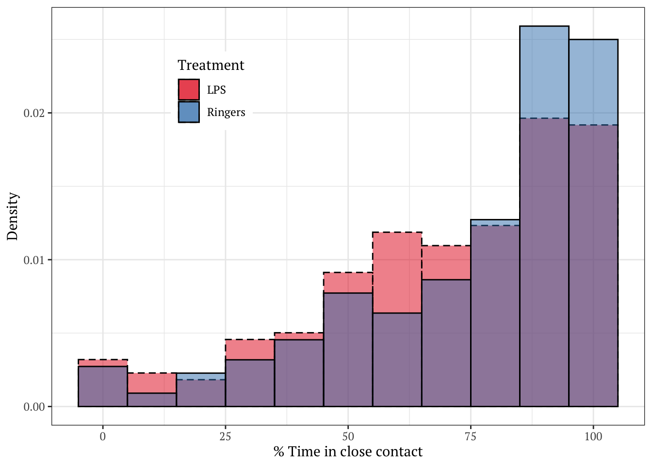
| Version | Author | Date |
|---|---|---|
| 1ce9e19 | lukeholman | 2020-04-21 |
Binomial model of time spent in contact
Run the models
Fit a binomial model, where the response is either a 0 (if bees were not in contact) or 1 (if they were). To assess the effects of our predictor variables, we compare 5 models with different fixed factors, ranking them by posterior model probability.
# new verison....
if(!file.exists("output/exp3_model.rds")){
  exp3_model_v1 <- brm(
    n_touching | trials(n) ~ treatment * hive + (1 | tube),
    data = expt3_counts %>% mutate(n = n_touching + n_not_touching),
    prior = c(set_prior("normal(0, 3)", class = "b")),
    family = "binomial", save_all_pars = TRUE, sample_prior = TRUE,
    chains = 4, cores = 1, iter = 20000, seed = 1)

  exp3_model_v2 <- brm(
    n_touching | trials(n) ~ treatment + hive + (1 | tube),
    data = expt3_counts %>% mutate(n = n_touching + n_not_touching),
    prior = c(set_prior("normal(0, 3)", class = "b")),
    family = "binomial", save_all_pars = TRUE, sample_prior = TRUE,
    chains = 4, cores = 1, iter = 20000, seed = 1)

  exp3_model_v3 <- brm(
    n_touching | trials(n) ~ hive + (1 | tube),
    data = expt3_counts %>% mutate(n = n_touching + n_not_touching),
    prior = c(set_prior("normal(0, 3)", class = "b")),
    family = "binomial",  save_all_pars = TRUE, sample_prior = TRUE,
    chains = 4, cores = 1, iter = 20000, seed = 1)

  posterior_model_probabilities <- tibble(
    Model = c("treatment * hive + observation_time_minutes",
              "treatment + hive + observation_time_minutes",
              "hive + observation_time_minutes"),
    post_prob = as.numeric(post_prob(exp3_model_v1,
                                     exp3_model_v2,
                                     exp3_model_v3))) %>%
    arrange(-post_prob)

  saveRDS(exp3_model_v2, "output/exp3_model.rds") # save the top model, treatment + hive
  saveRDS(posterior_model_probabilities, "output/exp3_post_prob.rds")
}
exp3_model <- readRDS("output/exp3_model.rds")
model_probabilities <- readRDS("output/exp3_post_prob.rds")
Posterior model probabilites
model_probabilities %>%
kable(digits = 3) %>% kable_styling(full_width = FALSE)| Model | post_prob |
|---|---|
| hive + observation_time_minutes | 0.720 |
| treatment + hive + observation_time_minutes | 0.278 |
| treatment * hive + observation_time_minutes | 0.001 |
Fixed effects from the top non-null model
tableS5 <- get_fixed_effects_with_p_values(exp3_model) %>%
  mutate(mu = map_chr(str_extract_all(Parameter, "mu[:digit:]"), ~ .x[1]),
         Parameter = str_remove_all(Parameter, "mu[:digit:]_"),
         Parameter = str_replace_all(Parameter, "treatment", "Treatment: "),
         Parameter = str_replace_all(Parameter, "observation_time_minutes", "Observation duration (minutes)")) %>%
  arrange(mu) %>%
  select(-mu, -Rhat, -Bulk_ESS, -Tail_ESS)

names(tableS5)[3:5] <- c("Est. Error", "Lower 95% CI", "Upper 95% CI")

saveRDS(tableS5, file = "figures/tableS5.rds")

tableS5 %>%
  kable(digits = 3) %>%
kable_styling(full_width = FALSE) | Parameter | Estimate | Est. Error | Lower 95% CI | Upper 95% CI | p | |
|---|---|---|---|---|---|---|
| Intercept | 1.678 | 0.141 | 1.401 | 1.960 | 0.000 | *** |
| Treatment: LPS | -0.369 | 0.199 | -0.763 | 0.022 | 0.033 | * |
| hive1 | -0.198 | 0.175 | -0.539 | 0.137 | 0.130 | |
| hive2 | 0.145 | 0.158 | -0.157 | 0.462 | 0.180 | |
| hive3 | -0.227 | 0.179 | -0.582 | 0.121 | 0.102 |
Table S5: Table summarising the posterior estimates of each fixed effect in the best-fitting model of Experiment 3 that contained the treatment effect. This was a binomial model where the response variable was 0 for observations in which bees were not in close contact, and 1 when they were. ‘Treatment’ is a fixed factor with two levels, and the effect of LPS shown here is expressed relative to the ‘Ringers’ treatment. ‘Hive’ was a fixed factor with four levels; unlike for treatment, we modelled hive using deviation coding, such that the intercept term represents the mean across all hives (in the Ringers treatment), and the three hive terms represent the deviation from this mean for three of the four hives. The model also included a random effect ‘pair ID’ (XXXXX), which grouped repeated observations made on each pair of bees, preventing pseudoreplication. The \(p\) column gives the posterior probability that the true effect size is opposite in sign to what is reported in the Estimate column, similarly to a p-value.
movement_files <- c("data/data_collection_sheets/hiveA_movement.csv",
                    "data/data_collection_sheets/hiveB_movement.csv",
                    "data/data_collection_sheets/hiveC_movement.csv",
                    "data/data_collection_sheets/hiveD_movement.csv")
movement <- map(1:4, ~ read_csv(movement_files[.x]) %>%
                  mutate(hive = c("A", "B", "C", "D")[.x]) %>%
                  gather(video, movement, -hive, -tube)) %>%
  bind_rows() %>%
  mutate(treatment = ifelse(substr(tube, 1, 1) %in% c("A", "B"), "AB", "CD")) %>%
  mutate(treatment = replace(treatment, treatment == "AB" & hive %in% c("A", "B"), "Ringers"),
         treatment = replace(treatment, treatment == "AB" & hive %in% c("C", "D"), "LPS"),
         treatment = replace(treatment, treatment == "CD" & hive %in% c("A", "B"), "LPS"),
         treatment = replace(treatment, treatment == "CD" & hive %in% c("C", "D"), "Ringers")) %>%
  split(.$hive) %>%
  map(~ .x %>% arrange(video) %>%
        mutate(video = as.numeric(factor(video, unique(video))))) %>%
  bind_rows() %>%
  mutate(hive = replace(hive, hive == "A", "Garden"),
         hive = replace(hive, hive == "B", "Skylab"),
         hive = replace(hive, hive == "C", "Arts"),
         hive = replace(hive, hive == "D", "Zoology"))

movement %>%
  mutate(movement = factor(movement)) %>%
  group_by(movement, treatment) %>%
  summarise(n=n()) %>%
  ggplot(aes(movement, n, fill = treatment)) +
  geom_bar(stat = "identity", colour = "grey20", position = "dodge") +
  scale_fill_brewer(palette="Pastel2", direction = 1)

library(brms)
mod <- brm(movement | cat(3) ~ treatment + (1 | tube),
           data = movement %>% mutate(movement = movement + 1), family = cumulative())
marginal_effects(mod, categorical = T)

new <- expand.grid(hive = c("Arts", "Garden", "Skylab", "Zoology"),
                   treatment = c("Ringers", "LPS"))

data.frame(new, rbind(fitted(mod, newdata = new, re_formula = NA)[,,1],
                      fitted(mod, newdata = new, re_formula = NA)[,,2],
                      fitted(mod, newdata = new, re_formula = NA)[,,3])) %>%
  mutate(movement = factor(rep(0:2, each = nrow(new)))) %>%
  ggplot(aes(movement, Estimate, ymin = Q2.5, ymax=Q97.5, colour = treatment)) +
  geom_errorbar(position = position_dodge(0.2), width = 0) +
  geom_point(position = position_dodge(0.2)) +
  facet_wrap(~ hive)
Plotting estimates from the model
# new test...
new <- expt3_counts %>%
  select(treatment) %>% distinct() %>%
  mutate(n = 100, key = paste("V", 1:n(), sep = ""),
         hive = NA)
plotting_data <- as.data.frame(fitted(exp3_model,
                                      newdata=new, re_formula = NA, summary = FALSE))
names(plotting_data) <- c("LPS", "Ringers")
plotting_data <- plotting_data %>% gather(treatment, percent_time_in_contact)

cols <- c("#34558b", "#4ec5a5", "#ffaf12")

dot_plot <- plotting_data %>%
  mutate(treatment = factor(treatment, c("Ringers", "LPS"))) %>%
  ggplot(aes(percent_time_in_contact, treatment)) +
  stat_dotsh(quantiles = 100, fill = "grey40", colour = "grey40") +
  stat_pointintervalh(
    mapping = aes(colour = treatment, fill = treatment),
    .width = c(0.5, 0.95),
    position = position_nudge(y = -0.07),
    point_colour = "grey26", pch = 21, stroke = 0.4) +
  xlab("Mean % time in close contact") + ylab("Treatment") +
  scale_colour_brewer(palette = "Pastel1",
                      direction = -1, name = "Treatment") +
  scale_fill_brewer(palette = "Pastel1",
                      direction = -1, name = "Treatment") +
  theme_bw() +
  coord_cartesian(ylim=c(1.4, 2.4)) +
  theme(
    text = element_text(family = nice_font),
    strip.background = element_rect(fill = "#eff0f1"),
    panel.grid.major.y = element_blank(),
    legend.position = "none"
  )

# positive effect = odds of this outcome are higher for trt2 than trt1 (put control as trt1)
get_log_odds <- function(trt1, trt2){
  log((trt2 / (1 - trt2) / (trt1 / (1 - trt1))))
}

LOR <- plotting_data %>%
  mutate(posterior_sample = rep(1:(n()/2), 2)) %>%
  spread(treatment, percent_time_in_contact) %>%
  mutate(LOR = get_log_odds(Ringers/100, LPS/100)) %>%
  select(LOR)

LOR_plot <- LOR %>%
  ggplot(aes(LOR, y =1)) +
  geom_vline(xintercept = 0, linetype = 2) +
  stat_dotsh(quantiles = 100, fill = "grey40", colour = "grey40") +
  stat_pointintervalh(
    colour = "orange", fill = "orange",
    .width = c(0.5, 0.95),
    position = position_nudge(y = -0.1),
    point_colour = "grey26", pch = 21, stroke = 0.4) +
  coord_cartesian(ylim=c(0.86, 2)) +
  xlab("Effect of LPS on % time\nin close contact (LOR)") +
  ylab("Posterior density") +
  theme_bw() +
  theme(
    text = element_text(family = nice_font),
    axis.text.y = element_blank(),
    axis.ticks.y = element_blank(),
    panel.grid.major.y = element_blank(),
    panel.grid.minor.y = element_blank(),
    legend.position = "none"
  )

p <- cowplot::plot_grid(raw_histogram,
                        dot_plot, LOR_plot,  labels = c("A", "B", "C"),
                        nrow = 1, align = 'h', axis = 'l')
ggsave(plot = p, filename = "figures/fig3.pdf", height = 3.2, width = 8.6)
p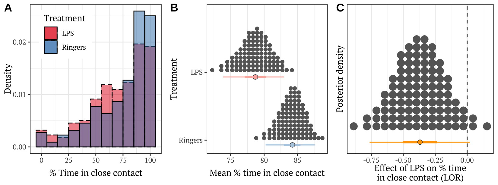
| Version | Author | Date |
|---|---|---|
| 1ce9e19 | lukeholman | 2020-04-21 |
Figure 3: Panel A shows the frequency distribution of the % time in close contact, for pairs of bees from the LPS treatment and the Ringers control. Panel B shows the posterior estimates of the mean % time spent in close contact; the details of the quantile dot plot and error bars are the same as described for Figure 1. Panel C shows the effect size (LOR; log odds ratio) associated with the difference in means in Panel B.
Hypothesis testing and effect sizes
get_log_odds <- function(trt1, trt2){
  log((trt2 / (1 - trt2) / (trt1 / (1 - trt1))))
}

my_summary <- function(df) {

  diff <- (df %>% pull(Ringers)) - (df %>% pull(LPS))
  LOR <- get_log_odds((df %>% pull(Ringers))/100,
                      (df %>% pull(LPS))/100)
  p <- 1 - (diff %>% bayestestR::p_direction() %>% as.numeric())
  diff <- diff %>% posterior_summary() %>% as_tibble()
  LOR <- LOR %>% posterior_summary() %>% as_tibble()
  output <- rbind(diff, LOR) %>%
    mutate(p=p,
           Metric = c("Absolute difference in % time in close contact",
                      "Log odds ratio")) %>%
      select(Metric, everything()) %>%
    mutate(p = format(round(p, 4), nsmall = 4))
  output$p[1] <- " "
  output
}

plotting_data %>%
  as_tibble() %>%
  mutate(sample = rep(1:(n() / 2), 2)) %>%
  spread(treatment, percent_time_in_contact) %>%
  mutate(difference = LPS - Ringers) %>%
  my_summary() %>%
  mutate(` ` = ifelse(p < 0.05, "\\*", ""),
         ` ` = replace(` `, p < 0.01, "**"),
         ` ` = replace(` `, p < 0.001, "***"),
         ` ` = replace(` `, p == " ", "")) %>%
kable(digits = 3) %>% kable_styling() | Metric | Estimate | Est.Error | Q2.5 | Q97.5 | p | |
|---|---|---|---|---|---|---|
| Absolute difference in % time in close contact | 5.538 | 3.006 | -0.330 | 11.495 | ||
| Log odds ratio | -0.369 | 0.199 | -0.763 | 0.022 | 0.0328 | * |
Table S6: Pairs in which one bee had received LPS were observed in close contact less frequently than pairs in which one bee had received Ringers solution.
sessionInfo()R version 3.6.3 (2020-02-29)
Platform: x86_64-apple-darwin15.6.0 (64-bit)
Running under: macOS Catalina 10.15.4
Matrix products: default
BLAS: /Library/Frameworks/R.framework/Versions/3.6/Resources/lib/libRblas.0.dylib
LAPACK: /Library/Frameworks/R.framework/Versions/3.6/Resources/lib/libRlapack.dylib
locale:
[1] en_AU.UTF-8/en_AU.UTF-8/en_AU.UTF-8/C/en_AU.UTF-8/en_AU.UTF-8
attached base packages:
[1] stats graphics grDevices utils datasets methods base
other attached packages:
[1] tidybayes_2.0.1 cowplot_1.0.0 bayestestR_0.5.1 kableExtra_1.1.0
[5] gridExtra_2.3 forcats_0.5.0 stringr_1.4.0 dplyr_0.8.5
[9] purrr_0.3.3 readr_1.3.1 tidyr_1.0.2 tibble_3.0.0
[13] ggplot2_3.3.0 tidyverse_1.3.0 bayesplot_1.7.1 brms_2.12.0
[17] Rcpp_1.0.3 showtext_0.7-1 showtextdb_2.0 sysfonts_0.8
loaded via a namespace (and not attached):
[1] colorspace_1.4-1 ellipsis_0.3.0 ggridges_0.5.2
[4] rsconnect_0.8.16 rprojroot_1.3-2 markdown_1.1
[7] base64enc_0.1-3 fs_1.3.1 rstudioapi_0.11
[10] farver_2.0.3 rstan_2.19.3 svUnit_0.7-12
[13] DT_0.13 fansi_0.4.1 mvtnorm_1.1-0
[16] lubridate_1.7.8 xml2_1.3.1 bridgesampling_1.0-0
[19] knitr_1.28 shinythemes_1.1.2 jsonlite_1.6.1
[22] workflowr_1.6.0 broom_0.5.4 dbplyr_1.4.2
[25] shiny_1.4.0 compiler_3.6.3 httr_1.4.1
[28] backports_1.1.6 assertthat_0.2.1 Matrix_1.2-18
[31] fastmap_1.0.1 cli_2.0.2 later_1.0.0
[34] htmltools_0.4.0 prettyunits_1.1.1 tools_3.6.3
[37] igraph_1.2.5 coda_0.19-3 gtable_0.3.0
[40] glue_1.4.0 reshape2_1.4.4 cellranger_1.1.0
[43] vctrs_0.2.4 nlme_3.1-147 crosstalk_1.1.0.1
[46] insight_0.8.1 xfun_0.13 ps_1.3.0
[49] rvest_0.3.5 mime_0.9 miniUI_0.1.1.1
[52] lifecycle_0.2.0 gtools_3.8.2 zoo_1.8-7
[55] scales_1.1.0 colourpicker_1.0 hms_0.5.3
[58] promises_1.1.0 Brobdingnag_1.2-6 parallel_3.6.3
[61] inline_0.3.15 RColorBrewer_1.1-2 shinystan_2.5.0
[64] curl_4.3 yaml_2.2.1 loo_2.2.0
[67] StanHeaders_2.19.2 stringi_1.4.6 highr_0.8
[70] dygraphs_1.1.1.6 pkgbuild_1.0.6 rlang_0.4.5
[73] pkgconfig_2.0.3 matrixStats_0.56.0 evaluate_0.14
[76] lattice_0.20-41 labeling_0.3 rstantools_2.0.0
[79] htmlwidgets_1.5.1 processx_3.4.2 tidyselect_1.0.0
[82] plyr_1.8.6 magrittr_1.5 R6_2.4.1
[85] generics_0.0.2 DBI_1.1.0 pillar_1.4.3
[88] haven_2.2.0 whisker_0.4 withr_2.1.2
[91] xts_0.12-0 abind_1.4-5 modelr_0.1.5
[94] crayon_1.3.4 arrayhelpers_1.1-0 rmarkdown_2.1
[97] grid_3.6.3 readxl_1.3.1 callr_3.4.3
[100] git2r_0.26.1 threejs_0.3.3 reprex_0.3.0
[103] digest_0.6.25 webshot_0.5.2 xtable_1.8-4
[106] httpuv_1.5.2 stats4_3.6.3 munsell_0.5.0
[109] viridisLite_0.3.0 shinyjs_1.1