datatable(joined_pretty_tot,
          rownames = FALSE,
          colnames = c("Meter status","Buildings", "Square\nfootage", "kWh", "Est. cost",
                       "CO2e\n(MT)",  "kWh per\nsqft"),
          filter = "none",
          class = "compact",
          options = list(pageLength = 4, autoWidth = TRUE, dom = 't'),
          caption = "Table 1. Totals for annual electricity use by meter type. Annual estimates for each meter were adjusted to account for missing days of electricity data.")
Individually metered buildings
datatable(joined_pretty_cat,
          rownames = FALSE,
          colnames = c("Building\ntype","Buildings\nwith data", "Median\nsquare\nfootage", "kWh",
                       "Est. cost", "CO2e\n(MT)", "Median\nkWh\nper sqft",
                       "25th Perc.", "75th Perc."),
          filter = "none",
          class = "compact",
          options = list(pageLength = 11, autoWidth = TRUE, dom = 't'),
          caption = "Table 2. Descriptive statistics for annual electricity use by building type for buildings with individual electricity use data. Annual estimates for each meter were adjusted to account for missing days of electricity data.")
Electricity use over the year
daily_graph <- daily_full %>%
mutate(date = as_date(date),
month = month(date, label = TRUE),
day = wday(date, label = TRUE),
type_brief = recode(type,
'Res Hall - U' = 'Residential',
'Res Hall - S' = 'Residential',
'Res Hall - M' = 'Residential',
'Res Hall - L' = 'Residential')) %>%
filter(!is.na(month))
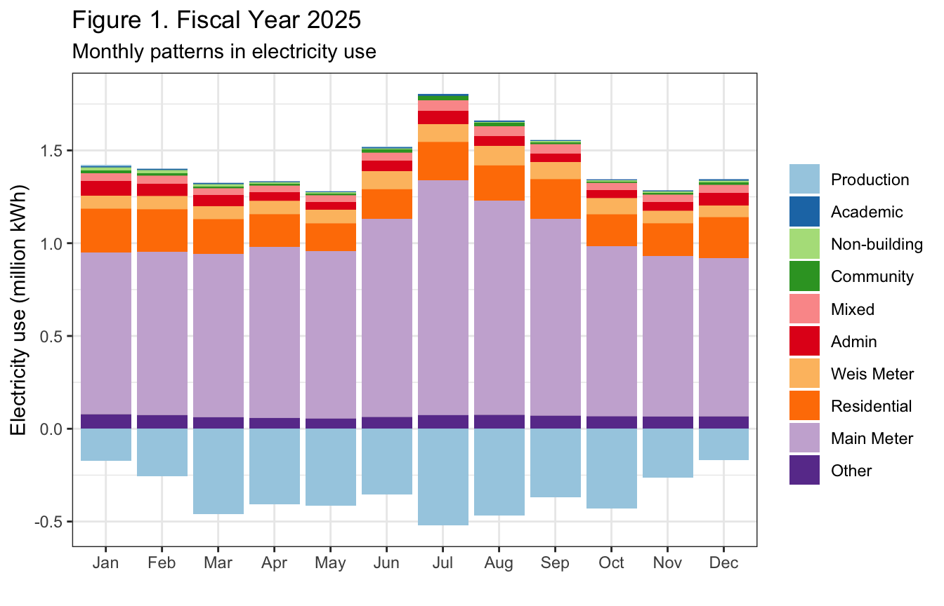
ggplot(filter(daily_graph, meter != "Submeter"),
aes(x = month, y = kwh/10^6, fill = reorder(type_brief, kwh, FUN = sum))) +
geom_col(position = "stack") +
scale_fill_brewer(type = "qual", palette = "Paired") +
theme_bw() +
labs(x = "", y = "Electricity use (million kWh)", fill = "",
title = "Figure 1. Fiscal Year 2025",
subtitle = "Monthly patterns in electricity use")
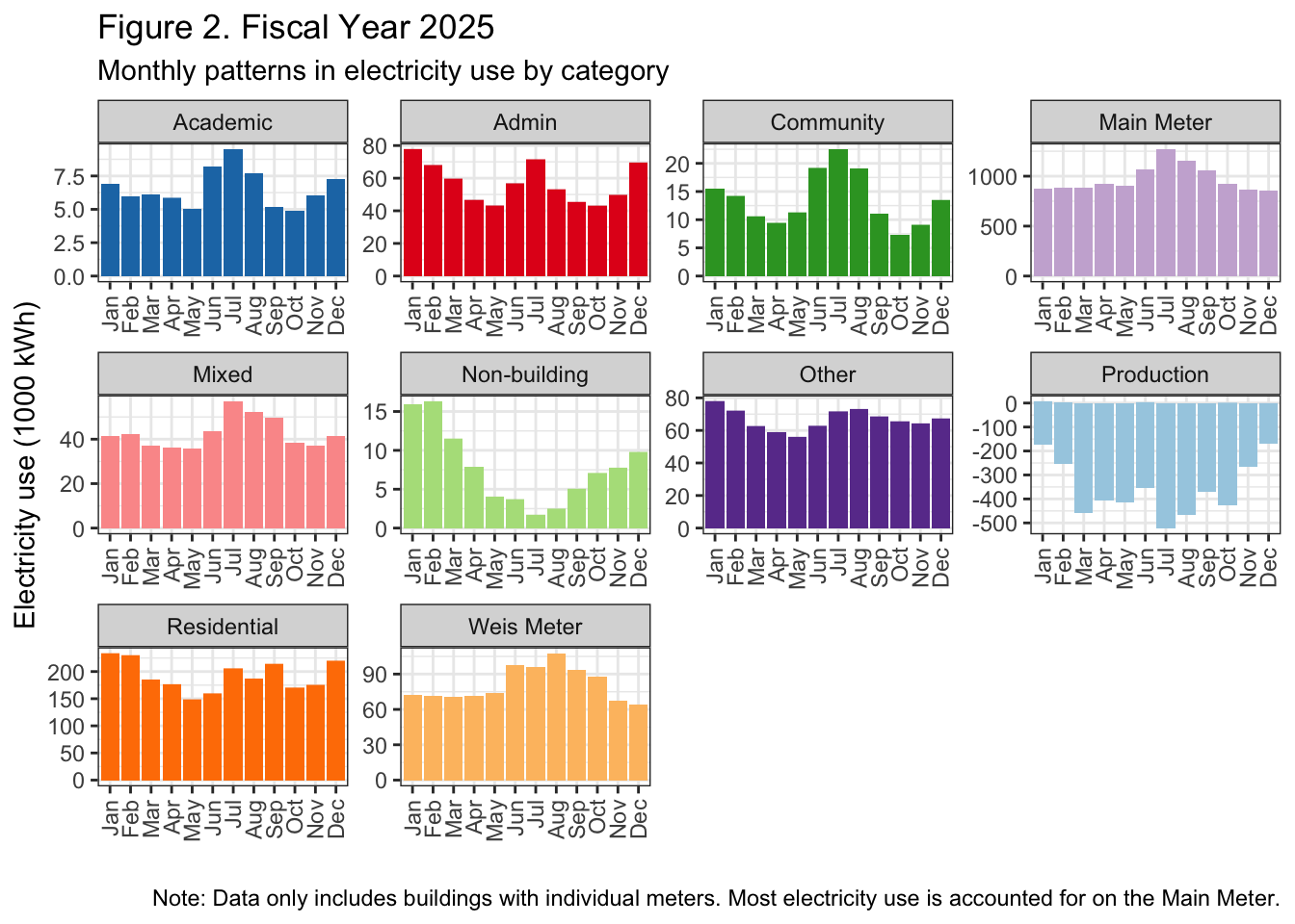
ggplot(filter(daily_graph, meter != "Submeter"),
       aes(x = month, y = kwh/10^3, fill = reorder(type_brief, kwh, FUN = sum))) +
  geom_col(position = "stack") +
  facet_wrap(. ~ type_brief, scales = "free") +
  scale_fill_brewer(type = "qual", palette = "Paired") +
  theme_bw() +
  theme(legend.position = "none") +
  theme(axis.text.x = element_text(angle = 90, vjust = 0.5, hjust = 1)) +
  labs(x = "", y = "Electricity use (1000 kWh)", fill = "",
       title = "Figure 2. Fiscal Year 2025",
       subtitle = "Monthly patterns in electricity use by category",
       caption = "Note: Data only includes buildings with individual meters. Most electricity use is accounted for on the Main Meter.")
Electricity intensity
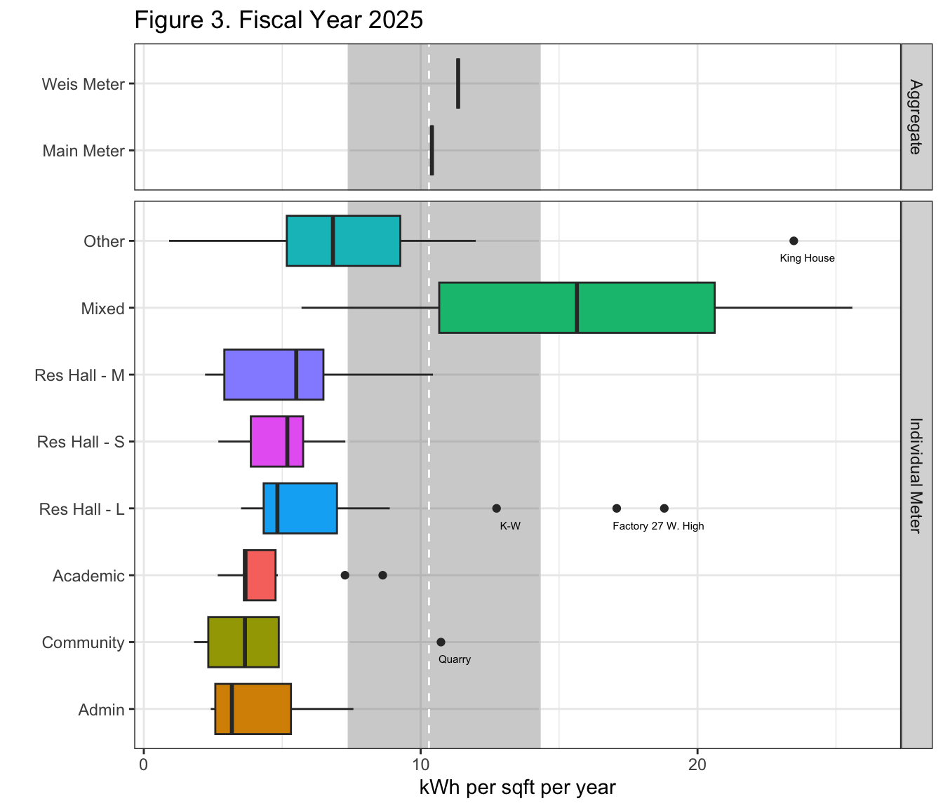
intensity <- joined_full %>%
  filter(!(type %in% c("Res Hall - U","Production", "Non-building"))) %>%
  mutate(kwh_sqft = kwh_corr/sqft,
         meter_type = ifelse(type %in% c("Main Meter","Weis Meter"), "Aggregate", "Individual Meter"),
         outlier = case_when(
           NAME == "King House" ~ "King House",
           NAME == "Kisner - Woodward" ~ "K-W",
           NAME == "Factory Apts." ~ "Factory",
           NAME == "Rector Science Center" ~ "Rector",
           NAME == "Quarry, The " ~ "Quarry",
           NAME == "27 W. High St." ~ "27 W. High"
         ))

# median and IQR come from EIA (2022) table, annual kWh per square foot for Colleges/Universities
# https://www.eia.gov/consumption/commercial/data/2018/ce/pdf/c22.pdf

ggplot(intensity,
       aes(x = reorder(type, kwh_sqft, FUN = "median"),
                        y = kwh_sqft, fill = type)) +
  annotate("rect", xmin = -Inf, xmax = Inf, ymin = 7.4, ymax = 14.3, color = "lightgray", alpha = 0.3) +
  geom_hline(yintercept = 10.3, linetype = "dashed", color = "white") +
  facet_grid(meter_type ~ ., scales = "free_y", space = "free_y") +
  geom_boxplot() +
  geom_label(aes(label = outlier), na.rm = TRUE, nudge_x = -0.25, nudge_y = 0.5,
             color = "black", fill = "white", size = 2, alpha = 0, label.size = NA) +
  coord_flip() +
  theme_bw() +
  theme(legend.position = "none") +
  labs(x = "", y = "kWh per sqft per year",
       title = "Figure 3. Fiscal Year 2025")