Campus building summary
Maggie Douglas
03/07/26
Load data
library(tidyverse)
library(DT) # library to create tables
library(scales) # library to format dollars
library(RColorBrewer)

is_outlier <- function(x) {
  return(x < quantile(x, 0.25, na.rm = T) - 1.5 * IQR(x, na.rm = T) | x > quantile(x, 0.75, na.rm = T) + 1.5 * IQR(x, na.rm = T))
}
daily_full <- read.csv("./output/kwh_daily_2026-03-04.csv") %>%
mutate(date = as_date(date)) # convert back to date
joined_full <- read.csv("./output/kwh_annual_2026-03-04.csv")
total <- joined_full %>%
filter(meter != "Submeter" & type != "Res Hall - U" & type != "Production") %>%
summarize(kwh = sum(kwh, na.rm = T),
kwh_corr = sum(kwh_corr, na.rm = T),
sqft = sum(sqft, na.rm = T)) %>%
mutate(kwh_sqft = kwh_corr/sqft,
meter = "Total")
buildings <- read.csv("./keys/fy25_building_list_updated.csv") %>%
mutate(meter = ifelse(weis_meter == 1, "Weis Meter",
ifelse(main_meter == 0 & weis_meter == 0, "Individually Metered", "Main Meter")))
# store conversion factors
dollars_kwh <- 0.08138507
co2_kg_kwh <- 0.30082405# summarize # buildings by meter status
bldg_sum <- buildings %>%
group_by(meter) %>%
summarize(number = n())
bldg_tot <- bldg_sum %>%
summarize(number = sum(number)) %>%
mutate(meter = "Total")
bldg_comb <- rbind(bldg_sum, bldg_tot)
# generate summary for Main, Weis, and Individual meters
joined_agg <- joined_full %>%
ungroup() %>%
filter(meter != "Submeter" & type != "Res Hall - U" & type != "Production") %>%
group_by(meter) %>%
summarize(kwh = sum(kwh, na.rm = T),
kwh_corr = sum(kwh_corr, na.rm = T),
sqft = sum(sqft, na.rm = T)) %>%
mutate(kwh_sqft = kwh_corr/sqft) %>%
rbind(total) %>%
mutate(dollars = kwh_corr*dollars_kwh,
ghg_MTCO2 = (kwh_corr*co2_kg_kwh)/1000) %>%
select(-kwh) %>%
arrange(kwh_corr)
joined_agg$meter <- factor(joined_agg$meter,
levels = c("Main Meter - Total",
"Weis Meter - Total",
"Individual", "Total"),
labels = c("Main Meter", "Weis Meter",
"Individually Metered","Total"))
joined_tot <- joined_agg %>%
left_join(bldg_comb, by = "meter")# generate summary by building category for individually metered buildings
joined_cat <- joined_full %>%
filter(meter %in% c("Individual","Submeter")) %>%
mutate(kwh_sqft = kwh_corr/sqft, # calculate kwh per sqft
kwh_person = kwh_corr/occupants,
dollars = kwh_corr*dollars_kwh,
ghg_kgCO2 = kwh_corr*co2_kg_kwh) %>%
group_by(type) %>%
summarize(n = n(),
kwh = sum(kwh_corr),
dollars = sum(dollars),
ghg_kgCO2 = sum(ghg_kgCO2),
sqft = median(sqft, na.rm = T),
med_kwh_sqft = median(kwh_sqft, na.rm = T),
kwh_sqft_25 = quantile(kwh_sqft, .25, na.rm = T),
kwh_sqft_75 = quantile(kwh_sqft, .75, na.rm = T)) %>%
arrange(-kwh)Electricity use summary
joined_pretty_tot <- joined_tot %>%
  mutate(kwh = round(kwh_corr, digits = 0),
         dollars = paste("$",round(dollars, digits = 0)),
         ghg_MTCO2 = round(ghg_MTCO2, digits = 0),
         sqft = round(sqft, digits = 0),
         kwh_sqft = round(kwh_sqft, digits = 1)) %>%
  select(meter, number, sqft, kwh, dollars, ghg_MTCO2, kwh_sqft) %>%
  arrange(kwh)

joined_pretty_cat <- joined_cat %>%
  mutate(kwh = round(kwh, digits = 0),
         dollars = paste("$",round(dollars, digits = 0)),
         ghg_MTCO2 = round(ghg_kgCO2/1000, digits = 0),
         sqft = round(sqft, digits = 0),
         med_kwh_sqft = round(med_kwh_sqft, digits = 1),
         kwh_sqft_25 = round(kwh_sqft_25, digits = 1),
         kwh_sqft_75 = round(kwh_sqft_75, digits = 1)) %>%
    select(type, n, sqft, kwh, dollars, ghg_MTCO2, med_kwh_sqft, kwh_sqft_25, kwh_sqft_75) %>%
  arrange(desc(med_kwh_sqft))
Aggregate meters
datatable(joined_pretty_tot,
          rownames = FALSE,
          colnames = c("Meter status","Buildings", "Square\nfootage", "kWh", "Est. cost",
                       "CO2e\n(MT)",  "kWh per\nsqft"),
          filter = "none",
          class = "compact",
          options = list(pageLength = 4, autoWidth = TRUE, dom = 't'),
          caption = "Table 1. Totals for annual electricity use by meter type. Annual estimates for each meter were adjusted to account for missing days of electricity data.")
Individually metered buildings
datatable(joined_pretty_cat,
          rownames = FALSE,
          colnames = c("Building\ntype","Buildings\nwith data", "Median\nsquare\nfootage", "kWh",
                       "Est. cost", "CO2e\n(MT)", "Median\nkWh\nper sqft",
                       "25th Perc.", "75th Perc."),
          filter = "none",
          class = "compact",
          options = list(pageLength = 11, autoWidth = TRUE, dom = 't'),
          caption = "Table 2. Descriptive statistics for annual electricity use by building type for buildings with individual electricity use data. Annual estimates for each meter were adjusted to account for missing days of electricity data.")
Electricity use over the year
Total
daily_graph <- daily_full %>%
  mutate(date = as_date(date),
         month = month(date, label = TRUE),
         day = wday(date, label = TRUE),
         type_brief = recode(type,
                       'Res Hall - U' = 'Res Hall',
                       'Res Hall - S' = 'Res Hall',
                       'Res Hall - M' = 'Res Hall',
                       'Res Hall - L' = 'Res Hall')) %>%
  filter(!is.na(month))

ggplot(filter(daily_graph, meter != "Submeter"),
       aes(x = month, y = kwh/10^6, fill = reorder(type_brief, kwh, FUN = sum))) +
  geom_col(position = "stack") +
  scale_fill_brewer(type = "qual", palette = "Paired") +
  theme_bw() +
  labs(x = "", y = "Electricity use (million kWh)", fill = "",
       title = "")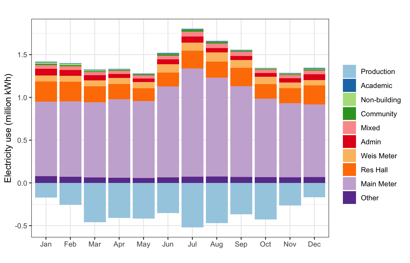
| Version | Author | Date |
|---|---|---|
| 92fcd5c | maggiedouglas | 2026-03-04 |
Submeter data
ggplot(filter(daily_graph, meter == "Submeter"),
       aes(x = month, y = kwh/10^6, fill = reorder(type_brief, kwh, FUN = sum))) +
  geom_col(position = "stack") +
  scale_fill_brewer(type = "qual", palette = "Paired") +
  theme_bw() +
  labs(x = "", y = "Electricity use (million kWh)", fill = "",
       title = "")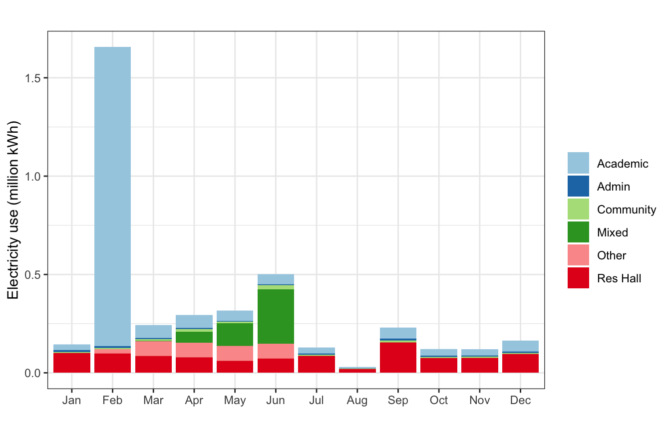
| Version | Author | Date |
|---|---|---|
| 92fcd5c | maggiedouglas | 2026-03-04 |
Aggregate meters
Here’s an example where the Y axis is fixed
daily_graph$meter2 <- factor(daily_graph$meter,
                            levels = c("Main Meter - Total","Weis Meter - Total",
                                       "Individual","Submeter"),
                            labels = c("Aggregate","Aggregate", "Individual","Submeter"))

ggplot(filter(daily_graph, meter2 == "Aggregate"),
       aes(x = month, y = kwh/10^3, fill = reorder(type, kwh, FUN = 'sum'))) +
  geom_col(position = "stack") +
  facet_wrap(. ~ type) +
  theme_bw() +
  labs(x = "", y = "Electricity use (1000 kWh)", fill = "") +
  theme(axis.text.x = element_text(angle = 90, hjust = 1, vjust = 0.5)) +
  theme(legend.position = "none")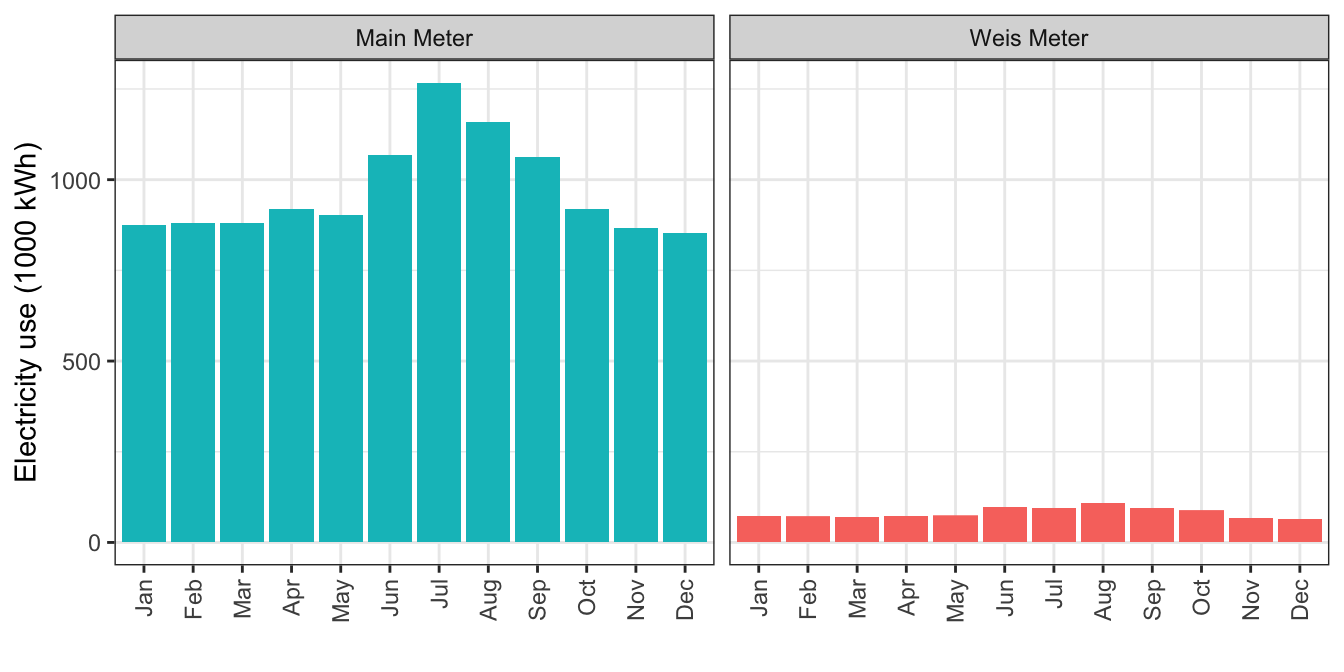
Individual meters
Here’s an example where the Y axis is allowed to vary
ggplot(filter(daily_graph, meter == "Individual"),
       aes(x = month, y = kwh/10^3, fill = reorder(type, kwh, FUN = 'sum'))) +
  geom_col(position = "stack") +
  facet_wrap(. ~ type, scales = "free") +
  theme_bw() +
  labs(x = "", y = "Electricity use (1000 kWh)", fill = "") +
  theme(axis.text.x = element_text(angle = 90, hjust = 1, vjust = 0.5)) +
  theme(legend.position = "none")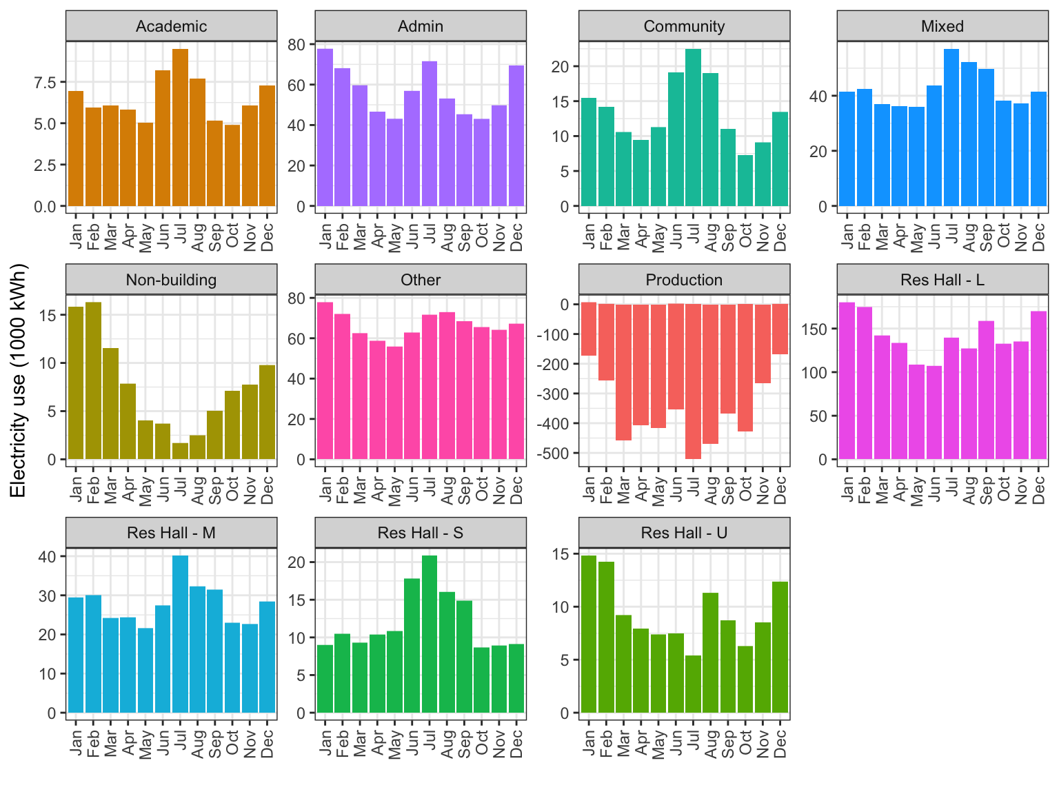
Submeters
ggplot(filter(daily_graph, meter == "Submeter"),
       aes(x = month, y = kwh/10^3, fill = reorder(type, kwh, FUN = 'sum'))) +
  geom_col(position = "stack") +
  facet_wrap(. ~ type, scales = "free") +
  theme_bw() +
  labs(x = "", y = "Electricity use (1000 kWh)", fill = "") +
  theme(axis.text.x = element_text(angle = 90, hjust = 1, vjust = 0.5)) +
  theme(legend.position = "none")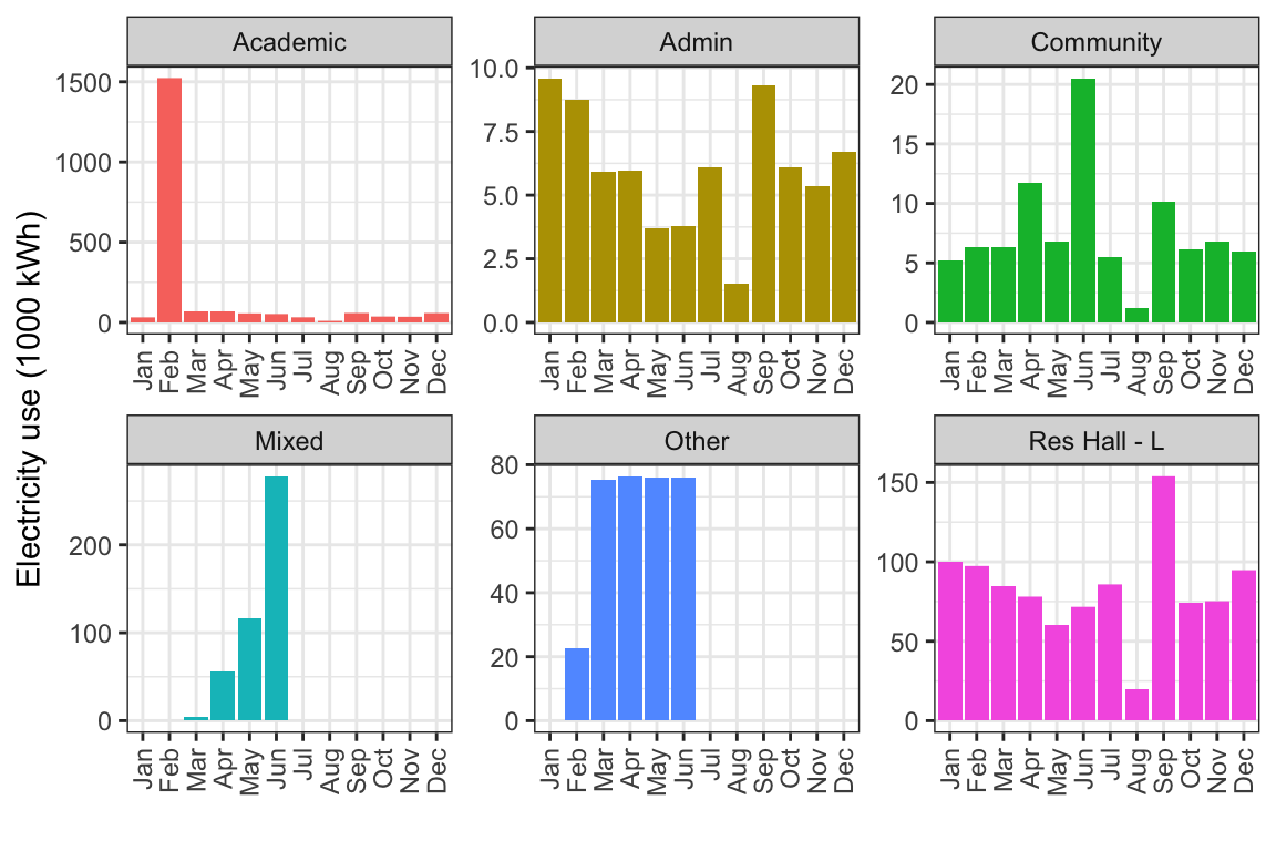
Electricity intensity by building type
to_exclude <- filter(joined_full, days_perc < 90)

intensity <- joined_full %>%
  filter(!(type %in% c("Res Hall - U","Production", "Non-building"))) %>%
  mutate(kwh_sqft = kwh_corr/sqft,
         meter_type = ifelse(type %in% c("Main Meter","Weis Meter"), "Aggregate", "Individual Meter"),
         outlier = case_when(
           NAME == "King House" ~ "King House",
           NAME == "Kisner - Woodward" ~ "K-W",
           NAME == "Factory Apts." ~ "Factory",
           NAME == "Rector Science Center" ~ "Rector",
           NAME == "Quarry, The " ~ "Quarry",
           NAME == "27 W. High St." ~ "27 W. High"
         ))


# median and IQR come from EIA (2022) table, annual kWh per square foot for Colleges/Universities
# https://www.eia.gov/consumption/commercial/data/2018/ce/pdf/c22.pdf

ggplot(intensity,
       aes(x = reorder(type, kwh_sqft, FUN = "median"),
                        y = kwh_sqft, fill = type)) +
  annotate("rect", xmin = -Inf, xmax = Inf, ymin = 7.4, ymax = 14.3, color = "lightgray", alpha = 0.3) +
  geom_hline(yintercept = 10.3, linetype = "dashed", color = "white") +
  facet_grid(meter_type ~ ., scales = "free_y", space = "free_y") +
  geom_boxplot() +
  geom_label(aes(label = outlier), na.rm = TRUE, nudge_x = -0.25, nudge_y = 0.5,
             color = "black", fill = "white", size = 2, alpha = 0, label.size = NA) +
  coord_flip() +
  theme_bw() +
  theme(legend.position = "none") +
  labs(x = "", y = "kWh per sqft per year",
       title = "")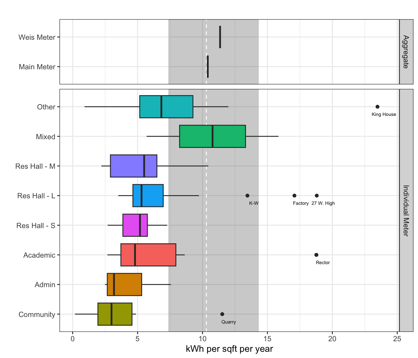
| Version | Author | Date |
|---|---|---|
| 92fcd5c | maggiedouglas | 2026-03-04 |
sessionInfo()R version 4.3.2 (2023-10-31)
Platform: x86_64-apple-darwin20 (64-bit)
Running under: macOS Ventura 13.7.8
Matrix products: default
BLAS: /Library/Frameworks/R.framework/Versions/4.3-x86_64/Resources/lib/libRblas.0.dylib
LAPACK: /Library/Frameworks/R.framework/Versions/4.3-x86_64/Resources/lib/libRlapack.dylib; LAPACK version 3.11.0
locale:
[1] en_US.UTF-8/en_US.UTF-8/en_US.UTF-8/C/en_US.UTF-8/en_US.UTF-8
time zone: America/New_York
tzcode source: internal
attached base packages:
[1] stats graphics grDevices utils datasets methods base
other attached packages:
[1] RColorBrewer_1.1-3 scales_1.3.0 DT_0.33 lubridate_1.9.3
[5] forcats_1.0.0 stringr_1.5.1 dplyr_1.1.4 purrr_1.0.2
[9] readr_2.1.5 tidyr_1.3.1 tibble_3.2.1 ggplot2_3.5.1
[13] tidyverse_2.0.0
loaded via a namespace (and not attached):
[1] sass_0.4.8 utf8_1.2.4 generics_0.1.3 stringi_1.8.3
[5] hms_1.1.3 digest_0.6.37 magrittr_2.0.3 timechange_0.3.0
[9] evaluate_0.23 grid_4.3.2 fastmap_1.1.1 rprojroot_2.0.4
[13] workflowr_1.7.1 jsonlite_1.8.8 whisker_0.4.1 promises_1.2.1
[17] fansi_1.0.6 crosstalk_1.2.1 jquerylib_0.1.4 cli_3.6.2
[21] rlang_1.1.3 ellipsis_0.3.2 munsell_0.5.0 withr_3.0.0
[25] cachem_1.0.8 yaml_2.3.8 tools_4.3.2 tzdb_0.4.0
[29] colorspace_2.1-0 httpuv_1.6.13 vctrs_0.6.5 R6_2.5.1
[33] lifecycle_1.0.4 git2r_0.33.0 htmlwidgets_1.6.4 fs_1.6.3
[37] pkgconfig_2.0.3 pillar_1.9.0 bslib_0.6.1 later_1.3.2
[41] gtable_0.3.4 glue_1.7.0 Rcpp_1.1.0 highr_0.10
[45] xfun_0.41 tidyselect_1.2.0 rstudioapi_0.16.0 knitr_1.45
[49] farver_2.1.1 htmltools_0.5.7 labeling_0.4.3 rmarkdown_2.25
[53] compiler_4.3.2