Campus building summary
Maggie Douglas
03/20/26
Load data
library(tidyverse)
library(DT) # library to create tables
library(scales) # library to format dollars
library(RColorBrewer)
library(paletteer)

is_outlier <- function(x) {
  return(x < quantile(x, 0.25, na.rm = T) - 1.5 * IQR(x, na.rm = T) | x > quantile(x, 0.75, na.rm = T) + 1.5 * IQR(x, na.rm = T))
}
daily_full <- read.csv("./output/kwh_daily_2026-03-17.csv") %>%
mutate(date = as_date(date)) # convert back to date
joined_full <- read.csv("./output/kwh_annual_2026-03-17.csv")
joined_acad <- read.csv("./output/kwh_academic_2026-03-17.csv")
total <- joined_full %>%
filter(meter != "Submeter" & type != "Res Hall - U" & type != "Solar") %>%
summarize(kwh = sum(kwh, na.rm = T),
kwh_corr = sum(kwh_corr, na.rm = T),
sqft = sum(sqft, na.rm = T)) %>%
mutate(kwh_sqft = kwh_corr/sqft,
meter = "Total")
total_acad <- joined_acad %>%
filter(meter != "Submeter" & type != "Res Hall - U" & type != "Solar") %>%
summarize(kwh = sum(kwh, na.rm = T),
kwh_corr = sum(kwh_corr, na.rm = T),
sqft = sum(sqft, na.rm = T)) %>%
mutate(kwh_sqft = kwh_corr/sqft,
meter = "Total")
buildings <- read.csv("./keys/fy25_building_list_updated.csv", strip.white = T) %>%
mutate(meter = ifelse(weis_meter == 1, "Weis Meter",
ifelse(main_meter == 0 & weis_meter == 0, "Individually Metered", "Main Meter")),
NAME = str_remove_all(NAME, "/"),
NAME = str_replace_all(NAME, " "," "),
NAME = str_replace_all(NAME, " "," "))
# store conversion factors
dollars_kwh <- 0.08138507
co2_kg_kwh <- 0.30082405# summarize # buildings by meter status
bldg_sum <- buildings %>%
filter(NAME != "Main Meter") %>%
group_by(meter) %>%
summarize(number = n())
bldg_tot <- bldg_sum %>%
summarize(number = sum(number)) %>%
mutate(meter = "Total")
bldg_comb <- rbind(bldg_sum, bldg_tot)
# summarize slightly differently for graphing
buildings_graph <- read.csv("./keys/fy25_building_list_updated.csv", strip.white = T) %>%
mutate(meter = ifelse(weis_meter == 1, "Weis Meter",
ifelse(main_meter == 1 & main_disagg == 0, "Main Meter",
ifelse(main_disagg == 1, "Submeter", "Individual")))) %>%
filter(!is.na(meter) & !type_new %in% c("Residential - U","Non-building","Solar"))
buildings_graph$meter <- factor(buildings_graph$meter,
levels = c("Weis Meter", "Main Meter",
"Submeter", "Individual"))
# generate summary for Main, Weis, and Individual meters
joined_agg <- joined_full %>%
ungroup() %>%
filter(meter != "Submeter" & type != "Res Hall - U" & type != "Solar") %>%
group_by(meter) %>%
summarize(kwh = sum(kwh, na.rm = T),
kwh_corr = sum(kwh_corr, na.rm = T),
sqft = sum(sqft, na.rm = T)) %>%
mutate(kwh_sqft = kwh_corr/sqft) %>%
rbind(total) %>%
mutate(dollars = kwh_corr*dollars_kwh,
ghg_MTCO2 = (kwh_corr*co2_kg_kwh)/1000) %>%
select(-kwh) %>%
arrange(kwh_corr)
joined_agg$meter <- factor(joined_agg$meter,
levels = c("Main Meter - Total",
"Weis Meter - Total",
"Individual", "Total"),
labels = c("Main Meter", "Weis Meter",
"Individually Metered","Total"))
joined_tot <- joined_agg %>%
left_join(bldg_comb, by = "meter")# generate summary by building category for individually metered buildings
joined_cat <- joined_full %>%
filter(meter %in% c("Individual","Submeter")) %>%
mutate(kwh_sqft = kwh_corr/sqft, # calculate kwh per sqft
kwh_person = kwh_corr/occupants,
dollars = kwh_corr*dollars_kwh,
ghg_kgCO2 = kwh_corr*co2_kg_kwh) %>%
group_by(type) %>%
summarize(n = n(),
kwh = sum(kwh_corr),
dollars = sum(dollars),
ghg_kgCO2 = sum(ghg_kgCO2),
sqft = median(sqft, na.rm = T),
med_kwh_sqft = median(kwh_sqft, na.rm = T),
kwh_sqft_25 = quantile(kwh_sqft, .25, na.rm = T),
kwh_sqft_75 = quantile(kwh_sqft, .75, na.rm = T)) %>%
arrange(-kwh)Background
This analysis examines electricity use on Dickinson’s campus as a whole in fiscal year 2025, to provide context for the category-specific analyses that follow. Buildings on Dickinson’s campus vary in how they are metered for electricity usage. Some buildings (and even individual apartments within buildings) have their own electricity meters, while others share a combined meter. There are two combined (or aggregate) meters - the “main meter” (associated with buildings in the central part of campus) and “Weis meter” (associated with buildings in a block around Weis Arts Complex). Some buildings on the main meter additionally have a “submeter” to track their individual electricity usage.
The electricity data analyzed here were derived from a combination of daily electricity use reported by the college electricity provider (PP&L) and daily electricity use recorded on submeters, both provided by the Center for Sustainability Education. Electricity data were fairly complete for the two aggregate meters and for buildings with individual meters (90-100% of days with data). Data for submetered buildings was more variable, with some buildings having >90% of days with usable data and other buildings having little to no usable data (see specific building categories for details).
Electricity use information was joined with information on building characteristics shared by Facilities. Electricity data for individual buildings is most available for residential buildings and ‘Other’ buildings (Figure 1 and 2), a category including assorted athletics buildings, faculty/staff residences, and auxillary buildings. Aggregate meters are prevalent for Academic, Administrative, and Community buildings (Figure 1 and 2). Once the data were joined, we summarized electricity use by building and calculated electricity use indicators including estimated financial cost, associated greenhouse gas emissions in metric tons of CO2-equivalents, and electricity use normalized by square footage and student occupancy (for residence halls only). Financial cost is a rough estimate based on per kWh supply and delivery charges in June 2025 for the main meter, a value that will underestimate cost for smaller buildings due to variable electricity costs. Greenhouse gas emissions are estimated using standard conversion factors based on a regional fuel blend for electricity (Leary 2025).
pal <- c("lightgrey","darkgrey","#CAB2D6","#6A3D9A")

ggplot(buildings_graph,
       aes(x = reorder(type_new, sqft, FUN = "sum"), fill = meter)) +
  geom_bar(position = "stack") +
  scale_fill_manual(values = pal) +
  theme_bw() +
  labs(x = "", y = "Number of buildings", fill = "Meter status",
       title = "Figure 1. Buildings by type and meter status") +
    theme(axis.text.x = element_text(angle = 45, vjust = 1, hjust = 1))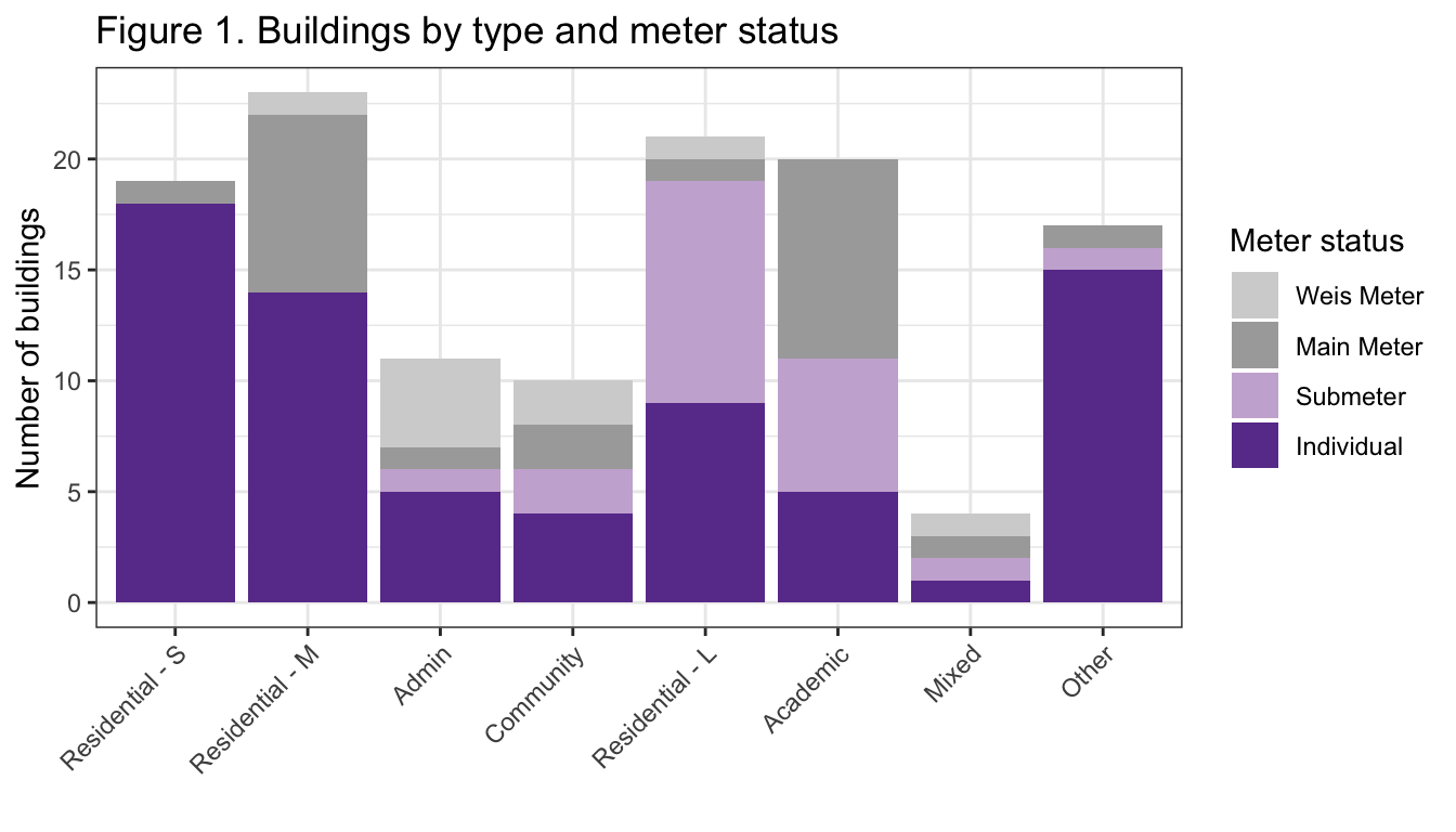
ggplot(buildings_graph,
       aes(x = reorder(type_new, sqft, FUN = "sum"), y = sqft/1000, fill = meter)) +
  geom_col(position = "stack") +
  scale_fill_manual(values = pal) +
  theme_bw() +
  labs(x = "", y = "Square Footage (1000)", fill = "Meter status",
       title = "Figure 2. Building square footage by type and meter status") +
    theme(axis.text.x = element_text(angle = 45, vjust = 1, hjust = 1))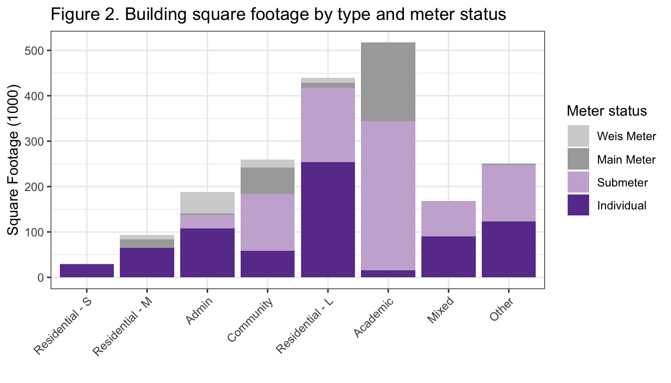
Electricity use summary
The analysis includes 134 distinct buildings, accounting for almost 2 million square feet of building space (Table 1, Figure 1). The majority (59%) of square footage was accounted for by buildings connected to the main meter (Table 1). We identified 44 distinct buildings on the main meter, a value that differs slightly from internal campus estimate of 37 buildings due to differences in how buildings are delineated in the two datasets (e.g. Rector Science Center and Tome are listed together in the electricity data but separately in the building data). Our final dataset also includes 81 individually metered buildings that together account for 36% of campus square footage.
We estimate that Dickinson used roughly 17 million kWh of electricity in fiscal year 2025, corresponding to a cost of roughly $1.4 million and over 5000 MT CO2-equivalents (Table 1). Most (68%) of this use was associated with buildings on the main meter. Another 6% was associated for nine buildings on the Weis meter, and the remaining 26% was associated with individually metered buildings.
joined_pretty_tot <- joined_tot %>%
  mutate(kwh = round(kwh_corr, digits = 0),
         dollars = paste("$",round(dollars, digits = 0)),
         ghg_MTCO2 = round(ghg_MTCO2, digits = 0),
         sqft = round(sqft, digits = 0),
         kwh_sqft = round(kwh_sqft, digits = 1)) %>%
  select(meter, number, sqft, kwh, dollars, ghg_MTCO2, kwh_sqft) %>%
  arrange(kwh)

joined_pretty_cat <- joined_cat %>%
  mutate(kwh = round(kwh, digits = 0),
         dollars = paste("$",round(dollars, digits = 0)),
         ghg_MTCO2 = round(ghg_kgCO2/1000, digits = 0),
         sqft = round(sqft, digits = 0),
         med_kwh_sqft = round(med_kwh_sqft, digits = 1),
         kwh_sqft_25 = round(kwh_sqft_25, digits = 1),
         kwh_sqft_75 = round(kwh_sqft_75, digits = 1)) %>%
    select(type, n, sqft, med_kwh_sqft, kwh_sqft_25, kwh_sqft_75) %>%
  arrange(desc(med_kwh_sqft)) %>%
  filter(!is.na(med_kwh_sqft))
datatable(joined_pretty_tot,
rownames = FALSE,
colnames = c("Meter status","Buildings", "Square\nfootage", "kWh", "Est. cost",
"CO2e\n(MT)", "kWh per\nsqft"),
filter = "none",
class = "compact",
options = list(pageLength = 4, autoWidth = TRUE, dom = 't'),
caption = "Table 1. Building and electricity summary by meter status in Fiscal Year 2025. Annual estimates for each meter were adjusted to account for missing days of electricity data.")datatable(joined_pretty_cat,
rownames = FALSE,
colnames = c("Building\ntype","Buildings\nwith data", "Median\nsquare\nfootage", "Median\nkWh\nper sqft",
"25th Perc.", "75th Perc."),
filter = "none",
class = "compact",
options = list(pageLength = 11, autoWidth = TRUE, dom = 't'),
caption = "Table 2. Descriptive statistics for annual electricity use by building type for those buildings with individual electricity use data (n = 81 buildings). Annual estimates for each meter were adjusted to account for missing days of electricity data.")Electricity use over the year
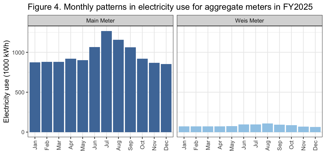
Electricity use peaked in July and was lowest in May and November (Figure 3). At all times of year, buildings on the main meter accounted for most of the electricity use, and the main meter buildings appeared to drive the seasonal pattern (Figure 4). Of the individually metered buildings, large residence halls accounted for the largest share of electricity use and peaked in winter (Figure 5). Interestingly, electricity production through the solar field peaked in July and was lowest in December and January (Figure 3).
daily_graph <- daily_full %>%
  mutate(date = as_date(date),
         month = month(date, label = TRUE),
         day = wday(date, label = TRUE),
         type_brief = recode(type,
                       'Res Hall - U' = 'Residential',
                       'Res Hall - S' = 'Residential',
                       'Res Hall - M' = 'Residential',
                       'Res Hall - L' = 'Residential')) %>%
  filter(!is.na(month))

ggplot(filter(daily_graph, meter != "Submeter"),
       aes(x = month, y = kwh/10^6, fill = reorder(type_brief, kwh, FUN = sum))) +
  geom_col(position = "stack") +
  scale_fill_paletteer_d("ggthemes::Tableau_20") +
  #scale_fill_brewer(type = "qual", palette = "Paired") +
  theme_bw() +
  labs(x = "", y = "Electricity use (million kWh)", fill = "",
       title = "Figure 3. Monthly patterns in electricity use in FY25")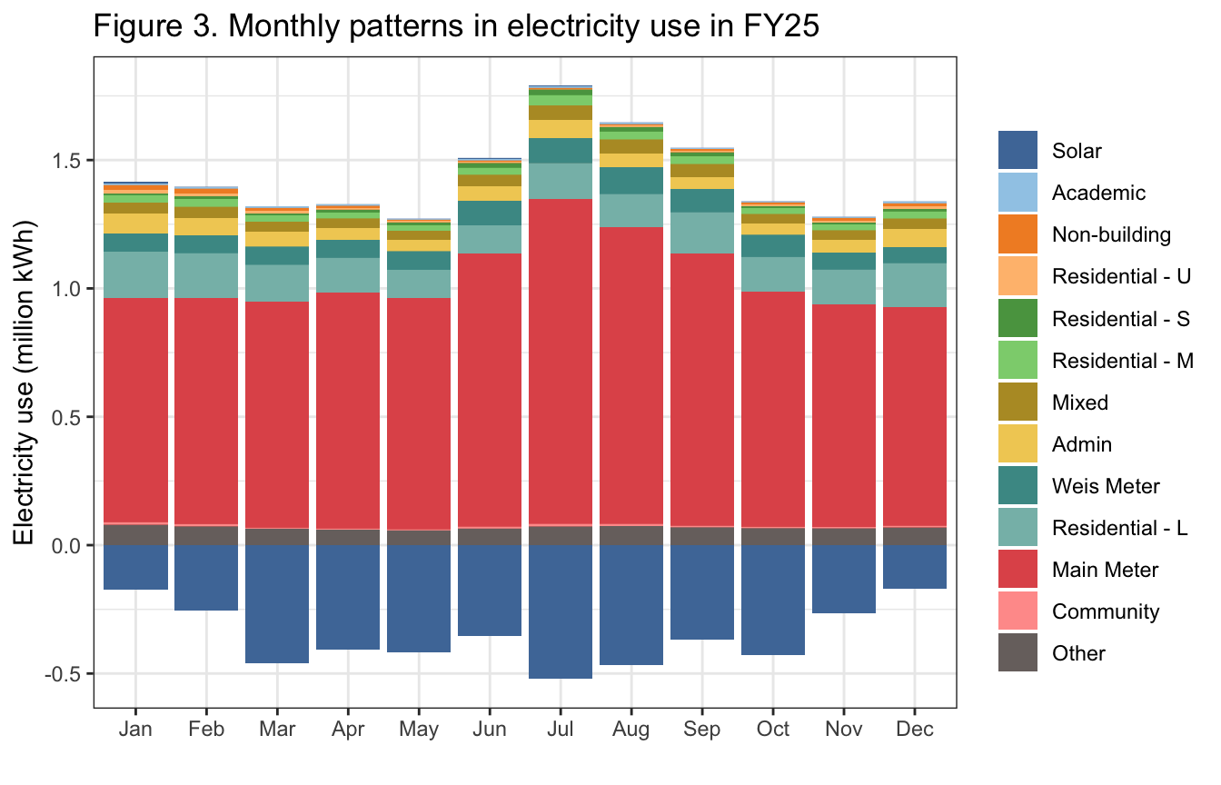
ggplot(filter(daily_graph, meter %in% c("Main Meter - Total", "Weis Meter - Total")),
       aes(x = month, y = kwh/10^3, fill = type_brief)) +
  geom_col(position = "stack") +
  facet_wrap(. ~ type_brief) +
  scale_fill_paletteer_d("ggthemes::Tableau_20") +
  theme_bw() +
  theme(legend.position = "none") +
  theme(axis.text.x = element_text(angle = 90, vjust = 0.5, hjust = 1)) +
  labs(x = "", y = "Electricity use (1000 kWh)", fill = "",
       title = "Figure 4. Monthly patterns in electricity use for aggregate meters in FY2025",
       )
ggplot(filter(daily_graph, meter == "Individual" & type != "Solar"),
       aes(x = month, y = kwh/10^3, fill = type_brief)) +
  geom_col(position = "stack") +
  facet_wrap(. ~ type_brief) +
  scale_fill_paletteer_d("ggthemes::Tableau_20") +
  theme_bw() +
  theme(legend.position = "none") +
  theme(axis.text.x = element_text(angle = 90, vjust = 0.5, hjust = 1)) +
  labs(x = "", y = "Electricity use (1000 kWh)", fill = "",
       title = "Figure 5. Monthly patterns in electricity use by category in FY2025",
       subtitle = "Only includes buildings with individual meters. Most electricity use is on the Main Meter.")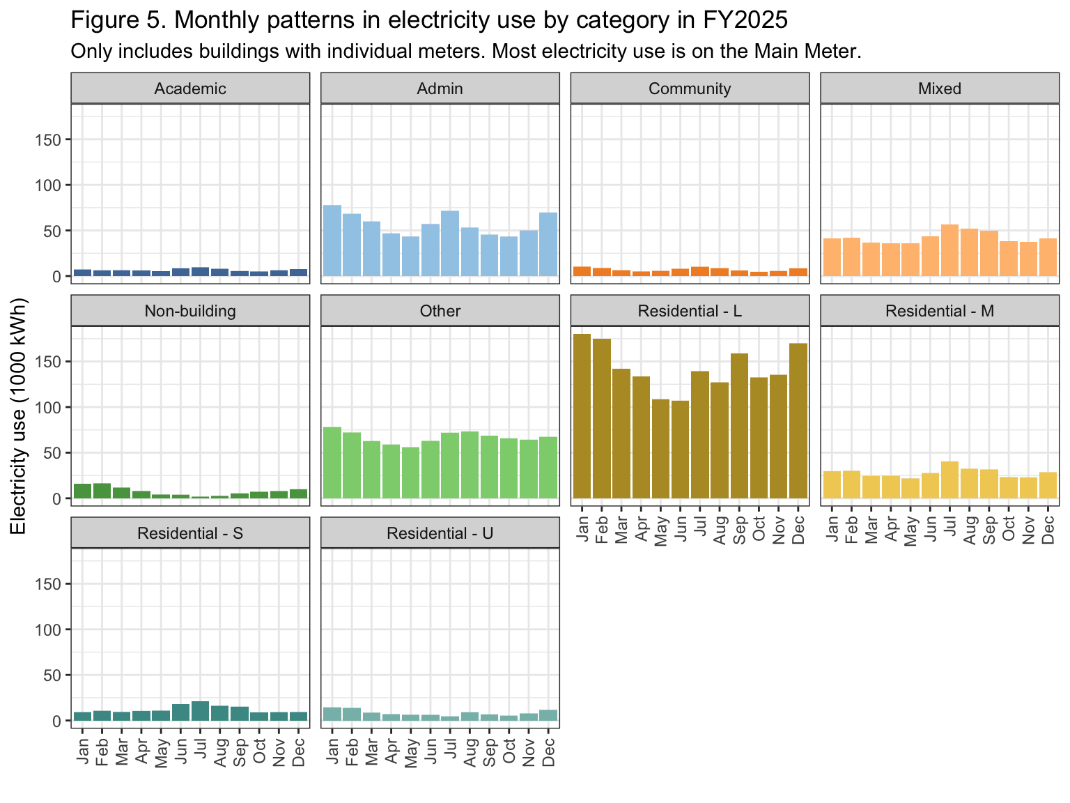
Electricity intensity
Looking at the entire fiscal year, electricity intensity (use per square foot of space) varied across building categories for individually metered buildings (Table 2, Figure 5). Administrative buildings had the lowest electricity intensity with a median of 3.2 kWh/sqft (interquartile range 2.6-5.3 kWh/sqft), while the ‘Mixed’ category of buildings had the highest value at 15.6 kWh/sqft (interquartile range 10.7-20.6 kWh/sqft). Importantly, the ‘Mixed’ category includes Kaufman Hall, which houses the campus central energy plant and supplies heat and cooling to other buildings on campus. That said, electricity intensity for most individually metered buildings was substantially below typical values for U.S. Colleges and Universities as reported by the U.S. Energy Information Administration (EIA 2022).
Interestingly, the two aggregate meters that account for most electricity use on campus had a slightly higher electricity intensity than most individually metered buildings, at 11.4 kWh/sqft for buildings on the Weis meter and 10.4 kWh/sqft for buildings on the main meter (Table 1, Figure 5). These values are very close to the median value of 10.3 kWh/sqft (interquartile range 7.4-14.3 kWh/sqft) reported for U.S. Colleges and Universities (EIA 2022).
Values for the academic year only showed a more pronounced trend of falling below the values for typical U.S. College and University buildings, for both the aggregate meters and the buildings on individual meters (Figure 7).
It is also worth noting that values for the
intensity <- joined_full %>%
  filter(!(type %in% c("Residential - U","Solar", "Non-building"))) %>%
  mutate(kwh_sqft = kwh_corr/sqft,
         meter_type = ifelse(type %in% c("Main Meter","Weis Meter"), "Aggregate", "Individual Meter"),
         outlier = case_when(
           NAME == "King House" ~ "King House",
           NAME == "Kisner - Woodward" ~ "K-W",
           NAME == "Factory Apts." ~ "Factory",
           NAME == "Rector Science Center" ~ "Rector",
           NAME == "Quarry, The " ~ "Quarry",
           NAME == "27 W. High St." ~ "27 W. High"
         ))

# median and IQR come from EIA (2022) table, annual kWh per square foot for Colleges/Universities
# https://www.eia.gov/consumption/commercial/data/2018/ce/pdf/c22.pdf

ggplot(intensity,
       aes(x = reorder(type, kwh_sqft, FUN = "median"),
                        y = kwh_sqft, fill = type)) +
  annotate("rect", xmin = -Inf, xmax = Inf, ymin = 7.4, ymax = 14.3, color = "lightgray", alpha = 0.3) +
  geom_hline(yintercept = 10.3, linetype = "dashed", color = "white") +
  facet_grid(meter_type ~ ., scales = "free_y", space = "free_y") +
  geom_boxplot() +
  geom_label(aes(label = outlier), na.rm = TRUE, nudge_x = -0.25, nudge_y = 0.5,
             color = "black", fill = "white", size = 2, alpha = 0, label.size = NA) +
    scale_fill_paletteer_d("ggthemes::Tableau_20") +
  ylim(0, 25) +
  coord_flip() +
  theme_bw() +
  theme(legend.position = "none") +
  labs(x = "", y = "Electricity Intensity (kWh/sqft/year)",
       title = "Figure 6. Electricity intensity by meter/building category in FY25",
       caption = "White dotted line and gray shaded area show median and 25th to 75th percentile \nof typical values in U.S. College and University buildings (EIA 2022)")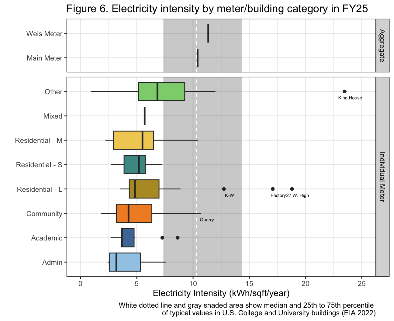
intensity_acad <- joined_acad %>%
  filter(!(type %in% c("Residential - U","Solar", "Non-building"))) %>%
    mutate(kwh_sqft = kwh_corr/sqft,
         meter_type = ifelse(type %in% c("Main Meter","Weis Meter"), "Aggregate", "Individual Meter"))

ggplot(intensity_acad,
       aes(x = reorder(type, kwh_sqft, FUN = "median"),
                        y = kwh_sqft, fill = type)) +
  annotate("rect", xmin = -Inf, xmax = Inf, ymin = 7.4, ymax = 14.3, color = "lightgray", alpha = 0.3) +
  geom_hline(yintercept = 10.3, linetype = "dashed", color = "white") +
  facet_grid(meter_type ~ ., scales = "free_y", space = "free_y") +
    scale_fill_paletteer_d("ggthemes::Tableau_20") +
    ylim(0, 25) +
  geom_boxplot() +
  coord_flip() +
  theme_bw() +
  theme(legend.position = "none") +
  labs(x = "", y = "Electricity Intensity (kWh/sqft/year)",
       title = "Figure 7. Electricity intensity by meter/building category in AY24/25",
       caption = "White dotted line and gray shaded area show median and 25th to 75th percentile \nof typical values in U.S. College and University buildings (EIA 2022)")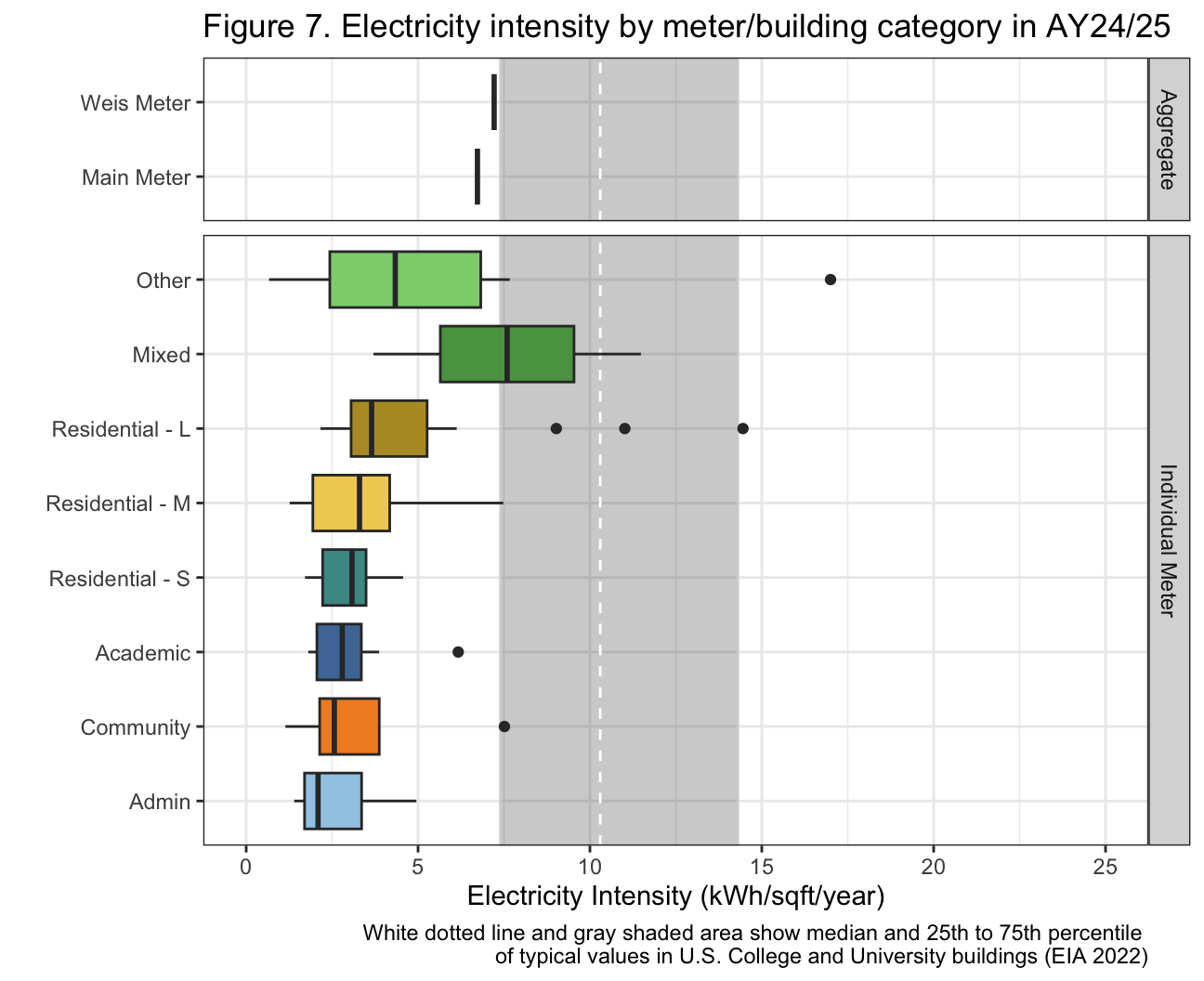
Recommendations
TBD!
Sources
Energy Information Administration (EIA). (2022). 2018 Commercial Buildings Energy Consumption Survey (CBECS). https://www.eia.gov/consumption/commercial/
Leary, N. (2025). Dickinson College Greenhouse Gas Inventory 2008-2023. Center for Sustainability Education.
sessionInfo()R version 4.5.2 (2025-10-31)
Platform: x86_64-apple-darwin20
Running under: macOS Ventura 13.7.8
Matrix products: default
BLAS: /Library/Frameworks/R.framework/Versions/4.5-x86_64/Resources/lib/libRblas.0.dylib
LAPACK: /Library/Frameworks/R.framework/Versions/4.5-x86_64/Resources/lib/libRlapack.dylib; LAPACK version 3.12.1
locale:
[1] en_US.UTF-8/en_US.UTF-8/en_US.UTF-8/C/en_US.UTF-8/en_US.UTF-8
time zone: America/New_York
tzcode source: internal
attached base packages:
[1] stats graphics grDevices utils datasets methods base
other attached packages:
[1] paletteer_1.7.0 RColorBrewer_1.1-3 scales_1.4.0 DT_0.34.0
[5] lubridate_1.9.5 forcats_1.0.1 stringr_1.6.0 dplyr_1.2.0
[9] purrr_1.2.1 readr_2.2.0 tidyr_1.3.2 tibble_3.3.1
[13] ggplot2_4.0.2 tidyverse_2.0.0
loaded via a namespace (and not attached):
[1] sass_0.4.10 generics_0.1.4 prismatic_1.1.2 stringi_1.8.7
[5] hms_1.1.4 digest_0.6.39 magrittr_2.0.4 timechange_0.4.0
[9] evaluate_1.0.5 grid_4.5.2 fastmap_1.2.0 rprojroot_2.1.1
[13] workflowr_1.7.2 jsonlite_2.0.0 whisker_0.4.1 rematch2_2.1.2
[17] promises_1.5.0 crosstalk_1.2.2 jquerylib_0.1.4 cli_3.6.5
[21] rlang_1.1.7 withr_3.0.2 cachem_1.1.0 yaml_2.3.12
[25] otel_0.2.0 tools_4.5.2 tzdb_0.5.0 httpuv_1.6.16
[29] vctrs_0.7.1 R6_2.6.1 lifecycle_1.0.5 git2r_0.36.2
[33] htmlwidgets_1.6.4 fs_1.6.7 pkgconfig_2.0.3 pillar_1.11.1
[37] bslib_0.10.0 later_1.4.8 gtable_0.3.6 glue_1.8.0
[41] Rcpp_1.1.1 xfun_0.56 tidyselect_1.2.1 rstudioapi_0.18.0
[45] knitr_1.51 farver_2.1.2 htmltools_0.5.9 labeling_0.4.3
[49] rmarkdown_2.30 compiler_4.5.2 S7_0.2.1