Campus building summary
Maggie Douglas
2026-03-04
Last updated: 2026-03-04
Checks: 6 1
Knit directory: dickinson_power/
This reproducible R Markdown analysis was created with workflowr (version 1.7.1). The Checks tab describes the reproducibility checks that were applied when the results were created. The Past versions tab lists the development history.
The R Markdown file has unstaged changes. To know which version of
the R Markdown file created these results, you’ll want to first commit
it to the Git repo. If you’re still working on the analysis, you can
ignore this warning. When you’re finished, you can run
wflow_publish to commit the R Markdown file and build the
HTML.
Great job! The global environment was empty. Objects defined in the global environment can affect the analysis in your R Markdown file in unknown ways. For reproduciblity it’s best to always run the code in an empty environment.
The command set.seed(20260107) was run prior to running
the code in the R Markdown file. Setting a seed ensures that any results
that rely on randomness, e.g. subsampling or permutations, are
reproducible.
Great job! Recording the operating system, R version, and package versions is critical for reproducibility.
Nice! There were no cached chunks for this analysis, so you can be confident that you successfully produced the results during this run.
Great job! Using relative paths to the files within your workflowr project makes it easier to run your code on other machines.
Great! You are using Git for version control. Tracking code development and connecting the code version to the results is critical for reproducibility.
The results in this page were generated with repository version 0332ba1. See the Past versions tab to see a history of the changes made to the R Markdown and HTML files.
Note that you need to be careful to ensure that all relevant files for
the analysis have been committed to Git prior to generating the results
(you can use wflow_publish or
wflow_git_commit). workflowr only checks the R Markdown
file, but you know if there are other scripts or data files that it
depends on. Below is the status of the Git repository when the results
were generated:
Ignored files:
    Ignored:    .DS_Store
    Ignored:    .Rhistory
    Ignored:    .Rproj.user/
    Ignored:    data/.DS_Store
    Ignored:    data/FY25 Main Meter Data.xlsx
    Ignored:    data/building_list_FY25_updated.xlsx
    Ignored:    data/graph_data_life_exp.csv
    Ignored:    data/housing_counts.csv
    Ignored:    keys/.DS_Store
    Ignored:    output/building_check.csv
    Ignored:    output/building_check.xlsx
    Ignored:    output/kwh_annual.csv
    Ignored:    output/kwh_annual_2026-03-04.csv
    Ignored:    output/kwh_annual_20260225.csv
    Ignored:    output/kwh_annual_20260226.csv
    Ignored:    output/kwh_daily.csv
    Ignored:    output/kwh_daily_2026-03-04.csv
    Ignored:    output/kwh_daily_20260225.csv
    Ignored:    output/kwh_daily_20260226.csv
    Ignored:    output/kwh_main_annual.csv
    Ignored:    output/kwh_main_daily.csv

Unstaged changes:
    Modified:   analysis/_site.yml
    Modified:   analysis/campus_summary.Rmd
Note that any generated files, e.g. HTML, png, CSS, etc., are not included in this status report because it is ok for generated content to have uncommitted changes.
These are the previous versions of the repository in which changes were
made to the R Markdown (analysis/campus_summary.Rmd) and
HTML (docs/campus_summary.html) files. If you’ve configured
a remote Git repository (see ?wflow_git_remote), click on
the hyperlinks in the table below to view the files as they were in that
past version.
| File | Version | Author | Date | Message |
|---|---|---|---|---|
| Rmd | bfe7b73 | maggiedouglas | 2026-03-04 | fix data wrangling! |
| Rmd | d04b276 | maggiedouglas | 2026-03-04 | fix data wrangling! |
Load data
library(tidyverse)── Attaching core tidyverse packages ──────────────────────── tidyverse 2.0.0 ──
✔ dplyr 1.1.4 ✔ readr 2.1.5
✔ forcats 1.0.0 ✔ stringr 1.5.1
✔ ggplot2 3.5.1 ✔ tibble 3.2.1
✔ lubridate 1.9.3 ✔ tidyr 1.3.1
✔ purrr 1.0.2
── Conflicts ────────────────────────────────────────── tidyverse_conflicts() ──
✖ dplyr::filter() masks stats::filter()
✖ dplyr::lag() masks stats::lag()
ℹ Use the conflicted package (<http://conflicted.r-lib.org/>) to force all conflicts to become errorslibrary(DT) # library to create tables
library(scales) # library to format dollars
Attaching package: 'scales'

The following object is masked from 'package:purrr':

    discard

The following object is masked from 'package:readr':

col_factorlibrary(RColorBrewer)daily_full <- read.csv("./output/kwh_daily_2026-03-04.csv") %>%
mutate(date = as_date(date)) # convert back to date
joined_full <- read.csv("./output/kwh_annual_2026-03-04.csv")
# store conversion factors
dollars_kwh <- 0.08138507
co2_kg_kwh <- 0.30082405# generate summary by building category
joined_cat <- joined_full %>%
mutate(kwh_sqft = kwh_corr/sqft, # calculate kwh per sqft
kwh_person = kwh_corr/occupants,
dollars = kwh_corr*dollars_kwh,
ghg_kgCO2 = kwh_corr*co2_kg_kwh) %>%
group_by(type) %>%
summarize(n = n(),
kwh = sum(kwh_corr),
dollars = sum(dollars),
ghg_kgCO2 = sum(ghg_kgCO2),
sqft = sum(sqft, na.rm = T),
med_kwh_sqft = median(kwh_sqft, na.rm = T),
kwh_sqft_25 = quantile(kwh_sqft, .25, na.rm = T),
kwh_sqft_75 = quantile(kwh_sqft, .75, na.rm = T)) %>%
arrange(-kwh)Building type summary
Electricity use summary
joined_pretty_cat <- joined_cat %>%
  mutate(n = ifelse(n == 1, "-", n),
         kwh = round(kwh, digits = 0),
         dollars = paste("$",round(dollars, digits = 0)),
         ghg_MTCO2 = round(ghg_kgCO2/1000, digits = 0),
         sqft = round(sqft, digits = 0),
         med_kwh_sqft = round(med_kwh_sqft, digits = 1),
         kwh_sqft_25 = round(kwh_sqft_25, digits = 1),
         kwh_sqft_75 = round(kwh_sqft_75, digits = 1)) %>%
    select(type, n, kwh, dollars, ghg_MTCO2, sqft, med_kwh_sqft, kwh_sqft_25, kwh_sqft_75) %>%
  arrange(desc(med_kwh_sqft))
datatable(joined_pretty_cat,
filter = 'top',
rownames = FALSE,
colnames = c("Building\ntype","Buildings\nwith data", "kWh", "Est. cost",
"CO2e\n(MT)", "Square\nfootage", "Median\nkWh\nper sqft",
"25th Perc.", "75th Perc."),
caption = "Table 1. Descriptive statistics for annual electricity use by building type. Annual estimates for each building/meter were generated by multiplying daily mean values by 365 days in the year. Those estimates were then summarized here.")Electricity use over the year
daily_graph <- daily_full %>%
  mutate(date = as_date(date),
         month = month(date, label = TRUE),
         day = wday(date, label = TRUE),
         type_brief = recode(type,
                       'Res Hall - U' = 'Res Hall',
                       'Res Hall - S' = 'Res Hall',
                       'Res Hall - M' = 'Res Hall',
                       'Res Hall - L' = 'Res Hall')) %>%
  filter(!is.na(month))

ggplot(filter(daily_graph, meter != "Submeter"),
       aes(x = month, y = kwh/10^6, fill = reorder(type_brief, kwh, FUN = sum))) +
  geom_col(position = "stack") +
  scale_fill_brewer(type = "qual", palette = "Paired") +
  theme_bw() +
  labs(x = "", y = "Electricity use (million kWh)", fill = "",
       title = "Electricity use by building type")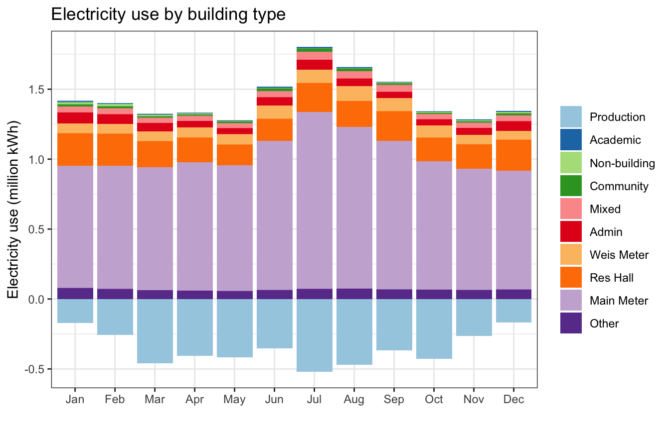
Submeter data
ggplot(filter(daily_graph, meter == "Submeter"),
       aes(x = month, y = kwh/10^6, fill = reorder(type_brief, kwh, FUN = sum))) +
  geom_col(position = "stack") +
  scale_fill_brewer(type = "qual", palette = "Paired") +
  theme_bw() +
  labs(x = "", y = "Electricity use (million kWh)", fill = "",
       title = "Electricity data from the submeters")
Warning: Removed 1876 rows containing missing values or values outside the scale range
(`geom_col()`).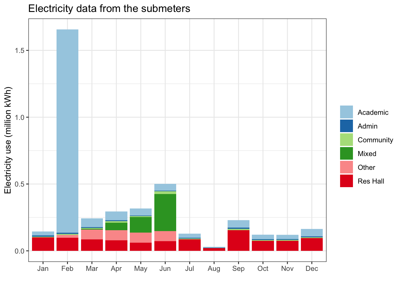
ggplot(daily_graph, aes(x = month, y = kwh/10^6, fill = reorder(type, kwh, FUN = 'sum'))) +
  geom_col(position = "stack") +
  facet_wrap(. ~ type, scales = "free") +
  theme_bw() +
  labs(x = "", y = "Electricity use (million kWh)", fill = "") +
  theme(axis.text.x = element_text(angle = 90, hjust = 1, vjust = 0.5)) +
  theme(legend.position = "none")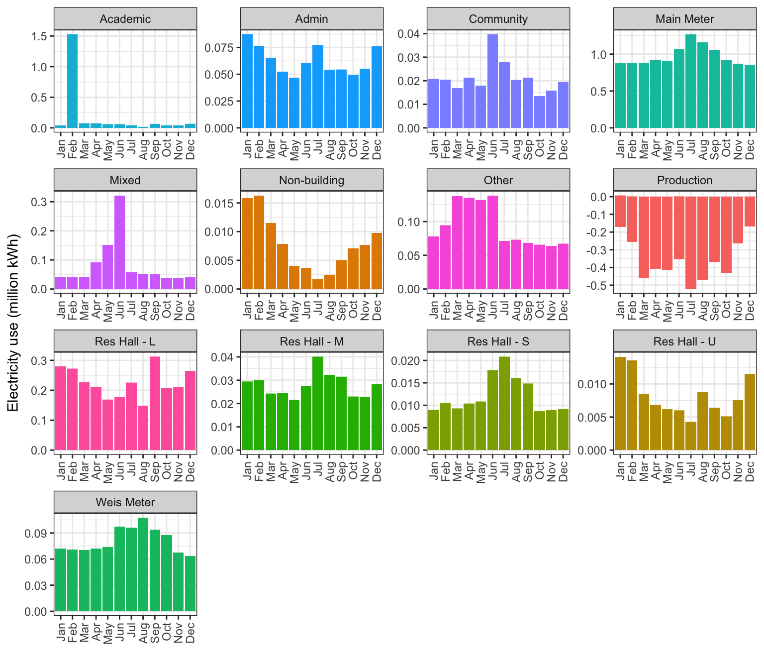
Electricity intensity by type
to_exclude <- filter(joined_full, days_perc < 90)

intensity <- joined_full %>%
  filter(!(type %in% c("Res Hall - U","Production", "Non-building"))) %>%
  mutate(kwh_sqft = kwh_corr/sqft,
         meter_type = ifelse(type %in% c("Main Meter","Weis Meter"), "Agg.", "Individual"))

# median and IQR come from EIA (2022) table, annual kWh per square foot for Colleges/Universities
# https://www.eia.gov/consumption/commercial/data/2018/ce/pdf/c22.pdf

ggplot(intensity,
       aes(x = reorder(type, kwh_sqft, FUN = "median"),
                        y = kwh_sqft, fill = type)) +
  annotate("rect", xmin = -Inf, xmax = Inf, ymin = 7.4, ymax = 14.3, color = "lightgray", alpha = 0.3) +
  geom_hline(yintercept = 10.3, linetype = "dashed", color = "white") +
  facet_grid(meter_type ~ ., scales = "free_y", space = "free_y") +
  geom_boxplot() +
  coord_flip() +
  theme_bw() +
  theme(legend.position = "none") +
  labs(x = "", y = "kWh per sqft per year",
       title = "Electricity Intensity by Building Type")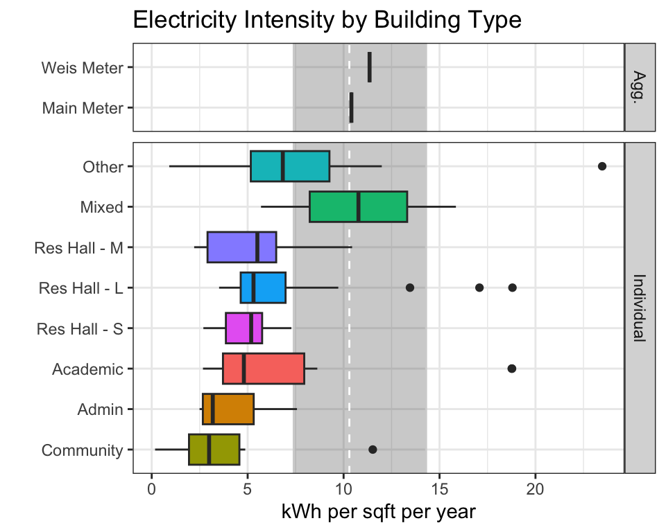
Summary statistics
summary(joined_full) type meter NAME days_perc
Length:104 Length:104 Length:104 Min. : 36.71
Class :character Class :character Class :character 1st Qu.: 95.34
Mode :character Mode :character Mode :character Median :100.00
Mean : 95.72
3rd Qu.:100.00
Max. :100.00
kwh kwh_corr sqft occupants
Min. :-4274284 Min. :-4274284 Min. : 500 Min. : 1.50
1st Qu.: 8249 1st Qu.: 8249 1st Qu.: 1925 1st Qu.: 5.00
Median : 20783 Median : 21273 Median : 5912 Median : 9.50
Mean : 162525 Mean : 203347 Mean : 30890 Mean : 33.14
3rd Qu.: 88355 3rd Qu.: 88355 3rd Qu.: 24421 3rd Qu.: 40.88
Max. :11648808 Max. :11648808 Max. :1119435 Max. :161.50
NA's :14 NA's :46 ## Stats for campus buildings
stats <- filter(joined_full, meter != "Submeter" & type != "Production")
# million square feet
sum(stats$kwh)/10^6 # million kwh[1] 17.23632sum(stats$dollars)/10^6 # million $[1] 0sum(stats$ghg_kgCO2)/1000 # MT CO2e[1] 0## Stats for solar
solar <- filter(joined_full, type == "Production")
sum(solar$kwh)/10^6 # million kwh[1] -4.274285sum(solar$dollars)/10^6 # million $[1] 0sum(solar$ghg_kgCO2)/1000 # MT CO2e[1] 0
sessionInfo()R version 4.3.2 (2023-10-31)
Platform: x86_64-apple-darwin20 (64-bit)
Running under: macOS Ventura 13.7.8
Matrix products: default
BLAS: /Library/Frameworks/R.framework/Versions/4.3-x86_64/Resources/lib/libRblas.0.dylib
LAPACK: /Library/Frameworks/R.framework/Versions/4.3-x86_64/Resources/lib/libRlapack.dylib; LAPACK version 3.11.0
locale:
[1] en_US.UTF-8/en_US.UTF-8/en_US.UTF-8/C/en_US.UTF-8/en_US.UTF-8
time zone: America/New_York
tzcode source: internal
attached base packages:
[1] stats graphics grDevices utils datasets methods base
other attached packages:
[1] RColorBrewer_1.1-3 scales_1.3.0 DT_0.33 lubridate_1.9.3
[5] forcats_1.0.0 stringr_1.5.1 dplyr_1.1.4 purrr_1.0.2
[9] readr_2.1.5 tidyr_1.3.1 tibble_3.2.1 ggplot2_3.5.1
[13] tidyverse_2.0.0
loaded via a namespace (and not attached):
[1] sass_0.4.8 utf8_1.2.4 generics_0.1.3 stringi_1.8.3
[5] hms_1.1.3 digest_0.6.37 magrittr_2.0.3 timechange_0.3.0
[9] evaluate_0.23 grid_4.3.2 fastmap_1.1.1 rprojroot_2.0.4
[13] workflowr_1.7.1 jsonlite_1.8.8 whisker_0.4.1 promises_1.2.1
[17] fansi_1.0.6 crosstalk_1.2.1 jquerylib_0.1.4 cli_3.6.2
[21] rlang_1.1.3 ellipsis_0.3.2 munsell_0.5.0 withr_3.0.0
[25] cachem_1.0.8 yaml_2.3.8 tools_4.3.2 tzdb_0.4.0
[29] colorspace_2.1-0 httpuv_1.6.13 vctrs_0.6.5 R6_2.5.1
[33] lifecycle_1.0.4 git2r_0.33.0 htmlwidgets_1.6.4 fs_1.6.3
[37] pkgconfig_2.0.3 pillar_1.9.0 bslib_0.6.1 later_1.3.2
[41] gtable_0.3.4 glue_1.7.0 Rcpp_1.1.0 highr_0.10
[45] xfun_0.41 tidyselect_1.2.0 rstudioapi_0.16.0 knitr_1.45
[49] farver_2.1.1 htmltools_0.5.7 labeling_0.4.3 rmarkdown_2.25
[53] compiler_4.3.2