PS 5: Preliminary results
Claire Raesly and Liv Kacar
2026-03-04
Last updated: 2026-03-12
Checks: 6 1
Knit directory: dickinson_power/
This reproducible R Markdown analysis was created with workflowr (version 1.7.2). The Checks tab describes the reproducibility checks that were applied when the results were created. The Past versions tab lists the development history.
The R Markdown file has unstaged changes. To know which version of
the R Markdown file created these results, you’ll want to first commit
it to the Git repo. If you’re still working on the analysis, you can
ignore this warning. When you’re finished, you can run
wflow_publish to commit the R Markdown file and build the
HTML.
Great job! The global environment was empty. Objects defined in the global environment can affect the analysis in your R Markdown file in unknown ways. For reproduciblity it’s best to always run the code in an empty environment.
The command set.seed(20260107) was run prior to running
the code in the R Markdown file. Setting a seed ensures that any results
that rely on randomness, e.g. subsampling or permutations, are
reproducible.
Great job! Recording the operating system, R version, and package versions is critical for reproducibility.
Nice! There were no cached chunks for this analysis, so you can be confident that you successfully produced the results during this run.
Great job! Using relative paths to the files within your workflowr project makes it easier to run your code on other machines.
Great! You are using Git for version control. Tracking code development and connecting the code version to the results is critical for reproducibility.
The results in this page were generated with repository version 0a9f663. See the Past versions tab to see a history of the changes made to the R Markdown and HTML files.
Note that you need to be careful to ensure that all relevant files for
the analysis have been committed to Git prior to generating the results
(you can use wflow_publish or
wflow_git_commit). workflowr only checks the R Markdown
file, but you know if there are other scripts or data files that it
depends on. Below is the status of the Git repository when the results
were generated:
Ignored files:
    Ignored:    .DS_Store
    Ignored:    .Rhistory
    Ignored:    .Rproj.user/
    Ignored:    analysis/.DS_Store
    Ignored:    analysis_to-fix/.DS_Store
    Ignored:    data/.DS_Store
    Ignored:    data/FY25 Main Meter Data.xlsx
    Ignored:    data/building_list_FY25_updated.xlsx
    Ignored:    data/graph_data_life_exp.csv
    Ignored:    data/housing_counts.csv
    Ignored:    keys/.DS_Store
    Ignored:    output/annual_kwh.csv
    Ignored:    output/building_check.csv
    Ignored:    output/building_check.xlsx
    Ignored:    output/daily_kwh.csv
    Ignored:    output/kwh_annual.csv
    Ignored:    output/kwh_annual_2026-03-04.csv
    Ignored:    output/kwh_annual_20260225.csv
    Ignored:    output/kwh_annual_20260226.csv
    Ignored:    output/kwh_daily.csv
    Ignored:    output/kwh_daily_2026-03-04.csv
    Ignored:    output/kwh_daily_20260225.csv
    Ignored:    output/kwh_daily_20260226.csv
    Ignored:    output/kwh_main_annual.csv
    Ignored:    output/kwh_main_daily.csv

Untracked files:
    Untracked:  analysis/main_meter_case_study.Rmd
    Untracked:  analysis/main_meter_model.Rmd

Unstaged changes:
    Modified:   analysis/PS05_prelim_results_Res_Hall_L.Rmd
    Deleted:    analysis_to-fix/main_meter_case_study.Rmd
Note that any generated files, e.g. HTML, png, CSS, etc., are not included in this status report because it is ok for generated content to have uncommitted changes.
These are the previous versions of the repository in which changes were
made to the R Markdown
(analysis/PS05_prelim_results_Res_Hall_L.Rmd) and HTML
(docs/PS05_prelim_results_Res_Hall_L.html) files. If you’ve
configured a remote Git repository (see ?wflow_git_remote),
click on the hyperlinks in the table below to view the files as they
were in that past version.
| File | Version | Author | Date | Message |
|---|---|---|---|---|
| Rmd | 0a9f663 | maggiedouglas | 2026-03-11 | added alternate versions for stacked bar graphs - large Res Halls |
| html | 0a9f663 | maggiedouglas | 2026-03-11 | added alternate versions for stacked bar graphs - large Res Halls |
| Rmd | 38132bb | maggiedouglas | 2026-03-11 | add student draft results |
| html | 38132bb | maggiedouglas | 2026-03-11 | add student draft results |
Data preparation
Libraries
library(tidyverse)
library(DT)
library(paletteer)

is_outlier <- function(x) {
  return(x < quantile(x, 0.25, na.rm = T) - 1.5 * IQR(x, na.rm = T) | x > quantile(x, 0.75, na.rm = T) + 1.5 * IQR(x, na.rm = T))
}
Annual electricity data
annual <- read.csv("./output/kwh_annual_2026-03-04.csv")

str(annual)

cost_conversion <- 0.08138507
ghg_conversion <- 0.30082405 / 1000

annual_large_res <- annual %>%
  filter(type == "Res Hall - L") %>%
  mutate("Cost - $" = round(kwh_corr * cost_conversion, digits = 0),
         "CO2e - MT" = round(kwh_corr * ghg_conversion, digits = 0),
         "kWh per sqft" = round(kwh_corr/sqft, digits = 1),
         "kWh per person" = round(kwh_corr/occupants, digits = 0),
         "Days of data (%)" = round(days_perc, digits = 0),
         "kWh" = round(kwh, digits = 0),
         "Corrected kWh" = round(kwh_corr, digits = 0),
         "Meter" = meter,
         "Building" = NAME) %>%
  arrange(desc(kwh_corr)) %>%
  select("Meter", "Building", "Days of data (%)", "kWh", "Corrected kWh", "sqft", "kWh per sqft", "kWh per person", "Cost - $", "CO2e - MT")

str(annual_large_res)
summary(annual_large_res)
Daily electricity data
daily <- read.csv("./output/kwh_daily_2026-03-04.csv")

str(daily)

daily_large_res <- daily %>%
  filter(type == "Res Hall - L") %>%
  mutate(date = ymd(date),
         month = month(date, label = TRUE),
         day = wday(date, label = TRUE)) %>%
  mutate(kwh_tot_yr = kwh*365,
         kwh_sqft = kwh_tot_yr/sqft,
         kwh_person = kwh_tot_yr/occupants) %>%
  group_by(NAME) %>%
  mutate(kwh_out = is_outlier(kwh)) %>%
  filter(!date %in% c(ymd("2024-09-02"),ymd("2024-09-06")))

outs <- filter(daily_large_res, kwh_out == TRUE)

str(daily_large_res)
summary(daily_large_res)
Building type summary
Descriptive table
datatable(annual_large_res, rownames = FALSE,
          filter = "none",
          class = "compact",
          options = list(pageLength = 19, autoWidth = TRUE, dom = 't'),
          caption = "Table 1. Large Residence Halls summary of electricity use and associated cost and greenhouse gas emissions. Corrected kWh reflects an estimate of annual electricity use after estimating use on missing days.")
Electricity use over the year
Option 1 - stacked bar
ggplot(daily_large_res, aes(x= month, y= kwh/(10^3), fill = NAME)) +
  geom_col(position = "stack") +
  theme_bw() +
  scale_fill_paletteer_d("ggthemes::Tableau_20")+
  labs(x = "",
       y = "Electricity use (1000 kWh)",
       fill = "Building",
       title = "Electricity Use by Building by Month",
       subtitle = "Fiscal Year 2025")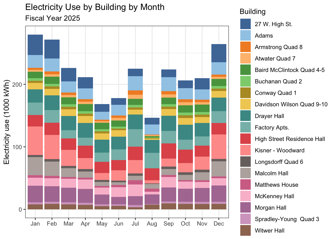
| Version | Author | Date |
|---|---|---|
| 38132bb | maggiedouglas | 2026-03-11 |
Option 2 - faceted, Y axis constant
ggplot(daily_large_res, aes(x= month, y= kwh/(10^3), fill = NAME)) +
  geom_col(position = "stack") +
  facet_wrap(. ~ NAME) +
  scale_fill_paletteer_d("ggthemes::Tableau_20")+
  theme_bw() +
  theme(axis.text.x = element_text(angle = 90, hjust = 1)) +
  theme(legend.position = "none") +
  labs(x = "",
       y = "Electricity use (1000 kWh)",
       title = "Electricity Use by Building by Month",
       subtitle = "Fiscal Year 2025")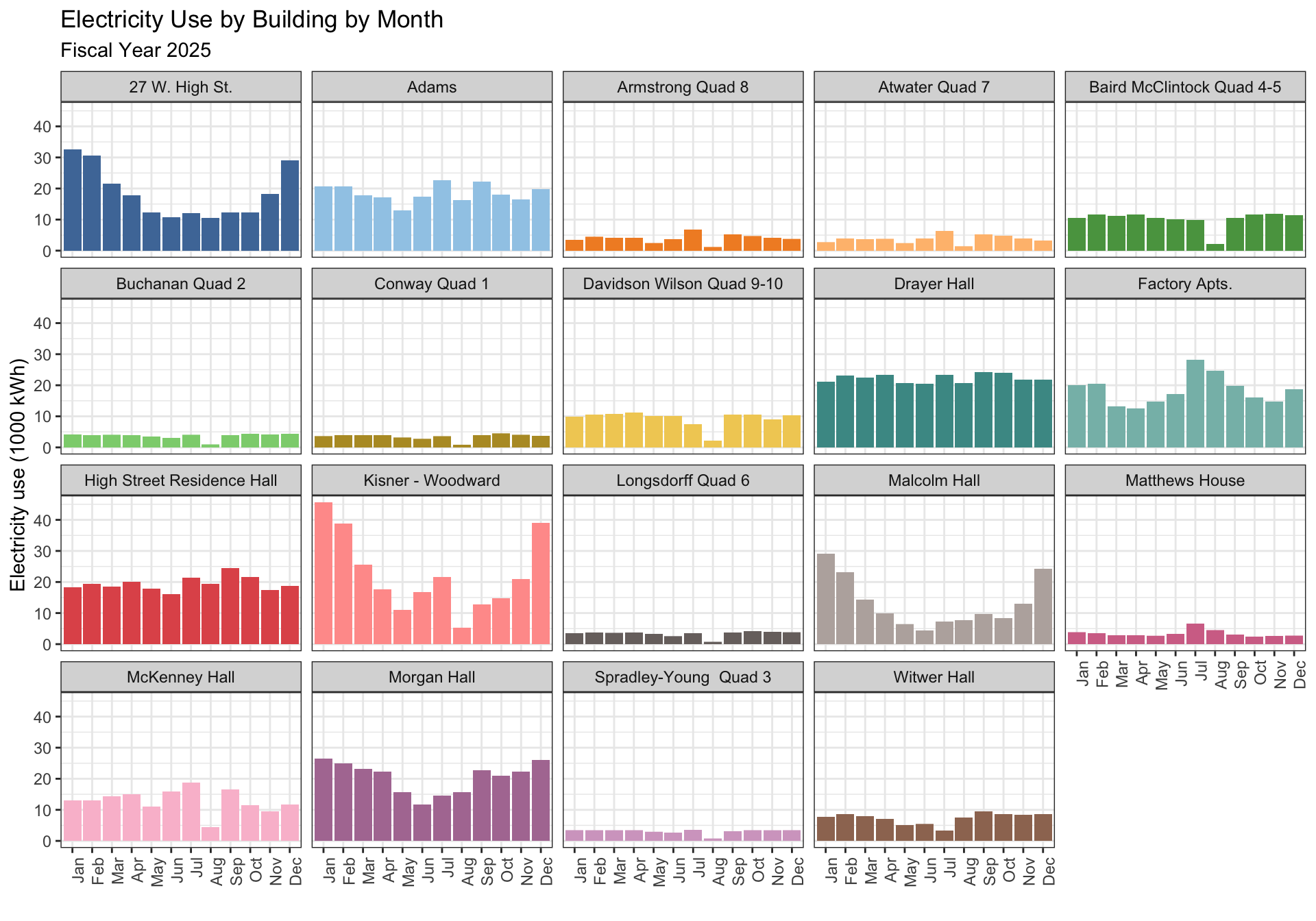
| Version | Author | Date |
|---|---|---|
| 0a9f663 | maggiedouglas | 2026-03-11 |
Option 3 - faceted, Y axis varies
ggplot(daily_large_res, aes(x= month, y= kwh/(10^3), fill = NAME)) +
  geom_col(position = "stack") +
  facet_wrap(. ~ NAME, scales = "free_y") +
  scale_fill_paletteer_d("ggthemes::Tableau_20")+
  theme_bw() +
  theme(axis.text.x = element_text(angle = 90, hjust = 1)) +
  theme(legend.position = "none") +
  labs(x = "",
       y = "Electricity use (1000 kWh)",
       title = "Electricity Use by Building by Month",
       subtitle = "Fiscal Year 2025")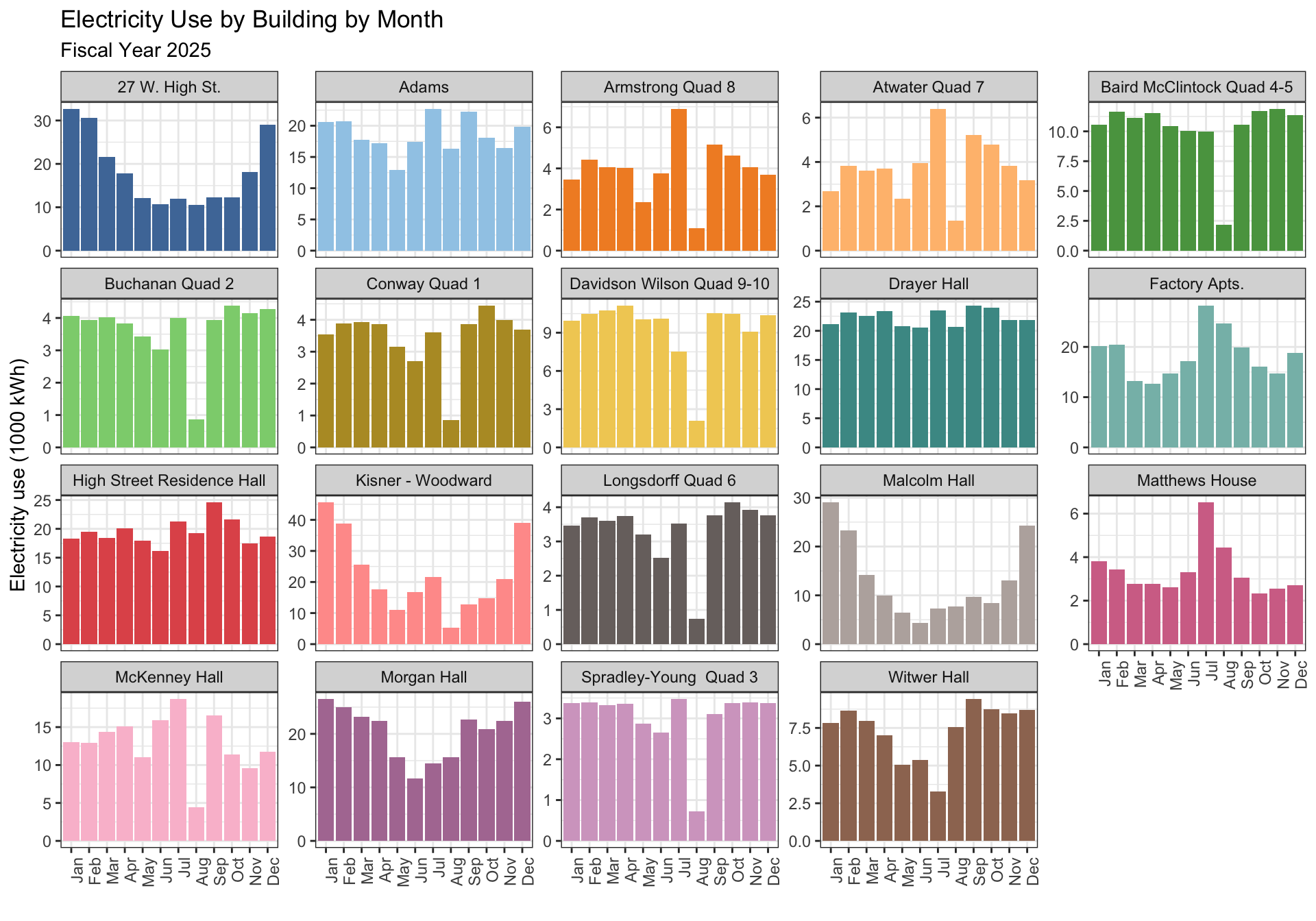
| Version | Author | Date |
|---|---|---|
| 0a9f663 | maggiedouglas | 2026-03-11 |
Electricity intensity
Option 1 - all days included
ggplot(daily_large_res, aes(fct_reorder(NAME, kwh_sqft, median), y = kwh_sqft,
                            fill = NAME)) +
  annotate("rect", xmin=-Inf, xmax=Inf, ymin=8.2, ymax=36.1,
           color="lightgrey", alpha= 0.3) +
  geom_hline(yintercept=13.6, linetype="dashed", color="white") +
  geom_boxplot() +
 # ylim(0,50) +
  theme_bw() +
  theme(legend.position = "none") +
  scale_fill_paletteer_d("ggthemes::Tableau_20") +
  labs(x = "",
       y = "Electricity Intensity (kWh/sqft/year)",
       title = "Electricity Intensity by Square Foot (kWh/sqft/year)") +
  coord_flip()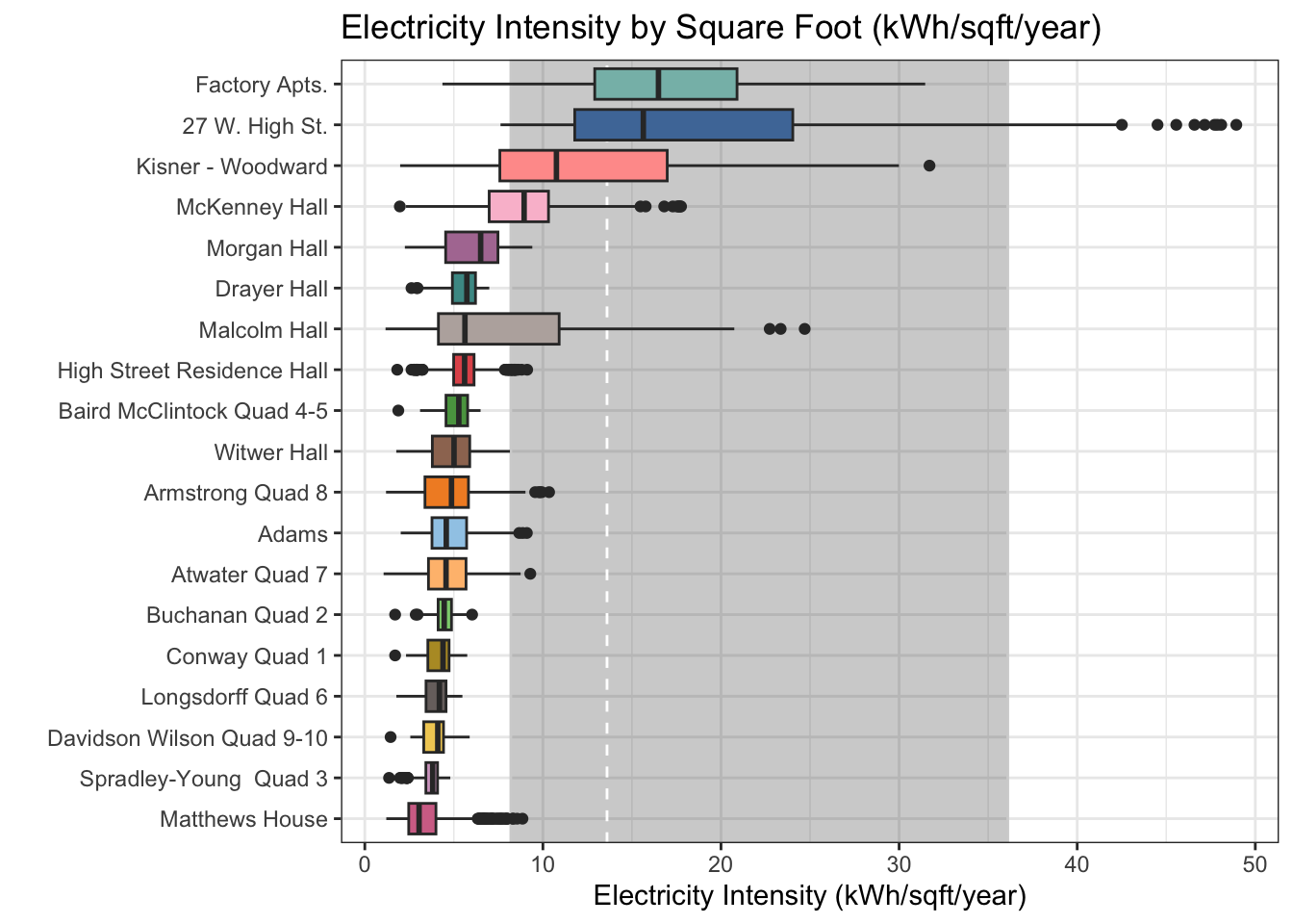
| Version | Author | Date |
|---|---|---|
| 38132bb | maggiedouglas | 2026-03-11 |
Option 2 - only Academic Year
daily_ay <- filter(daily_large_res, period %in% c("Spring","Fall"))

ggplot(daily_ay, aes(fct_reorder(NAME, kwh_sqft, median), y = kwh_sqft,
                            fill = NAME)) +
  annotate("rect", xmin=-Inf, xmax=Inf, ymin=8.2, ymax=36.1,
           color="lightgrey", alpha= 0.3) +
  geom_hline(yintercept=13.6, linetype="dashed", color="white") +
  geom_boxplot() +
#  ylim(0,50) +
  theme_bw() +
  theme(legend.position = "none") +
  scale_fill_paletteer_d("ggthemes::Tableau_20") +
  labs(x = "",
       y = "Electricity Intensity (kWh/sqft/year)",
       title = "Electricity Intensity by Square Foot (kWh/sqft/year)") +
  coord_flip()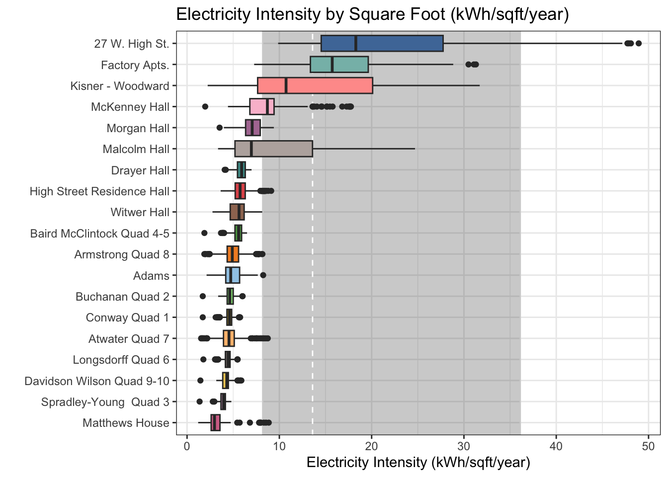
Option 3 - faceted by time of year
daily_large_res$period <- factor(daily_large_res$period,
                                 levels = c("Fall","Spring","Winter","Summer"),
                                 labels = c("Fall Semester","Spring Semester",
                                            "Winter Break","Summer Break"))

ggplot(daily_large_res, aes(fct_reorder(NAME, kwh_sqft, median), y = kwh_sqft,
                            fill = NAME)) +
  annotate("rect", xmin=-Inf, xmax=Inf, ymin=8.2, ymax=36.1,
           color="lightgrey", alpha= 0.3) +
  geom_hline(yintercept=13.6, linetype="dashed", color="white") +
  geom_boxplot() +
  facet_wrap(. ~ period) +
#  ylim(0,50) +
  theme_bw() +
  theme(legend.position = "none") +
  scale_fill_paletteer_d("ggthemes::Tableau_20") +
  labs(x = "",
       y = "Electricity Intensity (kWh/sqft/year)",
       title = "Electricity Intensity by Square Foot (kWh/sqft/year)") +
  coord_flip()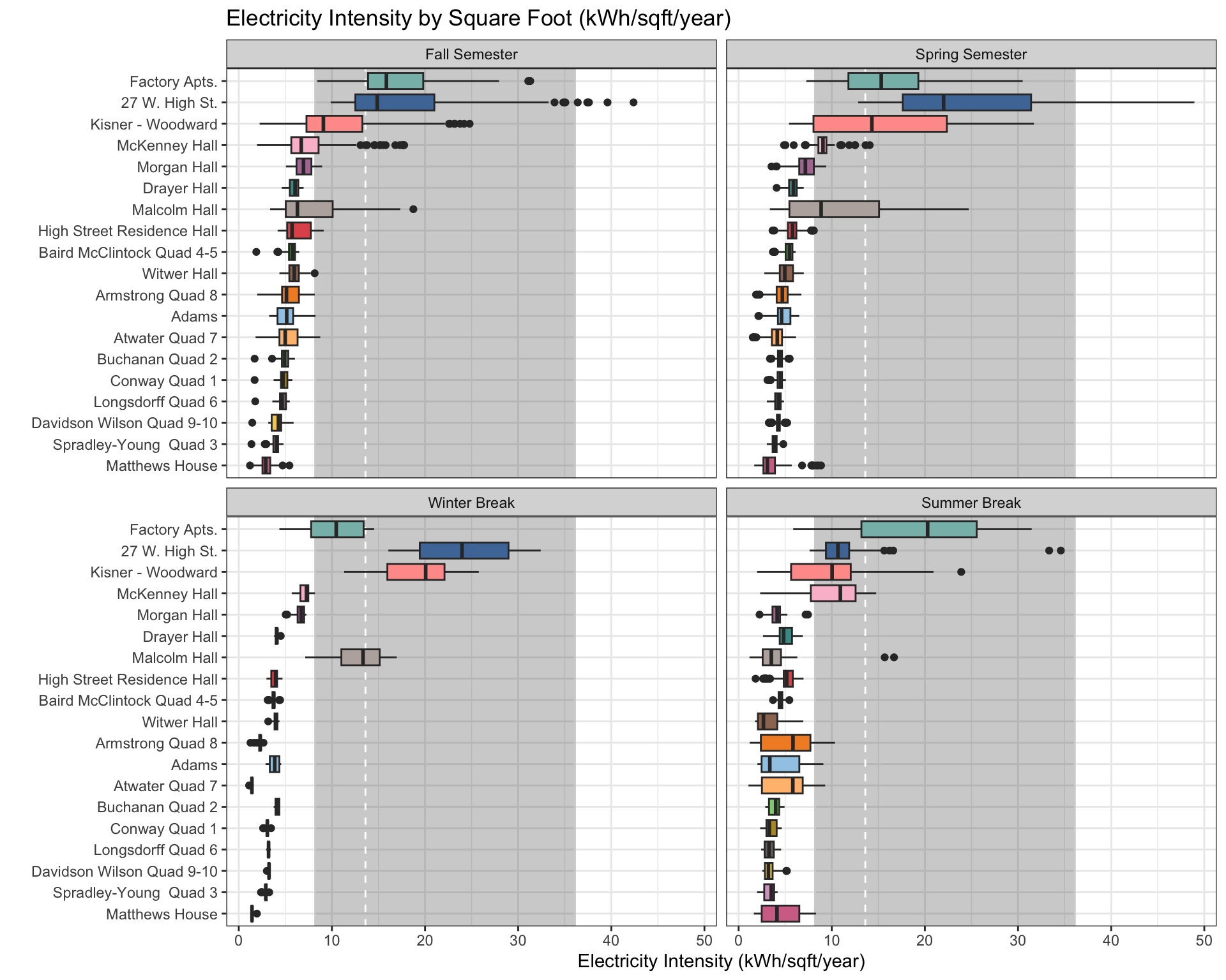
Partner contributions
Claire:
- Worked on the annual electricity data
- Made the summary datatable
- Wrote the partner contributions
Liv:
- Worked on the daily electricity data
- Made the graphs
Data Issues:
There are periods of time when a building meter goes offline, leading to a lot of NA values, then a very high value when the building comes back online. For now, we are adjusting the x-axis limit of the graph to better show the difference between buildings. Note that this means we have removed a lot of the outliers. Other than that, there were no issues.
sessionInfo()R version 4.5.2 (2025-10-31)
Platform: x86_64-apple-darwin20
Running under: macOS Ventura 13.7.8
Matrix products: default
BLAS: /Library/Frameworks/R.framework/Versions/4.5-x86_64/Resources/lib/libRblas.0.dylib
LAPACK: /Library/Frameworks/R.framework/Versions/4.5-x86_64/Resources/lib/libRlapack.dylib; LAPACK version 3.12.1
locale:
[1] en_US.UTF-8/en_US.UTF-8/en_US.UTF-8/C/en_US.UTF-8/en_US.UTF-8
time zone: America/New_York
tzcode source: internal
attached base packages:
[1] stats graphics grDevices utils datasets methods base
other attached packages:
[1] paletteer_1.7.0 DT_0.34.0 lubridate_1.9.5 forcats_1.0.1
[5] stringr_1.6.0 dplyr_1.2.0 purrr_1.2.1 readr_2.2.0
[9] tidyr_1.3.2 tibble_3.3.1 ggplot2_4.0.2 tidyverse_2.0.0
loaded via a namespace (and not attached):
[1] sass_0.4.10 generics_0.1.4 prismatic_1.1.2 stringi_1.8.7
[5] hms_1.1.4 digest_0.6.39 magrittr_2.0.4 timechange_0.4.0
[9] evaluate_1.0.5 grid_4.5.2 RColorBrewer_1.1-3 fastmap_1.2.0
[13] rprojroot_2.1.1 workflowr_1.7.2 jsonlite_2.0.0 whisker_0.4.1
[17] rematch2_2.1.2 promises_1.5.0 crosstalk_1.2.2 scales_1.4.0
[21] jquerylib_0.1.4 cli_3.6.5 rlang_1.1.7 withr_3.0.2
[25] cachem_1.1.0 yaml_2.3.12 otel_0.2.0 tools_4.5.2
[29] tzdb_0.5.0 httpuv_1.6.16 vctrs_0.7.1 R6_2.6.1
[33] lifecycle_1.0.5 git2r_0.36.2 htmlwidgets_1.6.4 fs_1.6.7
[37] pkgconfig_2.0.3 pillar_1.11.1 bslib_0.10.0 later_1.4.8
[41] gtable_0.3.6 glue_1.8.0 Rcpp_1.1.1 xfun_0.56
[45] tidyselect_1.2.1 rstudioapi_0.18.0 knitr_1.51 farver_2.1.2
[49] htmltools_0.5.9 labeling_0.4.3 rmarkdown_2.30 compiler_4.5.2
[53] S7_0.2.1