Simulations with UK Biobank genotypes and different effect structure across traits
Fabio Morgante & Deborah Kunkel
October 21, 2023
Last updated: 2023-10-21
Checks: 7 0
Knit directory: mr_mash_rss/
This reproducible R Markdown analysis was created with workflowr (version 1.7.0). The Checks tab describes the reproducibility checks that were applied when the results were created. The Past versions tab lists the development history.
Great! Since the R Markdown file has been committed to the Git repository, you know the exact version of the code that produced these results.
Great job! The global environment was empty. Objects defined in the global environment can affect the analysis in your R Markdown file in unknown ways. For reproduciblity it’s best to always run the code in an empty environment.
The command set.seed(20230612) was run prior to running
the code in the R Markdown file. Setting a seed ensures that any results
that rely on randomness, e.g. subsampling or permutations, are
reproducible.
Great job! Recording the operating system, R version, and package versions is critical for reproducibility.
Nice! There were no cached chunks for this analysis, so you can be confident that you successfully produced the results during this run.
Great job! Using relative paths to the files within your workflowr project makes it easier to run your code on other machines.
Great! You are using Git for version control. Tracking code development and connecting the code version to the results is critical for reproducibility.
The results in this page were generated with repository version e0b7f14. See the Past versions tab to see a history of the changes made to the R Markdown and HTML files.
Note that you need to be careful to ensure that all relevant files for
the analysis have been committed to Git prior to generating the results
(you can use wflow_publish or
wflow_git_commit). workflowr only checks the R Markdown
file, but you know if there are other scripts or data files that it
depends on. Below is the status of the Git repository when the results
were generated:
Ignored files:
    Ignored:    .snakemake/
    Ignored:    data/
    Ignored:    output/
    Ignored:    run/
    Ignored:    tmp/

Untracked files:
    Untracked:  Snakefile_old
    Untracked:  analysis/ukb_bc_results.Rmd
    Untracked:  code/adjust_LD_test.R
    Untracked:  code/compute_sumstats_test_bc_ukb.R
    Untracked:  code/fit_kriging_rss_ukb.R
    Untracked:  code/fit_mrmashrss_test_ukb.R
    Untracked:  code/merge_sumstats_all_chr_ukb.R
    Untracked:  code/split_effects_by_chr_imp_ukb.R
    Untracked:  scripts/11_run_fit_mrmashrss_by_chr_V_all_chr_bc_ukb.sbatch
    Untracked:  scripts/11_run_fit_mrmashrss_sparse_LD_V_all_chr_by_chr_bc_ukb.sbatch
    Untracked:  scripts/11_run_fit_mrmashrss_sparse_LD_mvsusie_paper_prior_by_chr_bc_ukb.sbatch
    Untracked:  scripts/11_run_fit_mrmashrss_test_by_chr_V_all_chr_bc_ukb.sbatch
    Untracked:  scripts/12_run_compute_pred_accuracy_mrmashrss_sparse_LD_V_all_chr_bc_ukb.sbatch
    Untracked:  scripts/12_run_compute_pred_accuracy_mrmashrss_sparse_LD_mvsusie_paper_prior_bc_ukb.sbatch
    Untracked:  scripts/3_run_compute_sumstats_by_chr_and_fold_test_bc_ukb.sbatch
    Untracked:  scripts/run_adjust_LD_test.sbatch
    Untracked:  scripts/run_fit_kriging_rss_by_chr_and_trait_bc_ukb.sbatch

Unstaged changes:
    Modified:   code/compute_prediction_accuracy_bc_ukb.R
    Modified:   ukb_sim_snakemake_submitter.sh
Note that any generated files, e.g. HTML, png, CSS, etc., are not included in this status report because it is ok for generated content to have uncommitted changes.
These are the previous versions of the repository in which changes were
made to the R Markdown (analysis/ukb_sim_results.Rmd) and
HTML (docs/ukb_sim_results.html) files. If you’ve
configured a remote Git repository (see ?wflow_git_remote),
click on the hyperlinks in the table below to view the files as they
were in that past version.
| File | Version | Author | Date | Message |
|---|---|---|---|---|
| html | e0b7f14 | fmorgante | 2023-10-20 | Build site. |
| html | eb09d7b | fmorgante | 2023-10-19 | Build site. |
| html | e8a2096 | fmorgante | 2023-10-18 | Build site. |
| Rmd | 2e7c7bd | fmorgante | 2023-10-18 | Update equal effects results |
| Rmd | 68bbbfc | fmorgante | 2023-10-02 | Minor changes |
| html | b5ea188 | fmorgante | 2023-08-04 | Build site. |
| Rmd | 324f45d | fmorgante | 2023-08-04 | Fix typo |
| html | 70e6d4a | fmorgante | 2023-08-04 | Build site. |
| Rmd | 1748dc9 | fmorgante | 2023-08-04 | Fix interpretation and graph |
| html | f38634b | fmorgante | 2023-08-04 | Build site. |
| Rmd | 7460ddc | fmorgante | 2023-08-04 | Add more polygenic scenario |
| html | a826a15 | fmorgante | 2023-07-31 | Build site. |
| Rmd | f0e1213 | fmorgante | 2023-07-31 | Add filtered plots |
| html | aa87dd0 | fmorgante | 2023-07-31 | Build site. |
| Rmd | 7c91a7c | fmorgante | 2023-07-31 | Fix bug |
| html | 33d8243 | fmorgante | 2023-07-31 | Build site. |
| Rmd | 31759a7 | fmorgante | 2023-07-31 | Add low PVE and 10 traits scenarios |
| html | 7b4d53c | fmorgante | 2023-07-31 | Build site. |
| Rmd | 36c46c0 | fmorgante | 2023-07-31 | Add bayesR |
| html | 9d82631 | fmorgante | 2023-06-28 | Build site. |
| Rmd | c34b451 | fmorgante | 2023-06-28 | Fix number |
| html | fd5c2b8 | fmorgante | 2023-06-28 | Build site. |
| Rmd | 84a9e87 | fmorgante | 2023-06-28 | Fix wording again |
| html | 8e716cf | fmorgante | 2023-06-28 | Build site. |
| Rmd | 21fdce5 | fmorgante | 2023-06-28 | Fix wording |
| html | ed4d773 | fmorgante | 2023-06-28 | Build site. |
| Rmd | 1b792ed | fmorgante | 2023-06-28 | Add a few more details |
| html | 3da045b | fmorgante | 2023-06-28 | Build site. |
| Rmd | 963fdb6 | fmorgante | 2023-06-28 | Add shared in subgroups scenario |
| html | 6469c43 | fmorgante | 2023-06-22 | Build site. |
| Rmd | 6327343 | fmorgante | 2023-06-22 | Minor change |
| html | 033b736 | fmorgante | 2023-06-22 | Build site. |
| Rmd | ee36241 | fmorgante | 2023-06-22 | Add mostly null scenario |
| html | 42fe7e0 | fmorgante | 2023-06-13 | Build site. |
| Rmd | 67a6127 | fmorgante | 2023-06-13 | Add another clarification |
| html | 1b1f3d6 | fmorgante | 2023-06-13 | Build site. |
| Rmd | d47b9bc | fmorgante | 2023-06-13 | Add clarification |
| html | 383a73f | fmorgante | 2023-06-13 | Build site. |
| Rmd | 3ecaea0 | fmorgante | 2023-06-13 | Minor improvements 2.0 |
| html | 9291d6d | fmorgante | 2023-06-13 | Build site. |
| Rmd | dad6412 | fmorgante | 2023-06-13 | Minor improvements |
| html | b4baad5 | fmorgante | 2023-06-13 | Build site. |
| Rmd | a222e7b | fmorgante | 2023-06-13 | Add more details |
| html | 409ae91 | fmorgante | 2023-06-12 | Build site. |
| Rmd | e56eb43 | fmorgante | 2023-06-12 | workflowr::wflow_publish("analysis/ukb_sim_results.Rmd") |
| html | 886b637 | fmorgante | 2023-06-12 | Build site. |
| Rmd | 2df5821 | fmorgante | 2023-06-12 | wflow_publish("analysis/ukb_sim_results.Rmd") |
###Load libraries
library(ggplot2)
library(cowplot)

repz <- 1:20
prefix <- "output/prediction_accuracy/ukb_caucasian_white_british_unrel_100000"
metric <- "r2"
traitz <- 1:5
Introduction
The goal of this analysis is to benchmark the newly developed mr.mash.rss (aka mr.mash with summary data) against already existing methods in the task of predicting phenotypes from genotypes using only summary data. To do so, we used real genotypes from the array data of the UK Biobank. We randomly sampled 105,000 nominally unrelated (\(r_A\) < 0.025 between any pair) individuals of European ancestry (i.e., Caucasian and white British fields). After retaining variants with minor allele frequency (MAF) > 0.01, minor allele count (MAC) > 5, genotype missing rate < 0.1 and Hardy-Weinberg Equilibrium (HWE) test p-value > \(1 *10^{-10}\), our data consisted of 595,071 genetic variants (i.e., our predictors). Missing genotypes were imputed with the mean genotype for the respective genetic variant.
The linkage disequilibrium (LD) matrices (i.e., the correlation matrices) were computed using 146,288 nominally unrelated (\(r_A\) < 0.025 between any pair) individuals of European ancestry (i.e., Caucasian and white British fields), that did not overlap with the 105,000 individuals used for the rest of the analyses.
For each replicate, we simulated 5 traits (i.e., our responses) by randomly sampling 5,000 variants (out of the total of 595,071) to be causal, with different effect sharing structures across traits (see below). The genetic effects explain 50% of the total per-trait variance (except for two scenario as explained below) – in genetics terminology this is called genomic heritability (\(h_g^2\)). The residuals are uncorrelated across traits.
We randomly sampled 5,000 (out of the 105,000) individuals to be the test set. The test set was only used to evaluate prediction accuracy. All the other steps were carried out on the training set of 100,000 individuals.
Summary statistics (i.e., effect size and its standard error) were obtained by univariate simple linear regression of each trait on each variant, one at a time. Traits and variants were not standardized.
Four different methods were fitted:
- LDpred2 per-chromosome with the auto option, 500 iterations (after 500 burn-in iterations), \(h^2\) initialized as 0.5/22 and \(p\) initialized using the same grid as in the original paper. NB this is a univariate method.
- LDpred2 genome-wide with the auto option, 500 iterations (after 500 burn-in iterations), \(h^2\) initialized as 0.5/22 (WRONG) and \(p\) initialized using the same grid as in the original paper. NB this is a univariate method.
- mr.mash.rss per-chromosome, with both canonical and data-driven covariance matrices computed as described in the mr.mash paper, updating the (full rank) residual covariance and the mixture weights, without standardizing the variables. The residual covariance was initialized as in the mvSuSiE paper and the mixture weights were initialized as 90% of the weight on the null component and 10% of the weight split equally across the remaining components. The phenotypic covariance was computed as the sample covariance using the individual-level data. NB this is a multivariate method.
- BayesR per-chromosome, with 1000 iterations (after 500 burn-in iterations), \(h^2\) initialized as 0.5/22 and other default parameters. NB this is a univariate method. We used the implementation in the qgg R package.
Prediction accuracy was evaluated as the \(R^2\) of the regression of true phenotypes on the predicted phenotypes. This metric as the attractive property that its upper bound is \(h_g^2\).
20 replicates for each simulation scenario were run.
Equal effects scenario
In this scenario, the effects were drawn from a Multivariate Normal distribution with mean vector 0 and covariance matrix that achieves a per-trait variance of 1 and a correlation across traits of 1. This implies that the effects of the causal variants are equal across responses.
scenarioz <- "equal_effects_indep_resid"
methodz <- c("mr_mash_rss", "ldpred2_auto")#, "ldpred2_auto_gwide", "bayesR")

i <- 0

n_col <- 6
n_row <- length(repz) * length(scenarioz) * length(methodz) * length(traitz)
res <- as.data.frame(matrix(NA, ncol=n_col, nrow=n_row))
colnames(res) <- c("rep", "scenario", "method", "trait", "metric", "score")

for(sce in scenarioz){
  for(met in methodz){
    for(repp in repz){
      dat <- readRDS(paste0(prefix, "_", sce, "_", met, "_pred_acc_", repp, ".rds"))

      for(trait in traitz){
        i <- i + 1

        res[i, 1] <- repp
        res[i, 2] <- sce
        res[i, 3] <- met
        res[i, 4] <- trait
        res[i, 5] <- metric
        res[i, 6] <- dat$r2[trait]
      }
    }
  }
}

res <- transform(res, scenario=as.factor(scenario),
                      method=as.factor(method),
                      trait=as.factor(trait))

p_methods_shared <- ggplot(res, aes(x = trait, y = score, fill = method)) +
  geom_boxplot(color = "black", outlier.size = 1, width = 0.85) +
  stat_summary(fun=mean, geom="point", shape=23,
               position = position_dodge2(width = 0.87,
                                          preserve = "single")) +
  ylim(0, 0.51) +
  scale_fill_manual(values = c("pink", "red", "green", "blue")) +
  labs(x = "Trait", y = expression(italic(R)^2), fill="Method", title="") +
  geom_hline(yintercept=0.5, linetype="dotted", linewidth=1, color = "black") +
  theme_cowplot(font_size = 18)

print(p_methods_shared)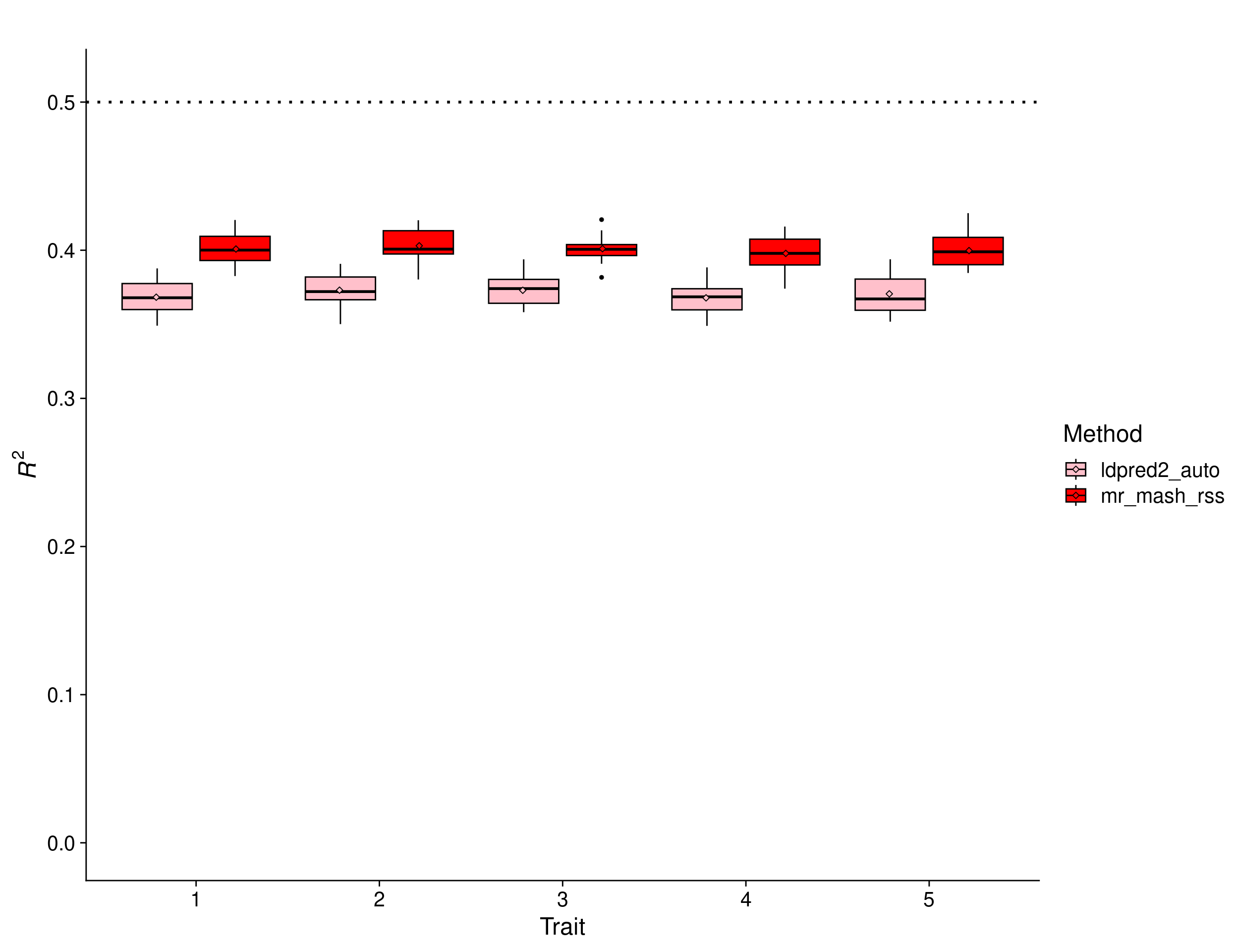
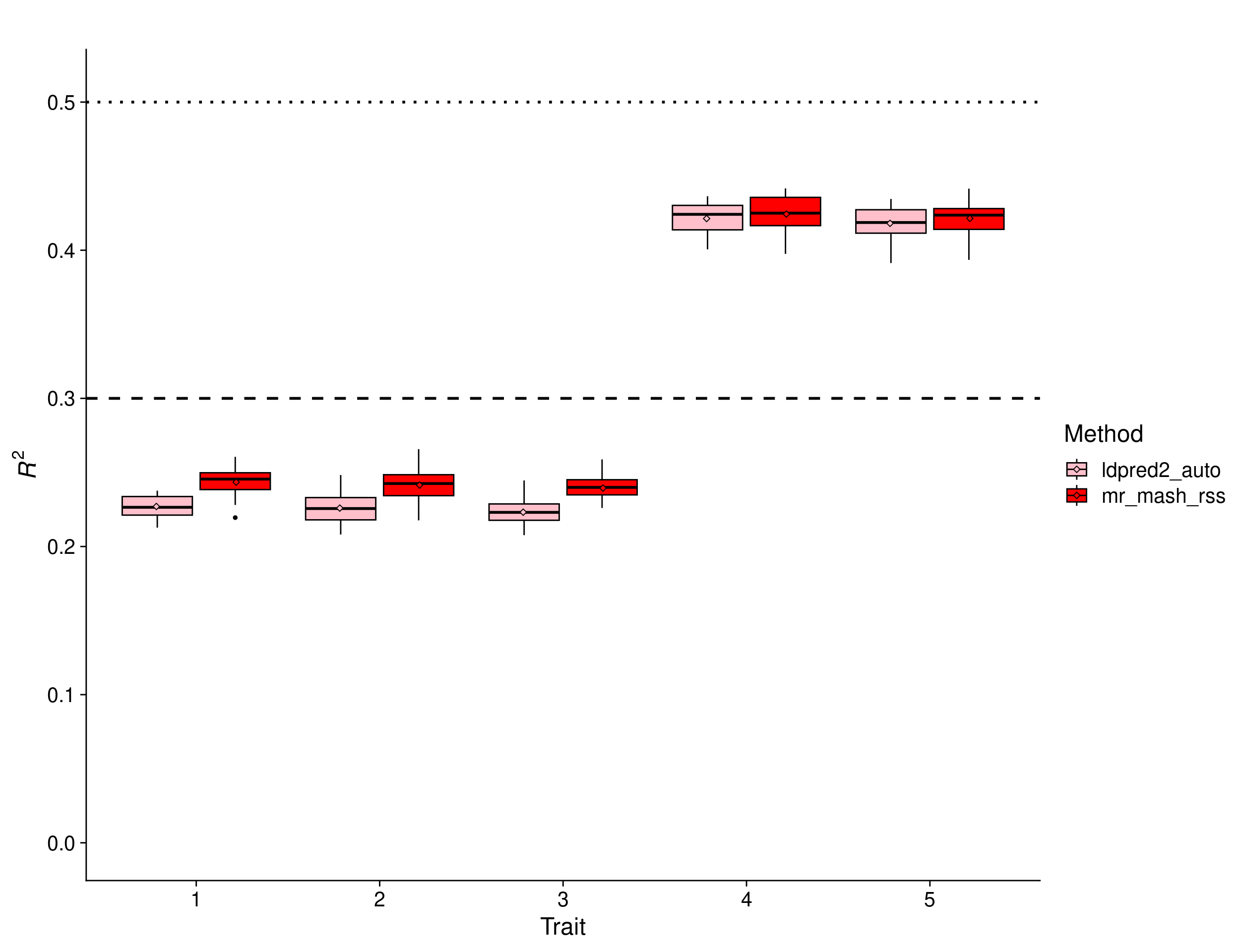
In this scenario, there is a clear advantage to using multivariate methods. In fact, given that the effects are equal across traits and the residuals are uncorrelated, a multivariate analysis is roughly equivalent to having 5 times as many samples as in an univariate analysis. The results show that mr.mash.rss clearly does better than both flavors of LDpred2 auto. However, in this simulation there does not seem to be much of a difference between LDpred2 auto per-chromosome and genome-wide. Therefore, we will drop LDpred2 auto genome-wide from further analyses since it is more computationally intensive. BayesR gives unreasonably low prediction accuracy, which hints at issues with the default parameters and/or this particular implementation.
Mostly null scenario
In this scenario, the effects were drawn from a Multivariate Normal distribution with mean vector 0 and covariance matrix that achieves effects (with variance 1) to be present only trait 1. The other 4 traits are only random noise.
scenarioz <- "trait_1_only_effects_indep_resid"
methodz <- c("mr_mash_rss", "ldpred2_auto")#, "bayesR")

i <- 0

n_col <- 6
n_row <- length(repz) * length(scenarioz) * length(methodz) * length(traitz)
res <- as.data.frame(matrix(NA, ncol=n_col, nrow=n_row))
colnames(res) <- c("rep", "scenario", "method", "trait", "metric", "score")

for(sce in scenarioz){
  for(met in methodz){
    for(repp in repz){
      dat <- readRDS(paste0(prefix, "_", sce, "_", met, "_pred_acc_", repp, ".rds"))

      for(trait in traitz){
        i <- i + 1

        res[i, 1] <- repp
        res[i, 2] <- sce
        res[i, 3] <- met
        res[i, 4] <- trait
        res[i, 5] <- metric
        res[i, 6] <- dat$r2[trait]
      }
    }
  }
}

res <- transform(res, scenario=as.factor(scenario),
                      method=as.factor(method),
                      trait=as.factor(trait))

p_mostly_null <- ggplot(res, aes(x = trait, y = score, fill = method)) +
  geom_boxplot(color = "black", outlier.size = 1, width = 0.85) +
  stat_summary(fun=mean, geom="point", shape=23,
               position = position_dodge2(width = 0.87,
                                          preserve = "single")) +
  ylim(0.0, 0.51) +
  scale_fill_manual(values = c("pink", "red", "blue")) +
  labs(x = "Trait", y = expression(italic(R)^2), fill="Method", title="") +
  geom_hline(yintercept=0.5, linetype="dotted", linewidth=1, color = "black") +
  theme_cowplot(font_size = 18)

print(p_mostly_null)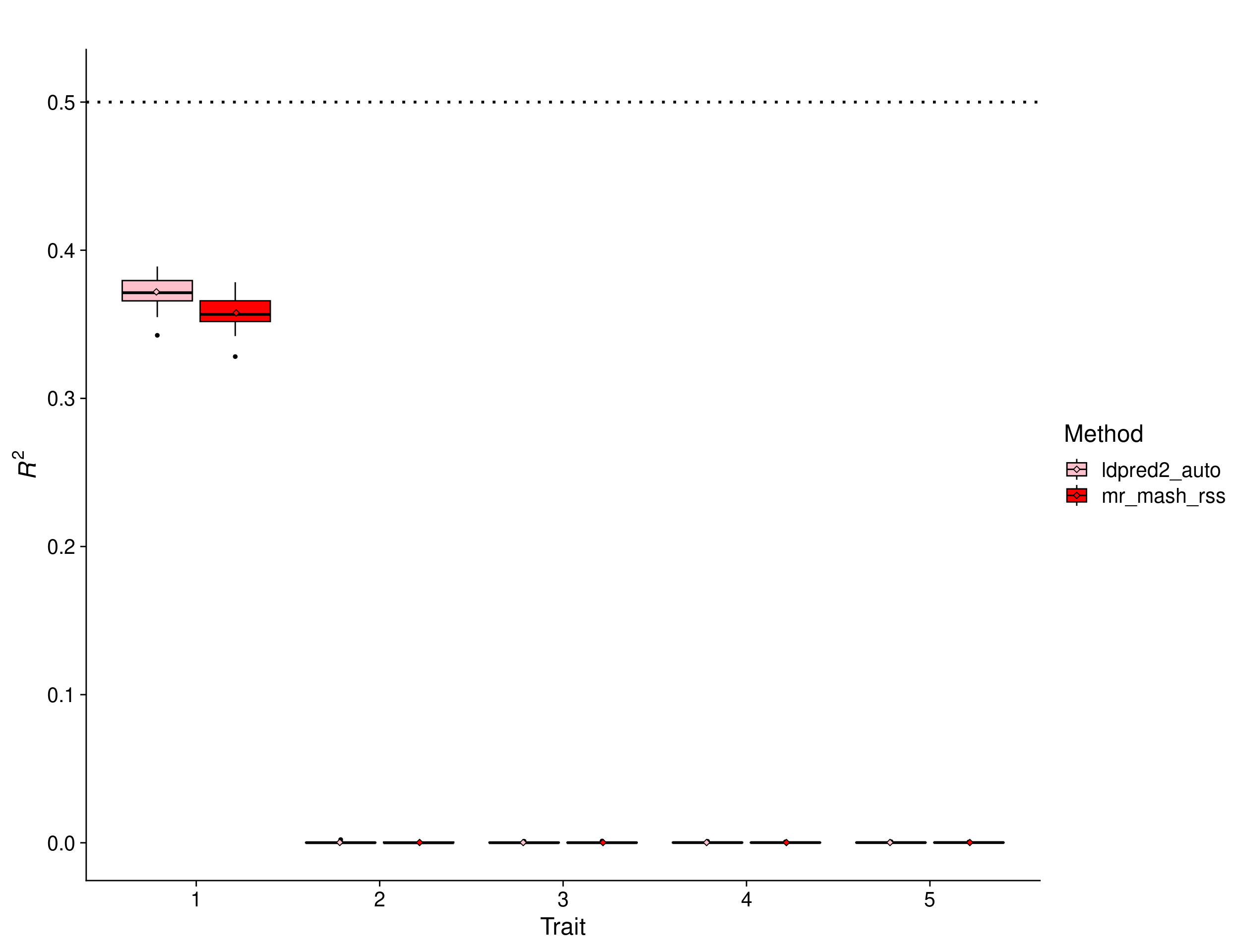
In this scenario, there is no advantage to using multivariate methods. In fact, there is potential for multivariate methods to do worse than univariate methods because of the large amount of noise modeled jointly with the signal. However, the results show that mr.mash.rss can learn this structure from the data and, reassuringly, performs similarly to LDpred2 auto. Again, **BayesR* gives unreasonably low prediction accuracy, which hints at issues with the default parameters and/or this particular implementation.
Equal effects scenario – low PVE
In this scenario, the effects were drawn from a Multivariate Normal distribution with mean vector 0 and covariance matrix that achieves a per-trait variance of 1 and a correlation across traits of 1. This implies that the effects of the causal variants are equal across responses. In addition, the per-trait genomic heritability was set to 0.2.
scenarioz <- "equal_effects_low_pve_indep_resid"
methodz <- c("mr_mash_rss", "ldpred2_auto")#, "bayesR")

i <- 0

n_col <- 6
n_row <- length(repz) * length(scenarioz) * length(methodz) * length(traitz)
res <- as.data.frame(matrix(NA, ncol=n_col, nrow=n_row))
colnames(res) <- c("rep", "scenario", "method", "trait", "metric", "score")

for(sce in scenarioz){
  for(met in methodz){
    for(repp in repz){
      dat <- readRDS(paste0(prefix, "_", sce, "_", met, "_pred_acc_", repp, ".rds"))

      for(trait in traitz){
        i <- i + 1

        res[i, 1] <- repp
        res[i, 2] <- sce
        res[i, 3] <- met
        res[i, 4] <- trait
        res[i, 5] <- metric
        res[i, 6] <- dat$r2[trait]
      }
    }
  }
}

res <- transform(res, scenario=as.factor(scenario),
                      method=as.factor(method),
                      trait=as.factor(trait))

p_methods_shared_lowpve <- ggplot(res, aes(x = trait, y = score, fill = method)) +
  geom_boxplot(color = "black", outlier.size = 1, width = 0.85) +
  stat_summary(fun=mean, geom="point", shape=23,
               position = position_dodge2(width = 0.87,
                                          preserve = "single")) +
  ylim(0, 0.2) +
  scale_fill_manual(values = c("pink", "red", "blue")) +
  labs(x = "Trait", y = expression(italic(R)^2), fill="Method", title="") +
  geom_hline(yintercept=0.2, linetype="dotted", linewidth=1, color = "black") +
  theme_cowplot(font_size = 18)

print(p_methods_shared_lowpve)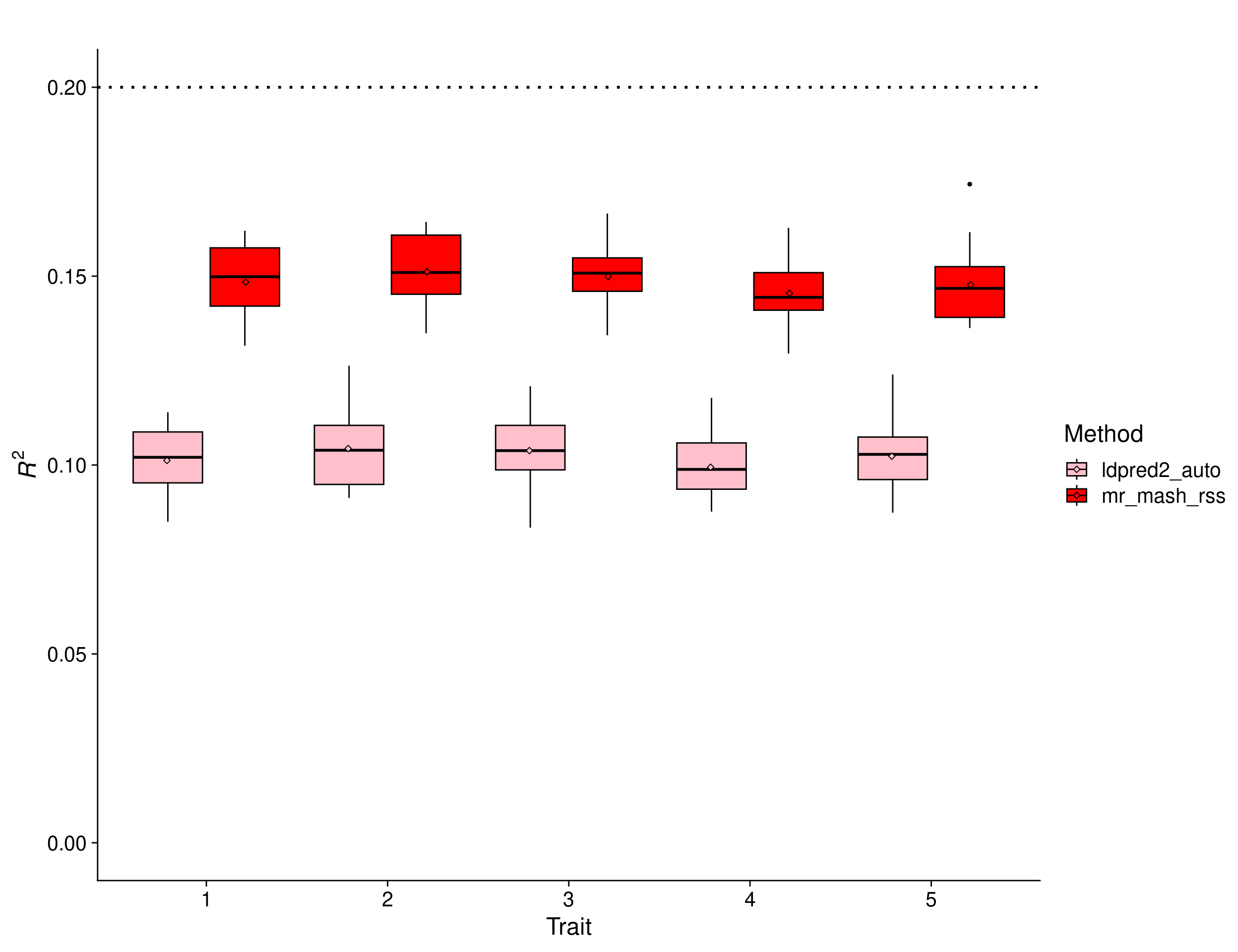
In this scenario, we expect the relative improvement of multivariate methods compared to univariate methods to be larger than with \(h^2_g = 0.5\). This is because with smaller signal-to-noise ratio, it is harder for univariate methods to estimate effects accurately. Multivariate methods can borrow information across traits (if effects are shared) and improve accuracy. The results show that mr.mash.rss clearly does better than LDpred2 auto. Again, BayesR gives unreasonably low prediction accuracy, which hints at issues with the default parameters and/or this particular implementation.
Equal effects scenario – more polygenic
In this scenario, the effects were drawn from a Multivariate Normal distribution with mean vector 0 and covariance matrix that achieves a per-trait variance of 1 and a correlation across traits of 1. This implies that the effects of the causal variants are equal across responses. In addition, the number of causal variants was set to 50,000.
scenarioz <- "equal_effects_50000causal_indep_resid"
methodz <- c("mr_mash_rss", "ldpred2_auto")

i <- 0

n_col <- 6
n_row <- length(repz) * length(scenarioz) * length(methodz) * length(traitz)
res <- as.data.frame(matrix(NA, ncol=n_col, nrow=n_row))
colnames(res) <- c("rep", "scenario", "method", "trait", "metric", "score")

for(sce in scenarioz){
  for(met in methodz){
    for(repp in repz){
      dat <- readRDS(paste0(prefix, "_", sce, "_", met, "_pred_acc_", repp, ".rds"))

      for(trait in traitz){
        i <- i + 1

        res[i, 1] <- repp
        res[i, 2] <- sce
        res[i, 3] <- met
        res[i, 4] <- trait
        res[i, 5] <- metric
        res[i, 6] <- dat$r2[trait]
      }
    }
  }
}

res <- transform(res, scenario=as.factor(scenario),
                      method=as.factor(method),
                      trait=as.factor(trait))

p_methods_shared_lowpve <- ggplot(res, aes(x = trait, y = score, fill = method)) +
  geom_boxplot(color = "black", outlier.size = 1, width = 0.85) +
  stat_summary(fun=mean, geom="point", shape=23,
               position = position_dodge2(width = 0.87,
                                          preserve = "single")) +
  ylim(0, 0.5) +
  scale_fill_manual(values = c("red", "blue")) +
  labs(x = "Trait", y = expression(italic(R)^2), fill="Method", title="") +
  geom_hline(yintercept=0.5, linetype="dotted", linewidth=1, color = "black") +
  theme_cowplot(font_size = 18)

print(p_methods_shared_lowpve)
In this scenario, we expect the accuracy to be lower because of the much larger number of causal variants, each explaining a much lower proportion of the total \(h^2_g=0.5\). Multivariate methods can borrow information across traits (if effects are shared) and improve accuracy. The results show that mr.mash.rss clearly does better than LDpred2 auto in this scenario too.
Equal effects scenario – 10 traits
In this scenario, the effects were drawn from a Multivariate Normal distribution with mean vector 0 and covariance matrix that achieves a per-trait variance of 1 and a correlation across traits of 1. This implies that the effects of the causal variants are equal across responses. In addition, the number of traits was increased to 10.
scenarioz <- "equal_effects_10traits_indep_resid"
methodz <- c("mr_mash_rss", "ldpred2_auto")#, "bayesR")

i <- 0

traitz <- 1:10
repz <- c(1:10, 12:20)

n_col <- 6
n_row <- length(repz) * length(scenarioz) * length(methodz) * length(traitz)
res <- as.data.frame(matrix(NA, ncol=n_col, nrow=n_row))
colnames(res) <- c("rep", "scenario", "method", "trait", "metric", "score")

for(sce in scenarioz){
  for(met in methodz){
    for(repp in repz){
      dat <- readRDS(paste0(prefix, "_", sce, "_", met, "_pred_acc_", repp, ".rds"))

      for(trait in traitz){
        i <- i + 1

        res[i, 1] <- repp
        res[i, 2] <- sce
        res[i, 3] <- met
        res[i, 4] <- trait
        res[i, 5] <- metric
        res[i, 6] <- dat$r2[trait]
      }
    }
  }
}

res <- transform(res, scenario=as.factor(scenario),
                      method=as.factor(method),
                      trait=as.factor(trait))

p_methods_shared_10traits <- ggplot(res, aes(x = trait, y = score, fill = method)) +
  geom_boxplot(color = "black", outlier.size = 1, width = 0.85) +
  stat_summary(fun=mean, geom="point", shape=23,
               position = position_dodge2(width = 0.87,
                                          preserve = "single")) +
  ylim(0, 0.51) +
  scale_fill_manual(values = c("pink", "red", "blue")) +
  labs(x = "Trait", y = expression(italic(R)^2), fill="Method", title="") +
  geom_hline(yintercept=0.5, linetype="dotted", linewidth=1, color = "black") +
  theme_cowplot(font_size = 18)

print(p_methods_shared_10traits)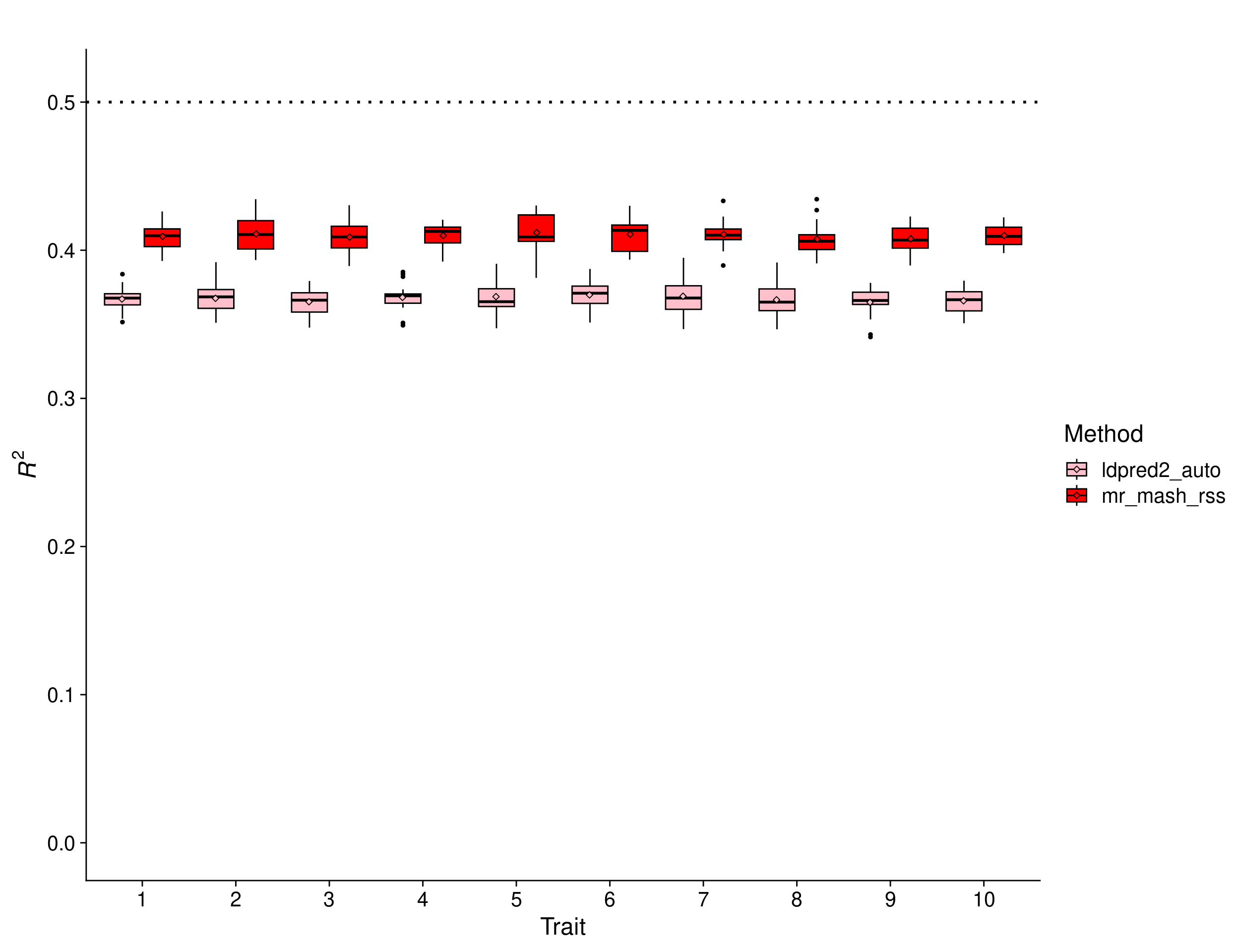
In this scenario, we expect the relative improvement of multivariate methods compared to univariate methods to be a little larger than with 5 traits. This is because multivariate methods can borrow information across a larger number of traits (if effects are shared) and improve accuracy. The results show that mr.mash.rss clearly does better than LDpred2 auto, but the improvement compared to the scenario with 5 traits is small (\(mean(\frac{mr.mash.rss R^2}{LDpred2 auto R^2}) = 1.1157\) vs \(mean(\frac{mr.mash.rss R^2}{LDpred2 auto R^2}) = 1.1057\)). Again, BayesR gives unreasonably low prediction accuracy, which hints at issues with the default parameters and/or this particular implementation.
sessionInfo()R version 4.1.2 (2021-11-01)
Platform: x86_64-pc-linux-gnu (64-bit)
Running under: Rocky Linux 8.5 (Green Obsidian)
Matrix products: default
BLAS/LAPACK: /opt/ohpc/pub/libs/gnu9/openblas/0.3.7/lib/libopenblasp-r0.3.7.so
locale:
[1] LC_CTYPE=en_US.UTF-8 LC_NUMERIC=C
[3] LC_TIME=en_US.UTF-8 LC_COLLATE=en_US.UTF-8
[5] LC_MONETARY=en_US.UTF-8 LC_MESSAGES=en_US.UTF-8
[7] LC_PAPER=en_US.UTF-8 LC_NAME=C
[9] LC_ADDRESS=C LC_TELEPHONE=C
[11] LC_MEASUREMENT=en_US.UTF-8 LC_IDENTIFICATION=C
attached base packages:
[1] stats graphics grDevices utils datasets methods base
other attached packages:
[1] cowplot_1.1.1 ggplot2_3.4.3
loaded via a namespace (and not attached):
[1] Rcpp_1.0.11 highr_0.10 pillar_1.9.0 compiler_4.1.2
[5] bslib_0.5.0 later_1.3.1 jquerylib_0.1.4 git2r_0.32.0
[9] workflowr_1.7.0 tools_4.1.2 digest_0.6.33 gtable_0.3.3
[13] jsonlite_1.8.7 evaluate_0.21 lifecycle_1.0.3 tibble_3.2.1
[17] pkgconfig_2.0.3 rlang_1.1.1 cli_3.6.1 rstudioapi_0.15.0
[21] yaml_2.3.7 xfun_0.39 fastmap_1.1.1 withr_2.5.0
[25] dplyr_1.1.2 stringr_1.5.0 knitr_1.43 generics_0.1.3
[29] fs_1.6.3 vctrs_0.6.3 sass_0.4.7 tidyselect_1.2.0
[33] rprojroot_2.0.3 grid_4.1.2 glue_1.6.2 R6_2.5.1
[37] fansi_1.0.4 rmarkdown_2.23 farver_2.1.1 magrittr_2.0.3
[41] whisker_0.4.1 scales_1.2.1 promises_1.2.0.1 htmltools_0.5.5
[45] colorspace_2.1-0 httpuv_1.6.11 labeling_0.4.2 utf8_1.2.3
[49] stringi_1.7.12 munsell_0.5.0 cachem_1.0.8 