data_analysis_salience

workflowr

• Summary
• Checks
• Past versions

Last updated: 2022-03-01

Checks: 6 1

Knit directory: project_video_salience/

This reproducible R Markdown analysis was created with workflowr (version 1.6.2). The Checks tab describes the reproducibility checks that were applied when the results were created. The Past versions tab lists the development history.

---

R Markdown file: up-to-date

Great! Since the R Markdown file has been committed to the Git repository, you know the exact version of the code that produced these results.

Environment: empty

Great job! The global environment was empty. Objects defined in the global environment can affect the analysis in your R Markdown file in unknown ways. For reproduciblity it’s best to always run the code in an empty environment.

Seed: set.seed(20210113)

The command set.seed(20210113) was run prior to running the code in the R Markdown file. Setting a seed ensures that any results that rely on randomness, e.g. subsampling or permutations, are reproducible.

Session information: recorded

Great job! Recording the operating system, R version, and package versions is critical for reproducibility.

Cache: detected

The following chunks had caches available:

• add_luminance_and_salience_to_main_data
• age_groups
• combine_perceptual_and_motion_salience
• compare_gaze_location_between_groups
• data_preparation
• estimate_perceptual_and_motion_salience
• exclude_missing_deviating_cases
• func_p_correction
• grand_average_PD
• group_differences
• load_preprocessed_data
• luminance_caluclation
• luminance_data_frame
• match_groups
• merge_motion_and_perceptual_salience_data
• merge_saccade_fixation_data
• missings_in_clinical_variables
• PCA_pupillary_response
• plot_salience_luminace_figure
• polynomial_fit_comparison
• power_analysis
• progression_of_key_variables
• pupil_size_between_groups
• results_motion_salience
• results_panelfigure_temporal_effects
• results_physical_salience
• results_pupillary_response
• results_social_attention_with_pupillarycomponents
• results_social_attention_with_pupillaryresponse
• results_social_attention_with_salience
• results_social_attention_without
• sample descriptive statistics
• scenes_duration
• screen_attention
• session-info-chunk-inserted-by-workflowr
• workspace_cleanup

To ensure reproducibility of the results, delete the cache directory data_analysis_salience_cache and re-run the analysis. To have workflowr automatically delete the cache directory prior to building the file, set delete_cache = TRUE when running wflow_build() or wflow_publish().

File paths: relative

Great job! Using relative paths to the files within your workflowr project makes it easier to run your code on other machines.

Repository version: 8c0d2cb

Great! You are using Git for version control. Tracking code development and connecting the code version to the results is critical for reproducibility.

The results in this page were generated with repository version 8c0d2cb. See the Past versions tab to see a history of the changes made to the R Markdown and HTML files.

Note that you need to be careful to ensure that all relevant files for the analysis have been committed to Git prior to generating the results (you can use wflow_publish or wflow_git_commit). workflowr only checks the R Markdown file, but you know if there are other scripts or data files that it depends on. Below is the status of the Git repository when the results were generated:

Ignored files:
    Ignored:    .Rhistory
    Ignored:    .Rproj.user/
    Ignored:    analysis/data_analysis_salience_cache/

Untracked files:
    Untracked:  .PowerFolder/
    Untracked:  analysis/Results in unmatched sample.docx
    Untracked:  code/OLD/
    Untracked:  code/analysis_salience_130121.R
    Untracked:  code/analysis_salience_150421.R
    Untracked:  code/extract_salience_metrics.R
    Untracked:  code/mean_salience_per_video.R
    Untracked:  code/preprocessing1_matching_gaze_and_salience_data.R
    Untracked:  code/preprocessing2_matching_gaze_and_motionsalience_data.R
    Untracked:  code/preprocessing3_datareduction_adding_additional_data.R
    Untracked:  code/python_code_salience_extraction/
    Untracked:  code/sesnory_subgroup_analysis.R
    Untracked:  data/luminance_data.Rdata
    Untracked:  data/merged_data/
    Untracked:  data/motion_salience.Rdata
    Untracked:  data/perceptual_salience
    Untracked:  data/perceptual_salience.Rdata
    Untracked:  data/video_stimuli_scenes.csv
    Untracked:  desktop.ini
    Untracked:  manuscript/
    Untracked:  output/gaze_animate_sample.mp4
    Untracked:  output/gaze_animate_sample_dollhouse_scene5.mp4
    Untracked:  output/motion_salience/
    Untracked:  output/motion_salience_video_pingudoctors_scene0.avi
    Untracked:  output/salience_video_artist.avi
    Untracked:  output/stimuli_pics/
    Untracked:  output/stimuli_salience/
    Untracked:  output/stimuli_scene/
    Untracked:  project_init_workflow.R

Unstaged changes:
    Modified:   code/README.md
    Modified:   data/README.md

Note that any generated files, e.g. HTML, png, CSS, etc., are not included in this status report because it is ok for generated content to have uncommitted changes.

---

These are the previous versions of the repository in which changes were made to the R Markdown (analysis/data_analysis_salience.Rmd) and HTML (docs/data_analysis_salience.html) files. If you’ve configured a remote Git repository (see ?wflow_git_remote), click on the hyperlinks in the table below to view the files as they were in that past version.

File	Version	Author	Date	Message
Rmd	8c0d2cb	nicobast	2022-03-01	Publish the initial files for myproject
html	fffe9d1	nicobast	2021-09-13	Build site.
Rmd	4485527	nicobast	2021-09-13	Publish the initial files for myproject

---

data merging

fixation data and saccade data was previously preprocessed as separate files. These are now merged by saccade before a fixation. motion salience data is also merged with perceptual salience data

sample definition

also described in flow chart (see figure folder)

exclude cases (sample flow chart)

excluded. Missing demographic data, deviating IQ, ADOS comparative severity below clinical cutoff

## EXCLUDE CASES ####
      
      print('sample with available data / before exclusion:')

[1] "sample with available data / before exclusion:"

      nrow(df_agg)      

[1] 543

      with(df_agg,table(t1_diagnosis))

t1_diagnosis
    ASD Control 
    315     228 

  #DEMOGRAPHIC OUTLIER:
      #table(is.na(df_agg$t1_ageyrs)) #no missings
      #table(is.na(df_agg$t1_sex)) # no missings
      
      by(is.na(df_agg$t1_piq),df_agg$t1_diagnosis,table) #missing IQ data

df_agg$t1_diagnosis: ASD

FALSE  TRUE 
  310     5 
------------------------------------------------------------ 
df_agg$t1_diagnosis: Control

FALSE  TRUE 
  226     2 

      by(df_agg$t1_piq<=60 | df_agg$t1_piq>=140,df_agg$t1_diagnosis,table) #IQ outlier

df_agg$t1_diagnosis: ASD

FALSE  TRUE 
  294    16 
------------------------------------------------------------ 
df_agg$t1_diagnosis: Control

FALSE  TRUE 
  219     7 

      by(df_agg$SR==60,df_agg$t1_diagnosis,table) #sampling rate = 60hz

df_agg$t1_diagnosis: ASD

FALSE  TRUE 
  311     4 
------------------------------------------------------------ 
df_agg$t1_diagnosis: Control

FALSE  TRUE 
  224     4 

      ### --> n=544
      df_agg<-df_agg[df_agg$t1_piq>60 & df_agg$t1_piq<140,] #n=23
      df_agg<-df_agg[!is.na(df_agg$t1_piq),] #n=7
      df_agg<-df_agg[df_agg$SR!=60,] #n=8
      
          
  ###--> STUDY SAMPLE
      #with(df_agg[df_agg$t1_css_total_all>3 | df_agg$t1_diagnosis=='Control',],table(t1_sensory_subgroups,t1_diagnosis))
      
      table(df_agg$t1_diagnosis == 'Control' | (!is.na(df_agg$t1_css_total_all) & df_agg$t1_css_total_all>3))

FALSE  TRUE 
   99   406 

      df_sample<-df_agg[df_agg$t1_diagnosis == 'Control' | (!is.na(df_agg$t1_css_total_all) & df_agg$t1_css_total_all>3),] 
          with(df_sample,table(t1_diagnosis))

t1_diagnosis
    ASD Control 
    191     215 

      #n=101
      #n=99 excluded
      #df_sample<-df_agg
      
      nrow(df_sample)

[1] 406

match groups

match groups based on initial group differences

            
             ASD Control
  adolescent  84      82
  adult       59      80
  child       48      53

    Welch Two Sample t-test

data:  t1_ageyrs by t1_diagnosis
t = -1.8108, df = 402.94, p-value = 0.07091
alternative hypothesis: true difference in means is not equal to 0
95 percent confidence interval:
 -2.15579668  0.08850771
sample estimates:
    mean in group ASD mean in group Control 
             15.94244              16.97608 

    Welch Two Sample t-test

data:  t1_piq by t1_diagnosis
t = -4.3791, df = 382.03, p-value = 1.541e-05
alternative hypothesis: true difference in means is not equal to 0
95 percent confidence interval:
 -11.098979  -4.220616
sample estimates:
    mean in group ASD mean in group Control 
             100.0422              107.7020 

    Pearson's Chi-squared test with Yates' continuity correction

data:  t1_sex and t1_diagnosis
X-squared = 1.6829, df = 1, p-value = 0.1945

    Welch Two Sample t-test

data:  Accuracy by t1_diagnosis
t = 5.1002, df = 295.37, p-value = 6.078e-07
alternative hypothesis: true difference in means is not equal to 0
95 percent confidence interval:
 0.2378880 0.5368347
sample estimates:
    mean in group ASD mean in group Control 
           0.07190785           -0.31545349 

    Welch Two Sample t-test

data:  Precision by t1_diagnosis
t = 1.0249, df = 388.4, p-value = 0.3061
alternative hypothesis: true difference in means is not equal to 0
95 percent confidence interval:
 -0.07309426  0.23227557
sample estimates:
    mean in group ASD mean in group Control 
           -0.1031796            -0.1827702 

### MATCHING sample by age, iq  ####  
      #sample size (n=406, --> matching process: ASD: n=75, TD: n=52)
      nrow(df_sample)

[1] 406

      with(df_sample,table(t1_diagnosis))

t1_diagnosis
    ASD Control 
    191     215 

      #balancing based on age categories
      df_cov<-df_sample[,c('id','t1_ageyrs','t1_sex','t1_piq','t1_diagnosis','Accuracy','Precision')]
      groupBoo<-with(df_cov,ifelse(t1_diagnosis=='ASD',1,0))
      df_cov<-data.frame(df_cov,groupBoo)
      df_cov$piq<-round(df_cov$t1_piq) #round
      df_cov$age<-floor(df_cov$t1_ageyrs)
      
      #ALL - matching
      set.seed(100)
      all.match<-matchit(groupBoo~age+piq+Accuracy,
                         data=df_cov,
                         method='nearest',discard='both', 
                         replace=F,caliper=0.4)
      
      all.match  

Call: 
matchit(formula = groupBoo ~ age + piq + Accuracy, data = df_cov, 
    method = "nearest", discard = "both", replace = F, caliper = 0.4)

Sample sizes:
          Control Treated
All           215     191
Matched       164     164
Unmatched      47      13
Discarded       4      14

      #remove cases in unaggregated data frame
      all.match<-match.data(all.match)
      df_sample<-df_sample[df_sample$id %in% all.match$id,]
      
      df_fix<-df_fix[df_fix$id %in% all.match$id,]
      df_sac<-df_sac[df_sac$id %in% all.match$id,]
      df<-df[df$id %in% all.match$id,]

additional information

define age groups

no differences occured between age groups on key demographic variables

            
             ASD Control
  adolescent  73      63
  adult       53      55
  child       38      46

Call:
lm(formula = t1_ageyrs ~ t1_diagnosis * age_group)

Residuals:
    Min      1Q  Median      3Q     Max 
-5.3943 -1.8227  0.0485  1.4692  7.4550 

Coefficients:
                                   Estimate Std. Error t value Pr(>|t|)    
(Intercept)                         14.7828     0.2895  51.058   <2e-16 ***
t1_diagnosisControl                  0.7252     0.4254   1.705   0.0892 .  
age_groupadult                       8.1404     0.4464  18.235   <2e-16 ***
age_groupchild                      -5.1392     0.4948 -10.386   <2e-16 ***
t1_diagnosisControl:age_groupadult  -0.1280     0.6385  -0.201   0.8412    
t1_diagnosisControl:age_groupchild  -0.7717     0.6892  -1.120   0.2637    
---
Signif. codes:  0 '***' 0.001 '**' 0.01 '*' 0.05 '.' 0.1 ' ' 1

Residual standard error: 2.474 on 322 degrees of freedom
Multiple R-squared:  0.8228,    Adjusted R-squared:   0.82 
F-statistic:   299 on 5 and 322 DF,  p-value: < 2.2e-16

Call:
lm(formula = t1_piq ~ t1_diagnosis * age_group)

Residuals:
    Min      1Q  Median      3Q     Max 
-40.399 -11.332   1.027  12.476  36.687 

Coefficients:
                                   Estimate Std. Error t value Pr(>|t|)    
(Intercept)                        100.3104     2.0427  49.106   <2e-16 ***
t1_diagnosisControl                  2.6660     3.0013   0.888   0.3751    
age_groupadult                       1.0885     3.1496   0.346   0.7299    
age_groupchild                       6.4183     3.4912   1.838   0.0669 .  
t1_diagnosisControl:age_groupadult   0.9056     4.5048   0.201   0.8408    
t1_diagnosisControl:age_groupchild  -0.9157     4.8627  -0.188   0.8507    
---
Signif. codes:  0 '***' 0.001 '**' 0.01 '*' 0.05 '.' 0.1 ' ' 1

Residual standard error: 17.45 on 322 degrees of freedom
Multiple R-squared:  0.02621,   Adjusted R-squared:  0.01109 
F-statistic: 1.733 on 5 and 322 DF,  p-value: 0.1265

Call:
glm(formula = as.factor(t1_sex) ~ t1_diagnosis * age_group, family = binomial)

Deviance Residuals: 
    Min       1Q   Median       3Q      Max  
-1.8174  -1.4110   0.8157   0.8740   0.9606  

Coefficients:
                                   Estimate Std. Error z value Pr(>|z|)    
(Intercept)                          1.4385     0.2973   4.839 1.31e-06 ***
t1_diagnosisControl                 -0.6730     0.4020  -1.674   0.0941 .  
age_groupadult                      -0.5089     0.4259  -1.195   0.2321    
age_groupchild                      -0.7846     0.4531  -1.732   0.0834 .  
t1_diagnosisControl:age_groupadult   0.6344     0.5855   1.084   0.2785    
t1_diagnosisControl:age_groupchild   0.5532     0.6098   0.907   0.3643    
---
Signif. codes:  0 '***' 0.001 '**' 0.01 '*' 0.05 '.' 0.1 ' ' 1

(Dispersion parameter for binomial family taken to be 1)

    Null deviance: 394.80  on 327  degrees of freedom
Residual deviance: 389.01  on 322  degrees of freedom
AIC: 401.01

Number of Fisher Scoring iterations: 4

Call:
lm(formula = Accuracy ~ t1_diagnosis * age_group)

Residuals:
    Min      1Q  Median      3Q     Max 
-1.3152 -0.4180 -0.1557  0.2599  2.4077 

Coefficients:
                                   Estimate Std. Error t value Pr(>|t|)  
(Intercept)                        -0.12669    0.07003  -1.809   0.0714 .
t1_diagnosisControl                -0.11535    0.10290  -1.121   0.2631  
age_groupadult                     -0.04448    0.10798  -0.412   0.6807  
age_groupchild                     -0.15934    0.11969  -1.331   0.1840  
t1_diagnosisControl:age_groupadult  0.03968    0.15444   0.257   0.7974  
t1_diagnosisControl:age_groupchild  0.13854    0.16671   0.831   0.4066  
---
Signif. codes:  0 '***' 0.001 '**' 0.01 '*' 0.05 '.' 0.1 ' ' 1

Residual standard error: 0.5984 on 322 degrees of freedom
Multiple R-squared:  0.009191,  Adjusted R-squared:  -0.006194 
F-statistic: 0.5974 on 5 and 322 DF,  p-value: 0.702

Call:
lm(formula = Accuracy ~ t1_diagnosis * age_group)

Residuals:
    Min      1Q  Median      3Q     Max 
-1.3152 -0.4180 -0.1557  0.2599  2.4077 

Coefficients:
                                   Estimate Std. Error t value Pr(>|t|)  
(Intercept)                        -0.12669    0.07003  -1.809   0.0714 .
t1_diagnosisControl                -0.11535    0.10290  -1.121   0.2631  
age_groupadult                     -0.04448    0.10798  -0.412   0.6807  
age_groupchild                     -0.15934    0.11969  -1.331   0.1840  
t1_diagnosisControl:age_groupadult  0.03968    0.15444   0.257   0.7974  
t1_diagnosisControl:age_groupchild  0.13854    0.16671   0.831   0.4066  
---
Signif. codes:  0 '***' 0.001 '**' 0.01 '*' 0.05 '.' 0.1 ' ' 1

Residual standard error: 0.5984 on 322 degrees of freedom
Multiple R-squared:  0.009191,  Adjusted R-squared:  -0.006194 
F-statistic: 0.5974 on 5 and 322 DF,  p-value: 0.702

missings in clinical variables

[1] "missing ADHD inattention data:"

     TRUE 
0.1707317 

[1] "missing ADHD hyperactivity data:"

     TRUE 
0.1707317 

[1] "missing Beck anxiety data"

     TRUE 
0.2317073 

[1] "missing Beck depression data"

     TRUE 
0.2103659 

grand average PD

variable is used in CFA

data selection

define scene duration

  ##DEFINE TIME SPAN ####
  df_scenes$vid_social<-ifelse(df_scenes$vid.id %in% c('50faces.mov','dollhouse.m4v','musicbooth.mov'),T,F)
  
  hist(diff(df_scenes$scene_time_onset)[diff(df_scenes$scene_time_onset)>0 & diff(df_scenes$scene_time_onset)<20000],30,
       xlab = 'time (ms)',main = 'duration of individual scenes',col='grey')
  abline(v=5000,lty=2)

      #create figure scene duration
      tiff(file="manuscript/supplements/figure_sceneduration.tiff", # create a file in tiff format in current working directory
      width=6, height=4, units="in", res=300, compression='lzw') #define size and resolution of the resulting figure
      
      hist(diff(df_scenes$scene_time_onset)[diff(df_scenes$scene_time_onset)>0 & diff(df_scenes$scene_time_onset)<20000],30,
           xlab = 'time (ms)',col='grey',main='')
      abline(v=5000,lty=2)
      
      dev.off() #close operation and save file

png 
  2 

      #human scenes
      hist(diff(df_scenes$scene_time_onset[df_scenes$vid_social==T])[diff(df_scenes$scene_time_onset[df_scenes$vid_social==T])>0 & diff(df_scenes$scene_time_onset[df_scenes$vid_social==T])<20000],30,
           xlab = 'time (ms)',main = 'duration of individual scenes (AOI scenes)',col='grey')
      abline(v=5000,col="red")

      #non human scenes
      hist(diff(df_scenes$scene_time_onset[df_scenes$vid_social==F])[diff(df_scenes$scene_time_onset[df_scenes$vid_social==F])>0 & diff(df_scenes$scene_time_onset[df_scenes$vid_social==F])<20000],30,
           xlab = 'time (ms)',main = 'duration of individual scenes (non AOI scenes)',col='grey')
      abline(v=5000,col="red")

  #-->most scenes are shorter than 6 seconds
  
  median(diff(df_scenes$scene_time_onset)[diff(df_scenes$scene_time_onset)>0])

[1] 2880

  sd(diff(df_scenes$scene_time_onset)[diff(df_scenes$scene_time_onset)>0])

[1] 3543.542

  #number of scenes:
  length(table(droplevels(interaction(df$vid_scene_nr,df$vid.id))))

[1] 85

    #human scenes
    length(table(droplevels(interaction(df$vid_scene_nr[df$vid.id %in% c('50faces.mov','dollhouse.m4v','musicbooth.mov')],df$vid.id[df$vid.id %in% c('50faces.mov','dollhouse.m4v','musicbooth.mov')]))))

[1] 36

    #scenes only presented in adolescents and adults
    length(table(droplevels(interaction(df$vid_scene_nr[df$vid.id %in% c('dollhouse.m4v','musicbooth.mov')],df$vid.id[df$vid.id %in% c('dollhouse.m4v','musicbooth.mov')]))))

[1] 21

prepare data set

calcualte additional required variables. scaling of variables

screen attention

extract pupillary components

png 
  2 

RESULTS

define function p-correction

SUPPORTING ANALYSES

gaze location comparison

png 
  2 

absolute pupil size between groups

png 
  2 

polynomial fit comparison

Comparison of polynomial fits: pupillary response

model	parameters (n)	AIC	BIC	logLik	deviance	Chisq	df	p
first degree	15	173150.7	173287.7	-86560.33	173120.7	NA	NA	NA
second degree	16	173151.9	173298.0	-86559.94	173119.9	0.786	1	0.375
third degree	17	173149.0	173304.3	-86557.52	173115.0	4.838	1	0.028
fourth degree	18	173150.7	173315.1	-86557.37	173114.7	0.300	1	0.584

salience estimation

• perceptual and motion salience is calculated and saved to file, will not be evaluated on knit

[1] 0.1145328

luminance estimation

based on this conversion

• step one: convert RGB values to relative values (is already done)
• step two: convert relative values to a linear value (RGB values are gamma-encoded with a power curve)
• step three: caculate LUMINANCE by sRGB coefficient

NOTE: use of for loop which is very slow (>1 hour) but does not overflow memory

compare salience and luminance on frame level

null device 
          1 

null device 
          1 

    Pearson's product-moment correlation

data:  df_salience_metrics$perceptual_salience_totalframe and df_salience_metrics$motion_salience_totalframe
t = 11.993, df = 10821, p-value < 2.2e-16
alternative hypothesis: true correlation is not equal to 0
95 percent confidence interval:
 0.09589959 0.13308567
sample estimates:
      cor 
0.1145328 

    Pearson's product-moment correlation

data:  df_salience_metrics$luminance and df_salience_metrics$motion_salience_totalframe
t = 9.6987, df = 10327, p-value < 2.2e-16
alternative hypothesis: true correlation is not equal to 0
95 percent confidence interval:
 0.07586069 0.11408342
sample estimates:
       cor 
0.09500707 

    Pearson's product-moment correlation

data:  df_salience_metrics$luminance and df_salience_metrics$perceptual_salience_totalframe
t = 3.3126, df = 9890, p-value = 0.0009277
alternative hypothesis: true correlation is not equal to 0
95 percent confidence interval:
 0.01359329 0.05296318
sample estimates:
       cor 
0.03329115 

add luminance and (overall) salience to the main data frame (df_model)

pupillary response by luminance and (overall) salience

power analysis

sample descriptive statistics

Sample description

	ASD	TD	p-value
n	164	164
age	16.22/5.63	16.54/6.04	0.626
gender (F/M)	42/122	53/111	0.223
non-verbal IQ	102.15/18.11	105.19/16.89	0.117
baseline pupil size (mm)	3.69/0.55	3.66/0.46	0.563
fixation duration (ms)	340.84/40.8	340.5/38.22	0.938
screen attention (s)	73.5/41.55	81.19/44.71	0.108
center deviation of gaze (z)	-0.08/1.02	0.08/0.98	0.164
data quality - accuracy (z)	0.06/1.04	-0.06/0.95	0.278
data quality - precision (z)	0/1.02	0/0.99	0.946
data quality - available data (%)	28.63/16.19	31.62/17.42	0.108
sampling rate (120Hz/300Hz)	120/44	134/30	0.086
SRS total	97.29/29.63	27.59/19.83	<0.001
ADHD inatt	4.38/3.16	1.26/2	<0.001
anxiety (BAS)	15.11/11.45	7.2/6.05	<0.001
depression (BDI)	14.78/12.35	5.9/5.82	<0.001

progression of key variables

png 
  2 

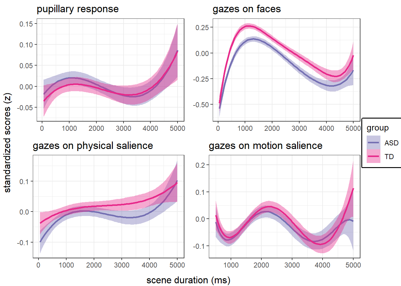
main analyses

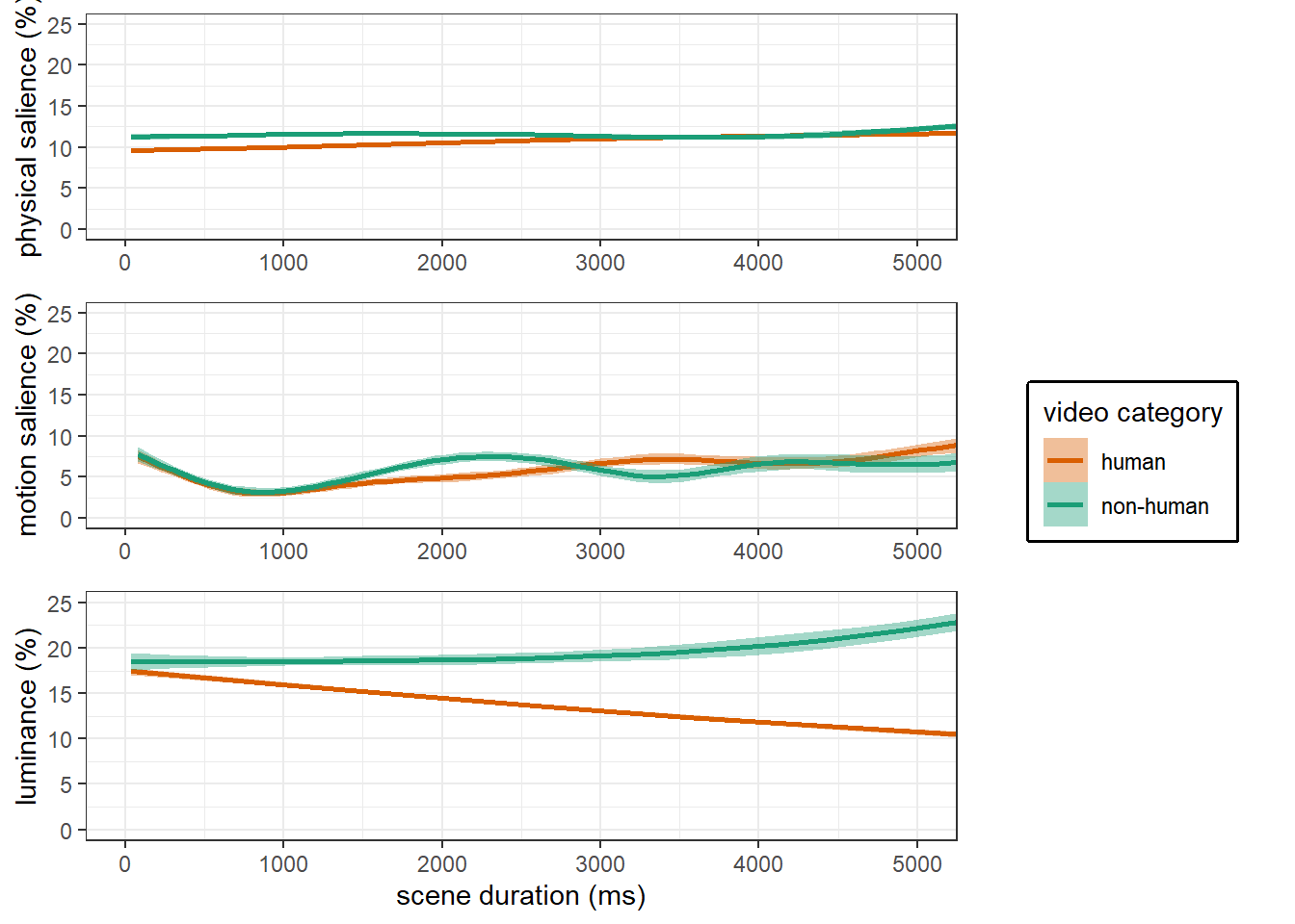
sensory salience

                     2.5 % 97.5 %
vid_socialTRUE -0.32 -0.46  -0.18

            2.5 % 97.5 %
rpd_z -0.03 -0.05  -0.01

 contrast     estimate     SE  df asymp.LCL asymp.UCL
 FALSE - TRUE    0.303 0.0706 Inf     0.164     0.441

Results are averaged over the levels of: t1_diagnosis, t1_sex 
Note: contrasts are still on the scale scale 
Degrees-of-freedom method: asymptotic 
Confidence level used: 0.95 

 vid_social rpd_z.trend      SE  df asymp.LCL asymp.UCL
 FALSE          -0.0368 0.00818 Inf   -0.0529  -0.02081
  TRUE          -0.0115 0.00929 Inf   -0.0298   0.00667

Results are averaged over the levels of: t1_diagnosis, t1_sex 
Degrees-of-freedom method: asymptotic 
Confidence level used: 0.95 

Linear mixed model: physical salience

	Sum Sq	df1	df2	F	p	p_adj
group	2.452	1	255.985	2.892	0.090	0.270
pupillary response (PR)	19.264	1	50077.514	22.718	0.000	0.000
video category (VC)	16.627	1	74.058	19.609	0.000	0.000
time^1	6.380	1	60383.221	7.524	0.006	0.018
time^2	3.466	1	60402.842	4.088	0.043	0.129
time^3	2.010	1	60409.761	2.370	0.124	0.372
sex	0.034	1	233.071	0.040	0.842	1.000
age	0.633	1	260.651	0.746	0.388	1.000
perceptual IQ	0.858	1	255.764	1.012	0.315	0.945
ADHD inattention	0.729	1	260.368	0.859	0.355	1.000
anxiety	1.503	1	200.375	1.772	0.185	0.555
depression	0.572	1	214.709	0.674	0.412	1.000
accuracy	0.631	1	290.413	0.745	0.389	1.000
precision	0.107	1	355.764	0.127	0.722	1.000
center deviation	601.857	1	55270.456	709.762	0.000	0.000
luminance	6.081	1	5226.350	7.171	0.007	0.021
group x PR	1.422	1	52203.539	1.676	0.195	0.585
group x VC	0.863	1	45266.169	1.017	0.313	0.939
PR x VC	7.781	1	23092.014	9.177	0.002	0.006
group x time^1	0.045	1	60332.853	0.053	0.818	1.000
group x time^2	0.020	1	60344.828	0.024	0.878	1.000
group x time^3	0.012	1	60347.178	0.015	0.904	1.000
PR x time^1	0.089	1	60361.277	0.104	0.747	1.000
PR x time^2	0.001	1	60384.879	0.001	0.979	1.000
PR x time^3	0.018	1	60391.595	0.021	0.883	1.000
VC x time^1	0.705	1	60396.575	0.831	0.362	1.000
VC x time^2	2.031	1	60412.980	2.395	0.122	0.366
VC x time^3	2.045	1	60422.044	2.412	0.120	0.360
group x PR x VC	0.025	1	25032.049	0.030	0.863	1.000
group x PR x time^1	0.801	1	60355.653	0.944	0.331	0.993
group x PR x time^2	0.335	1	60378.604	0.395	0.530	1.000
group x PR x time^3	0.100	1	60383.294	0.118	0.731	1.000
group x VC x time^1	0.061	1	60349.925	0.072	0.789	1.000
group x VC x time^2	0.026	1	60363.250	0.031	0.860	1.000
group x VC x time^3	0.013	1	60362.491	0.016	0.900	1.000
PR x VC x time^1	0.758	1	60368.465	0.893	0.345	1.000
PR x VC x time^2	0.625	1	60384.248	0.737	0.391	1.000
PR x VC x time^3	0.881	1	60385.331	1.039	0.308	0.924
group x PR x VC x time^1	1.980	1	60352.732	2.335	0.127	0.381
group x PR x VC x time^2	2.143	1	60369.720	2.527	0.112	0.336
group x PR x VC x time^3	2.078	1	60372.326	2.450	0.117	0.351

Linear mixed model: motion salience

	Sum Sq	df1	df2	F	p	p_adj
group	0.011	1	266.263	0.013	0.910	1.000
pupillary response (PR)	0.521	1	37749.348	0.576	0.448	1.000
video category (VC)	3.307	1	77.178	3.659	0.059	0.177
time^1	162.528	1	60460.016	179.856	0.000	0.000
time^2	156.434	1	60472.791	173.112	0.000	0.000
time^3	135.227	1	60477.847	149.644	0.000	0.000
sex	0.007	1	224.167	0.008	0.928	1.000
age	0.277	1	257.570	0.307	0.580	1.000
perceptual IQ	0.153	1	237.975	0.169	0.681	1.000
ADHD inattention	0.534	1	268.147	0.591	0.443	1.000
anxiety	0.021	1	183.443	0.023	0.878	1.000
depression	0.049	1	208.174	0.054	0.817	1.000
accuracy	0.789	1	347.071	0.873	0.351	1.000
precision	1.227	1	457.477	1.358	0.245	0.735
center deviation	72.929	1	45083.562	80.704	0.000	0.000
luminance	2.870	1	8189.613	3.176	0.075	0.225
group x PR	1.570	1	40994.681	1.738	0.187	0.561
group x VC	0.465	1	38807.474	0.514	0.473	1.000
PR x VC	0.116	1	10454.605	0.128	0.721	1.000
group x time^1	1.110	1	60420.469	1.228	0.268	0.804
group x time^2	0.505	1	60426.347	0.559	0.455	1.000
group x time^3	0.267	1	60426.832	0.296	0.587	1.000
PR x time^1	0.490	1	60435.585	0.542	0.462	1.000
PR x time^2	1.334	1	60443.048	1.476	0.224	0.672
PR x time^3	1.879	1	60443.185	2.079	0.149	0.447
VC x time^1	3.570	1	60466.539	3.950	0.047	0.141
VC x time^2	5.010	1	60475.764	5.544	0.019	0.057
VC x time^3	7.066	1	60481.539	7.820	0.005	0.015
group x PR x VC	0.046	1	12426.176	0.051	0.821	1.000
group x PR x time^1	0.058	1	60430.323	0.064	0.800	1.000
group x PR x time^2	0.012	1	60433.107	0.013	0.908	1.000
group x PR x time^3	0.119	1	60432.031	0.131	0.717	1.000
group x VC x time^1	0.195	1	60426.810	0.215	0.643	1.000
group x VC x time^2	0.401	1	60431.023	0.444	0.505	1.000
group x VC x time^3	0.657	1	60430.932	0.727	0.394	1.000
PR x VC x time^1	21.441	1	60439.836	23.726	0.000	0.000
PR x VC x time^2	28.245	1	60443.100	31.256	0.000	0.000
PR x VC x time^3	30.210	1	60442.944	33.431	0.000	0.000
group x PR x VC x time^1	0.116	1	60430.735	0.128	0.720	1.000
group x PR x VC x time^2	0.002	1	60433.282	0.003	0.958	1.000
group x PR x VC x time^3	0.026	1	60432.961	0.029	0.865	1.000

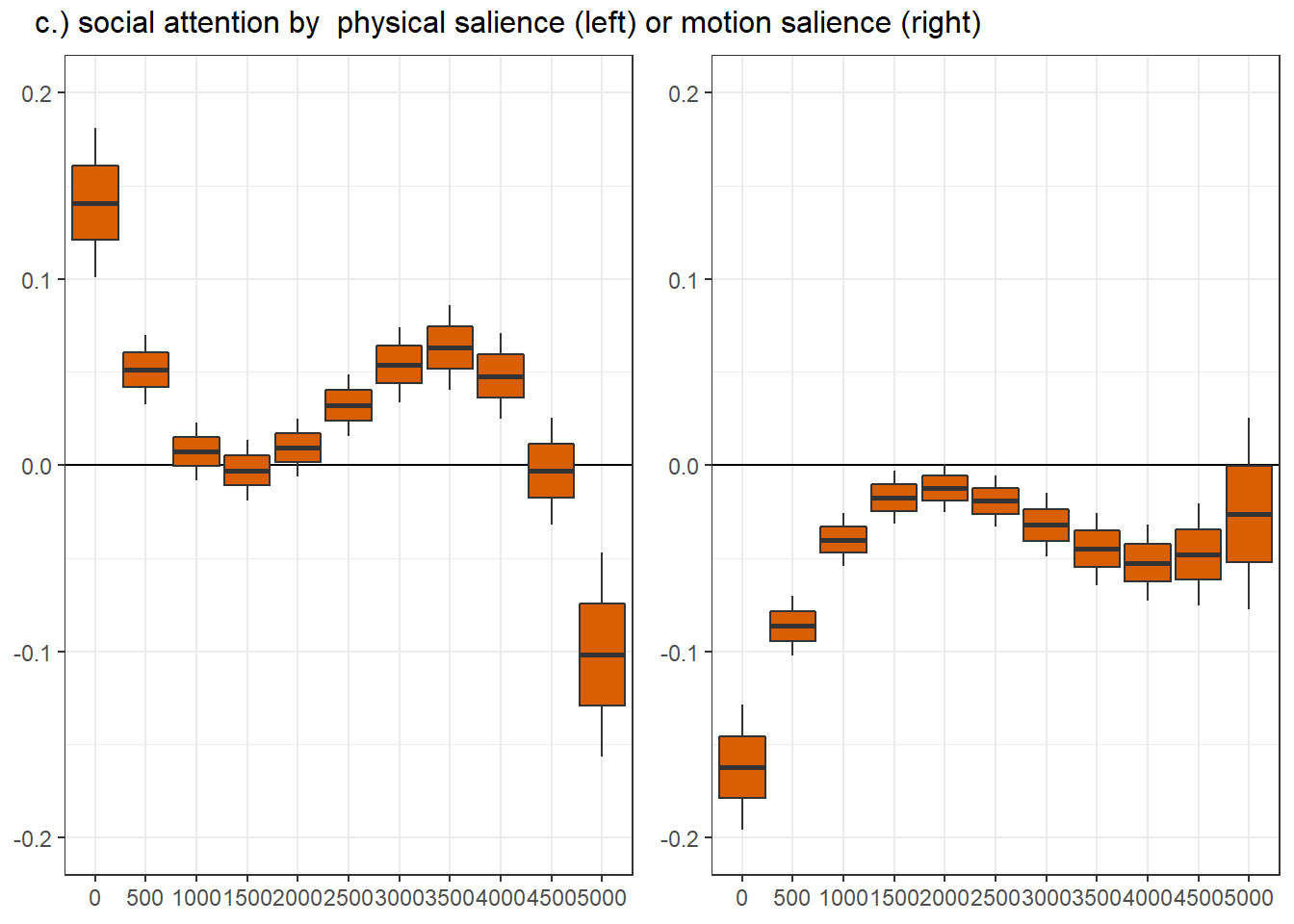
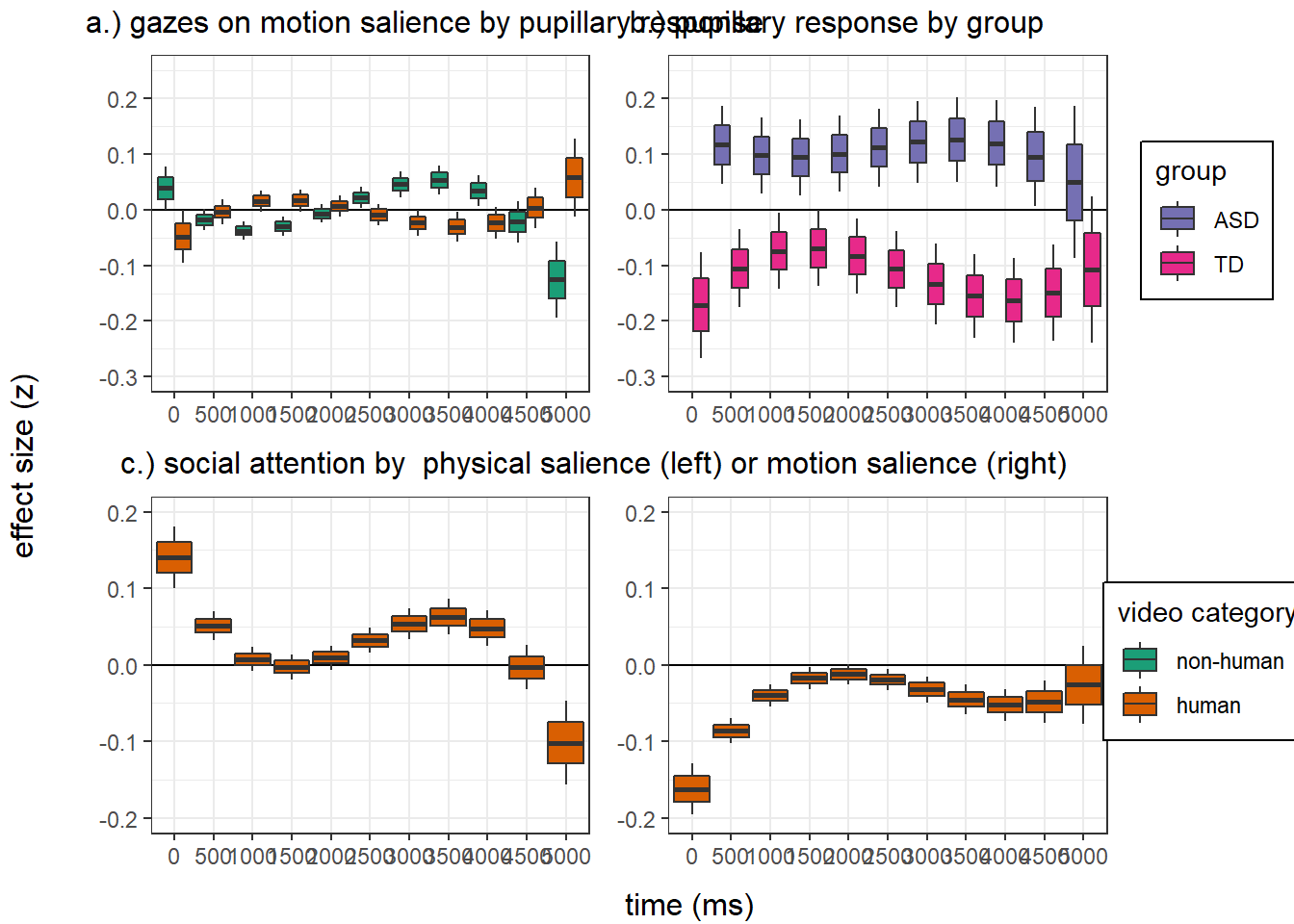
 vid_social ts.scene rpd_z.trend      SE  df asymp.LCL asymp.UCL
 FALSE          1000     -0.0376 0.00849 Inf  -0.05427 -0.020979
  TRUE          1000      0.0154 0.00962 Inf  -0.00342  0.034283
 FALSE          3000      0.0455 0.01160 Inf   0.02281  0.068263
  TRUE          3000     -0.0237 0.01189 Inf  -0.04700 -0.000379

Results are averaged over the levels of: t1_diagnosis, t1_sex 
Degrees-of-freedom method: asymptotic 
Confidence level used: 0.95 

pupillary response

Linear mixed model: pupillary response

	Sum Sq	df1	df2	F	p	p_adj
group	0.002	1	301.764	0.003	0.954	1.000
video category (VC)	15.431	1	78.138	21.252	0.000	0.000
time^1	1.281	1	60190.477	1.765	0.184	0.552
time^2	1.222	1	60195.699	1.683	0.195	0.585
time^3	0.913	1	60198.634	1.257	0.262	0.786
sex	0.416	1	303.843	0.573	0.449	1.000
age	0.250	1	314.546	0.344	0.558	1.000
perceptual IQ	1.132	1	313.407	1.559	0.213	0.639
ADHD inattention	0.160	1	309.328	0.220	0.639	1.000
anxiety	2.931	1	294.514	4.037	0.045	0.135
depression	0.978	1	297.002	1.347	0.247	0.741
accuracy	0.000	1	312.085	0.000	0.984	1.000
precision	0.003	1	331.139	0.004	0.951	1.000
center deviation	333.439	1	60448.581	459.205	0.000	0.000
luminance	0.017	1	25590.455	0.023	0.880	1.000
group x VC	159.276	1	60337.877	219.352	0.000	0.000
group x time^1	0.365	1	60169.957	0.503	0.478	1.000
group x time^2	0.335	1	60173.710	0.461	0.497	1.000
group x time^3	0.194	1	60174.954	0.268	0.605	1.000
VC x time^1	1.192	1	60200.641	1.642	0.200	0.600
VC x time^2	1.149	1	60204.672	1.582	0.208	0.624
VC x time^3	1.641	1	60208.101	2.261	0.133	0.399
group x VC x time^1	5.974	1	60180.107	8.228	0.004	0.012
group x VC x time^2	5.904	1	60184.079	8.130	0.004	0.012
group x VC x time^3	5.101	1	60183.608	7.025	0.008	0.024

                   2.5 % 97.5 %
vid_socialTRUE 0.4  0.19   0.62

vid_social = FALSE:
 contrast      estimate     SE  df asymp.LCL asymp.UCL
 ASD - Control   0.0978 0.0342 Inf    0.0308     0.165

vid_social =  TRUE:
 contrast      estimate     SE  df asymp.LCL asymp.UCL
 ASD - Control  -0.0775 0.0339 Inf   -0.1439    -0.011

Results are averaged over the levels of: t1_sex 
Degrees-of-freedom method: asymptotic 
Confidence level used: 0.95 

vid_social = FALSE, ts.scene =    0:
 contrast      estimate     SE  df asymp.LCL asymp.UCL
 ASD - Control   0.1560 0.0475 Inf    0.0628    0.2491

vid_social =  TRUE, ts.scene =    0:
 contrast      estimate     SE  df asymp.LCL asymp.UCL
 ASD - Control  -0.1716 0.0476 Inf   -0.2649   -0.0783

vid_social = FALSE, ts.scene = 1000:
 contrast      estimate     SE  df asymp.LCL asymp.UCL
 ASD - Control   0.0975 0.0342 Inf    0.0305    0.1646

vid_social =  TRUE, ts.scene = 1000:
 contrast      estimate     SE  df asymp.LCL asymp.UCL
 ASD - Control  -0.0744 0.0340 Inf   -0.1410   -0.0077

vid_social = FALSE, ts.scene = 2000:
 contrast      estimate     SE  df asymp.LCL asymp.UCL
 ASD - Control   0.1004 0.0341 Inf    0.0335    0.1673

vid_social =  TRUE, ts.scene = 2000:
 contrast      estimate     SE  df asymp.LCL asymp.UCL
 ASD - Control  -0.0828 0.0338 Inf   -0.1490   -0.0165

vid_social = FALSE, ts.scene = 3000:
 contrast      estimate     SE  df asymp.LCL asymp.UCL
 ASD - Control   0.1218 0.0368 Inf    0.0498    0.1939

vid_social =  TRUE, ts.scene = 3000:
 contrast      estimate     SE  df asymp.LCL asymp.UCL
 ASD - Control  -0.1334 0.0360 Inf   -0.2039   -0.0628

vid_social = FALSE, ts.scene = 4000:
 contrast      estimate     SE  df asymp.LCL asymp.UCL
 ASD - Control   0.1192 0.0389 Inf    0.0430    0.1953

vid_social =  TRUE, ts.scene = 4000:
 contrast      estimate     SE  df asymp.LCL asymp.UCL
 ASD - Control  -0.1627 0.0381 Inf   -0.2374   -0.0880

vid_social = FALSE, ts.scene = 5000:
 contrast      estimate     SE  df asymp.LCL asymp.UCL
 ASD - Control   0.0497 0.0682 Inf   -0.0841    0.1834

vid_social =  TRUE, ts.scene = 5000:
 contrast      estimate     SE  df asymp.LCL asymp.UCL
 ASD - Control  -0.1074 0.0656 Inf   -0.2359    0.0211

Results are averaged over the levels of: t1_sex 
Degrees-of-freedom method: asymptotic 
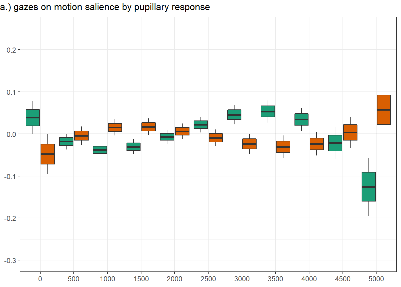
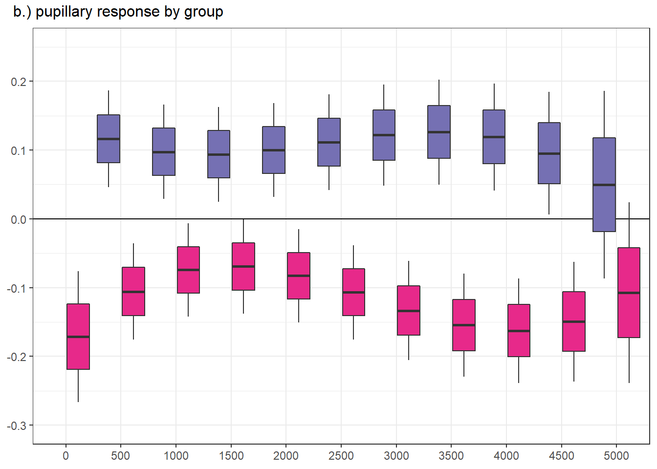
Confidence level used: 0.95 

gaze on face (social attention)

Linear mixed model: social attention without mediators

	Sum Sq	df1	df2	F	p	p_adj
group	3.355	1	290.297	5.965	0.015	0.045
time^1	491.695	1	30849.946	874.130	0.000	0.000
time^2	393.258	1	30856.811	699.129	0.000	0.000
time^3	340.445	1	30853.309	605.238	0.000	0.000
sex	2.057	1	288.885	3.657	0.057	0.171
age	13.905	1	294.278	24.720	0.000	0.000
perceptual IQ	6.416	1	297.524	11.407	0.001	0.003
ADHD inattention	1.087	1	293.475	1.933	0.166	0.498
anxiety	1.095	1	276.850	1.946	0.164	0.492
depression	1.898	1	282.560	3.375	0.067	0.201
accuracy	1.776	1	297.211	3.158	0.077	0.231
precision	1.008	1	322.502	1.793	0.182	0.546
center deviation	0.004	1	31068.238	0.007	0.933	1.000
luminance	23.697	1	479.647	42.128	0.000	0.000
group x time^1	0.013	1	30819.318	0.022	0.881	1.000
group x time^2	0.003	1	30825.065	0.005	0.944	1.000
group x time^3	0.003	1	30824.931	0.005	0.942	1.000

                         2.5 % 97.5 %
t1_diagnosisControl 0.08  0.02   0.15

Linear mixed model: social attention with motion salience and physical salience as mediators

	Sum Sq	df1	df2	F	p	p_adj
group	3.155	1	292.178	5.643	0.018	0.054
motion salience (MS)	51.119	1	30857.849	91.425	0.000	0.000
physical salience (PS)	15.817	1	30872.066	28.287	0.000	0.000
time^1	398.929	1	30836.718	713.472	0.000	0.000
time^2	318.188	1	30846.006	569.070	0.000	0.000
time^3	275.996	1	30840.279	493.612	0.000	0.000
sex	2.086	1	289.494	3.730	0.054	0.162
age	14.187	1	294.882	25.373	0.000	0.000
perceptual IQ	6.431	1	298.168	11.503	0.001	0.003
ADHD inattention	1.103	1	294.085	1.972	0.161	0.483
anxiety	1.122	1	277.475	2.006	0.158	0.474
depression	1.924	1	283.165	3.441	0.065	0.195
accuracy	1.780	1	297.813	3.183	0.075	0.225
precision	0.982	1	323.141	1.757	0.186	0.558
center deviation	0.051	1	31045.911	0.091	0.763	1.000
luminance	16.686	1	492.182	29.842	0.000	0.000
group x MS	1.090	1	30831.156	1.950	0.163	0.489
group x PS	0.001	1	30872.661	0.002	0.966	1.000
group x time^1	0.000	1	30809.259	0.000	0.997	1.000
group x time^2	0.001	1	30814.174	0.002	0.968	1.000
group x time^3	0.000	1	30813.100	0.000	0.992	1.000
MS x time^1	19.861	1	30859.132	35.521	0.000	0.000
MS x time^2	11.697	1	30845.642	20.920	0.000	0.000
MS x time^3	7.508	1	30835.811	13.427	0.000	0.000
PS x time^1	22.938	1	30827.690	41.024	0.000	0.000
PS x time^2	23.161	1	30825.468	41.423	0.000	0.000
PS x time^3	22.736	1	30824.048	40.663	0.000	0.000
group x MS x time^1	0.051	1	30848.104	0.091	0.764	1.000
group x MS x time^2	0.001	1	30851.315	0.001	0.974	1.000
group x MS x time^3	0.049	1	30849.607	0.087	0.768	1.000
group x PS x time^1	0.009	1	30820.235	0.017	0.897	1.000
group x PS x time^2	0.003	1	30814.283	0.005	0.942	1.000
group x PS x time^3	0.002	1	30810.674	0.003	0.957	1.000

                       2.5 % 97.5 %
lowlvl_salience_z 0.03  0.01   0.04

                        2.5 % 97.5 %
motion_salience_z -0.04 -0.05  -0.03

Linear mixed model: social attention with pupillary response as mediator

	Sum Sq	df1	df2	F	p	p_adj
group	2.617	1	297.170	4.655	0.032	0.096
pupillary response (PR)	2.466	1	29778.861	4.387	0.036	0.108
time^1	481.333	1	30842.220	856.300	0.000	0.000
time^2	383.359	1	30853.202	682.002	0.000	0.000
time^3	330.236	1	30850.828	587.496	0.000	0.000
sex	2.033	1	289.459	3.616	0.058	0.174
age	13.783	1	294.891	24.520	0.000	0.000
perceptual IQ	6.627	1	298.210	11.790	0.001	0.003
ADHD inattention	1.139	1	293.986	2.026	0.156	0.468
anxiety	1.050	1	277.372	1.868	0.173	0.519
depression	1.816	1	283.029	3.231	0.073	0.219
accuracy	1.776	1	297.598	3.159	0.077	0.231
precision	1.036	1	322.910	1.844	0.175	0.525
center deviation	0.000	1	31062.568	0.000	0.987	1.000
luminance	23.577	1	478.199	41.944	0.000	0.000
group x PR	4.100	1	30110.046	7.295	0.007	0.021
group x time^1	0.080	1	30815.200	0.143	0.706	1.000
group x time^2	0.089	1	30823.130	0.158	0.691	1.000
group x time^3	0.083	1	30825.588	0.148	0.700	1.000
PR x time^1	7.203	1	30823.078	12.814	0.000	0.000
PR x time^2	6.051	1	30829.089	10.765	0.001	0.003
PR x time^3	5.220	1	30831.156	9.286	0.002	0.006
group x PR x time^1	0.319	1	30820.563	0.568	0.451	1.000
group x PR x time^2	0.216	1	30826.132	0.384	0.536	1.000
group x PR x time^3	0.213	1	30828.816	0.378	0.539	1.000

 t1_diagnosis rpd_z.trend     SE  df asymp.LCL asymp.UCL
 ASD              -0.0402 0.0120 Inf   -0.0637  -0.01659
 Control          -0.0148 0.0099 Inf   -0.0342   0.00461

Results are averaged over the levels of: t1_sex 
Degrees-of-freedom method: asymptotic 
Confidence level used: 0.95 

Linear mixed model: social attention with pupillary components as mediator

	Sum Sq	df1	df2	F	p	p_adj
group	2.825	1	296.418	4.870	0.028	0.084
early pupillary comp. (PC1)	30.062	1	30758.287	51.822	0.000	0.000
late pupillary comp. (PC2)	15.182	1	31025.249	26.172	0.000	0.000
sex	2.150	1	288.637	3.706	0.055	0.165
age	13.873	1	294.233	23.914	0.000	0.000
perceptual IQ	6.748	1	297.520	11.633	0.001	0.003
ADHD inattention	1.309	1	293.304	2.256	0.134	0.402
anxiety	0.995	1	276.315	1.716	0.191	0.573
depression	1.895	1	282.113	3.268	0.072	0.216
accuracy	1.781	1	297.005	3.070	0.081	0.243
precision	1.109	1	322.660	1.913	0.168	0.504
center deviation	0.020	1	31076.345	0.035	0.851	1.000
luminance	28.982	1	457.457	49.961	0.000	0.000
group x PC1	1.152	1	30976.345	1.986	0.159	0.477
group x PC2	1.894	1	30996.355	3.265	0.071	0.213

                2.5 % 97.5 %
rpd_RC1_z -0.04 -0.06  -0.03

               2.5 % 97.5 %
rpd_RC2_z 0.02     0   0.03

panel figure - temporal effects

png 
  2 

Session information

R version 3.6.1 (2019-07-05)
Platform: x86_64-w64-mingw32/x64 (64-bit)
Running under: Windows 10 x64 (build 19043)

Matrix products: default

locale:
[1] LC_COLLATE=German_Germany.1252  LC_CTYPE=German_Germany.1252   
[3] LC_MONETARY=German_Germany.1252 LC_NUMERIC=C                   
[5] LC_TIME=German_Germany.1252    

attached base packages:
[1] stats     graphics  grDevices utils     datasets  methods   base     

other attached packages:
 [1] simr_1.0.5       missMDA_1.18     psych_1.9.12.31  MuMIn_1.43.17   
 [5] emmeans_1.4.3.01 lmerTest_3.1-2   lme4_1.1-23      Matrix_1.2-18   
 [9] kableExtra_1.3.1 gridExtra_2.3    sjmisc_2.8.5     sjPlot_2.8.5    
[13] ggplot2_3.2.1    reshape2_1.4.3   R.matlab_3.6.2   MatchIt_3.0.2   
[17] Gmisc_1.11.0     htmlTable_2.1.0  Rcpp_1.0.3       mice_3.7.0      
[21] lattice_0.20-38  zoo_1.8-6        readxl_1.3.1    

loaded via a namespace (and not attached):
  [1] backports_1.1.5      Hmisc_4.3-0          workflowr_1.6.2     
  [4] plyr_1.8.5           lazyeval_0.2.2       splines_3.6.1       
  [7] RLRsim_3.1-3         digest_0.6.23        foreach_1.5.1       
 [10] htmltools_0.4.0      magrittr_1.5         checkmate_1.9.4     
 [13] cluster_2.1.0        doParallel_1.0.16    openxlsx_4.1.4      
 [16] modelr_0.1.5         R.utils_2.9.2        jpeg_0.1-8.1        
 [19] colorspace_1.4-1     rvest_0.3.5          ggrepel_0.8.1       
 [22] haven_2.2.0          pan_1.6              xfun_0.11           
 [25] dplyr_1.0.2          crayon_1.3.4         survival_3.1-8      
 [28] iterators_1.0.12     glue_1.4.2           gtable_0.3.0        
 [31] webshot_0.5.2        sjstats_0.18.0       car_3.0-6           
 [34] jomo_2.6-10          abind_1.4-5          scales_1.1.0        
 [37] mvtnorm_1.0-11       ggeffects_0.16.0     plotrix_3.7-7       
 [40] viridisLite_0.3.0    xtable_1.8-4         performance_0.5.0   
 [43] flashClust_1.01-2    foreign_0.8-74       Formula_1.2-3       
 [46] stats4_3.6.1         DT_0.11              htmlwidgets_1.5.1   
 [49] httr_1.4.1           RColorBrewer_1.1-2   acepack_1.4.1       
 [52] ellipsis_0.3.0       pkgconfig_2.0.3      XML_3.99-0.3        
 [55] R.methodsS3_1.7.1    binom_1.1-1          nnet_7.3-12         
 [58] tidyselect_1.1.0     rlang_0.4.8          later_1.0.0         
 [61] effectsize_0.0.1     munsell_0.5.0        cellranger_1.1.0    
 [64] tools_3.6.1          generics_0.0.2       sjlabelled_1.1.6    
 [67] broom_0.7.2          evaluate_0.14        stringr_1.4.0       
 [70] yaml_2.2.0           knitr_1.26           fs_1.3.1            
 [73] zip_2.0.4            forestplot_1.10      purrr_0.3.3         
 [76] mitml_0.3-7          nlme_3.1-143         R.oo_1.23.0         
 [79] leaps_3.1            xml2_1.2.2           pbkrtest_0.4-7      
 [82] compiler_3.6.1       rstudioapi_0.10      curl_4.3            
 [85] png_0.1-7            tibble_3.0.4         statmod_1.4.34      
 [88] stringi_1.4.5        highr_0.8            parameters_0.8.5    
 [91] forcats_0.4.0        nloptr_1.2.1         vctrs_0.3.4         
 [94] pillar_1.4.3         lifecycle_0.2.0      estimability_1.3    
 [97] data.table_1.12.8    insight_0.9.6        httpuv_1.5.2        
[100] R6_2.4.1             latticeExtra_0.6-29  promises_1.1.0      
[103] rio_0.5.16           codetools_0.2-16     boot_1.3-24         
[106] MASS_7.3-51.5        rprojroot_1.3-2      withr_2.1.2         
[109] mnormt_1.5-5         hms_0.5.3            mgcv_1.8-31         
[112] bayestestR_0.7.2     parallel_3.6.1       grid_3.6.1          
[115] rpart_4.1-15         tidyr_1.0.0          coda_0.19-4         
[118] minqa_1.2.4          rmarkdown_2.0        carData_3.0-3       
[121] git2r_0.26.1         numDeriv_2016.8-1.1  scatterplot3d_0.3-41
[124] lubridate_1.7.9      base64enc_0.1-3      FactoMineR_2.4