Multiple Comparison and Mean Expression
Last updated: 2022-11-29
Checks: 7 0
Knit directory: dgrp-starve/
This reproducible R Markdown analysis was created with workflowr (version 1.7.0). The Checks tab describes the reproducibility checks that were applied when the results were created. The Past versions tab lists the development history.
Great! Since the R Markdown file has been committed to the Git repository, you know the exact version of the code that produced these results.
Great job! The global environment was empty. Objects defined in the global environment can affect the analysis in your R Markdown file in unknown ways. For reproduciblity it’s best to always run the code in an empty environment.
The command set.seed(20221101) was run prior to running
the code in the R Markdown file. Setting a seed ensures that any results
that rely on randomness, e.g. subsampling or permutations, are
reproducible.
Great job! Recording the operating system, R version, and package versions is critical for reproducibility.
Nice! There were no cached chunks for this analysis, so you can be confident that you successfully produced the results during this run.
Great job! Using relative paths to the files within your workflowr project makes it easier to run your code on other machines.
Great! You are using Git for version control. Tracking code development and connecting the code version to the results is critical for reproducibility.
The results in this page were generated with repository version 6cb699d. See the Past versions tab to see a history of the changes made to the R Markdown and HTML files.
Note that you need to be careful to ensure that all relevant files for
the analysis have been committed to Git prior to generating the results
(you can use wflow_publish or
wflow_git_commit). workflowr only checks the R Markdown
file, but you know if there are other scripts or data files that it
depends on. Below is the status of the Git repository when the results
were generated:
Untracked files:
    Untracked:  code/analysisSR.R
    Untracked:  code/geneGO.R
    Untracked:  code/multiPrep.R
    Untracked:  code/snpGene.77509.err
    Untracked:  code/snpGene.77509.out
    Untracked:  code/snpGene.77515.err
    Untracked:  code/snpGene.77515.out
    Untracked:  code/snpGene.sbatch
    Untracked:  data/eQTL_traits_females.csv
    Untracked:  data/eQTL_traits_males.csv
    Untracked:  data/goGroups.txt
    Untracked:  data/xp-f.txt
    Untracked:  data/xp-m.txt
    Untracked:  scoreAnalysisMulticomp.R
    Untracked:  temp.Rmd

Unstaged changes:
    Deleted:    analysis/database.Rmd
    Modified:   code/baseScript-lineComp.R
    Modified:   code/fourLinePrep.R
Note that any generated files, e.g. HTML, png, CSS, etc., are not included in this status report because it is ok for generated content to have uncommitted changes.
These are the previous versions of the repository in which changes were
made to the R Markdown (analysis/multiComp.Rmd) and HTML
(docs/multiComp.html) files. If you’ve configured a remote
Git repository (see ?wflow_git_remote), click on the
hyperlinks in the table below to view the files as they were in that
past version.
| File | Version | Author | Date | Message |
|---|---|---|---|---|
| Rmd | 6cb699d | nklimko | 2022-11-29 | wflow_publish("analysis/*") |
| html | 37f3436 | nklimko | 2022-11-22 | Build site. |
| Rmd | 638d414 | nklimko | 2022-11-22 | wflow_publish("analysis/multiComp.Rmd") |
| html | c8859ee | nklimko | 2022-11-22 | Build site. |
| Rmd | 68bd7e9 | nklimko | 2022-11-22 | wflow_publish("analysis/multiComp.Rmd") |
| html | 37278c9 | nklimko | 2022-11-22 | Build site. |
| Rmd | e82e73c | nklimko | 2022-11-22 | wflow_publish("analysis/*") |
| html | f09779e | nklimko | 2022-11-22 | Build site. |
| Rmd | fc90dac | nklimko | 2022-11-22 | wflow_publish("analysis/*") |
| html | f1d6437 | nklimko | 2022-11-15 | Build site. |
| Rmd | afd22f8 | nklimko | 2022-11-15 | wflow_publish("analysis/*") |
| html | 79e98ca | nklimko | 2022-11-15 | Build site. |
| Rmd | ca79c22 | nklimko | 2022-11-15 | wflow_publish("analysis/*") |
Multiple Comparison
Starvation was plotted against every other trait and correlations were calculated. Ideally, strong correlation between traits can be used to increase the impact of PCA as traits with strong correlations can be used to reduce dimensions. Strong correlations allow for calculated columns.
Female Traits
# Read in tables
dtf <- fread("data/eQTL_traits_females.csv")

#Change column order to line, starvation, everything else
setcolorder(dtf, c(1,10,2:9,11:19))

#Storage structures
corKeep <- rep(0,18)
gg <- vector(mode='list', length=18)

# x axis, starvation
x <- dtf[,2,with=FALSE]

# x Label
xL <- "starvation"

# Determine average of each trait
for(i in 3:19)
{
  #grab column of interest
  y <- dtf[,i,with=FALSE]

  #grab trait name from column name
  yL <- colnames(dtf[, i, with=FALSE])

  #extract non NULL paired data, set to data table, rename columns
  raw <- na.omit(cbind(x,y))
  clean <- setDT(raw)
  colnames(clean) <- c("starvation", "trait")

  #grab correlation coefficient using cor.test
  corCoeff <- str_sub(as.character(cor.test(clean$starvation, clean$trait)[4]), 8,16)
  corKeep[i-1] <- as.numeric(corCoeff)

  #create graph title using y label and include correlation coefficient
  graphTitle <- paste0(yL,": R=",corCoeff)

  #gg plot commands: starvation vs trait, plot dots, trend line, and labels
  gg[[i-1]] <- ggplot(clean, aes(x=starvation, y=trait)) +
  geom_point(color="red") +
  geom_smooth(formula = y ~ x, method=lm) +
  labs(title = graphTitle, x=xL, y=yL)
}

#reorder plots by absolute value of correlation coefficient
gg <- cbind(gg,corKeep)
gg <- gg[order(abs(corKeep),decreasing=TRUE),]
Warning in grid.Call.graphics(C_polygon, x$x, x$y, index): semi-transparency is
not supported on this device: reported only once per page
Warning in grid.Call.graphics(C_polygon, x$x, x$y, index): semi-transparency is
not supported on this device: reported only once per page
Warning in grid.Call.graphics(C_polygon, x$x, x$y, index): semi-transparency is
not supported on this device: reported only once per page
Warning in grid.Call.graphics(C_polygon, x$x, x$y, index): semi-transparency is
not supported on this device: reported only once per page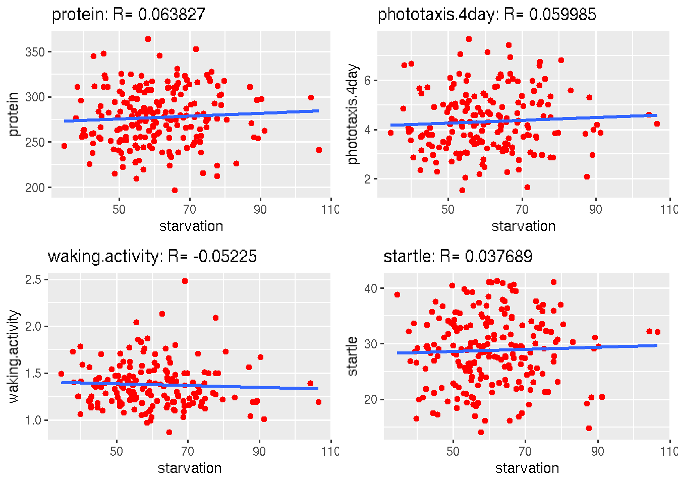
Warning in grid.Call.graphics(C_polygon, x$x, x$y, index): semi-transparency is
not supported on this device: reported only once per page
Male Traits
# Read in tables
dtm <- fread("data/eQTL_traits_males.csv")
#Change column order to line, starvation, everything else
setcolorder(dtm, c(1,11,3:10,12:20,2))
#Storage structures
corKeep <- rep(0,18)
gg <- vector(mode='list', length=18)
# x axis, starvation
x <- dtm[,2,with=FALSE]
# x Label
xL <- "starvation"
# Determine average of each trait
for(i in 3:20)
{
#grab column of interest
y <- dtm[,i,with=FALSE]
#grab trait name from column name
yL <- colnames(dtm[, i, with=FALSE])
#extract non NULL paired data, set to data table, rename columns
raw <- na.omit(cbind(x,y))
clean <- setDT(raw)
colnames(clean) <- c("starvation", "trait")
#grab correlation coefficient using cor.test
corCoeff <- str_sub(as.character(cor.test(clean$starvation, clean$trait)[4]), 8,16)
corKeep[i-1] <- as.numeric(corCoeff)
#create graph title using y label and include correlation coefficient
graphTitle <- paste0(yL,": R=",corCoeff)
#gg plot commands: starvation vs trait, plot dots, trend line, and labels
gg[[i-1]] <- ggplot(clean, aes(x=starvation, y=trait)) +
geom_point() +
geom_smooth(formula = y ~ x, method=lm) +
labs(title = graphTitle, x=xL, y=yL)
}
#reorder plots by absolute value of correlation coefficient
gg <- cbind(gg,corKeep)
gg <- gg[order(abs(corKeep),decreasing=TRUE),]Warning in grid.Call.graphics(C_polygon, x$x, x$y, index): semi-transparency is
not supported on this device: reported only once per page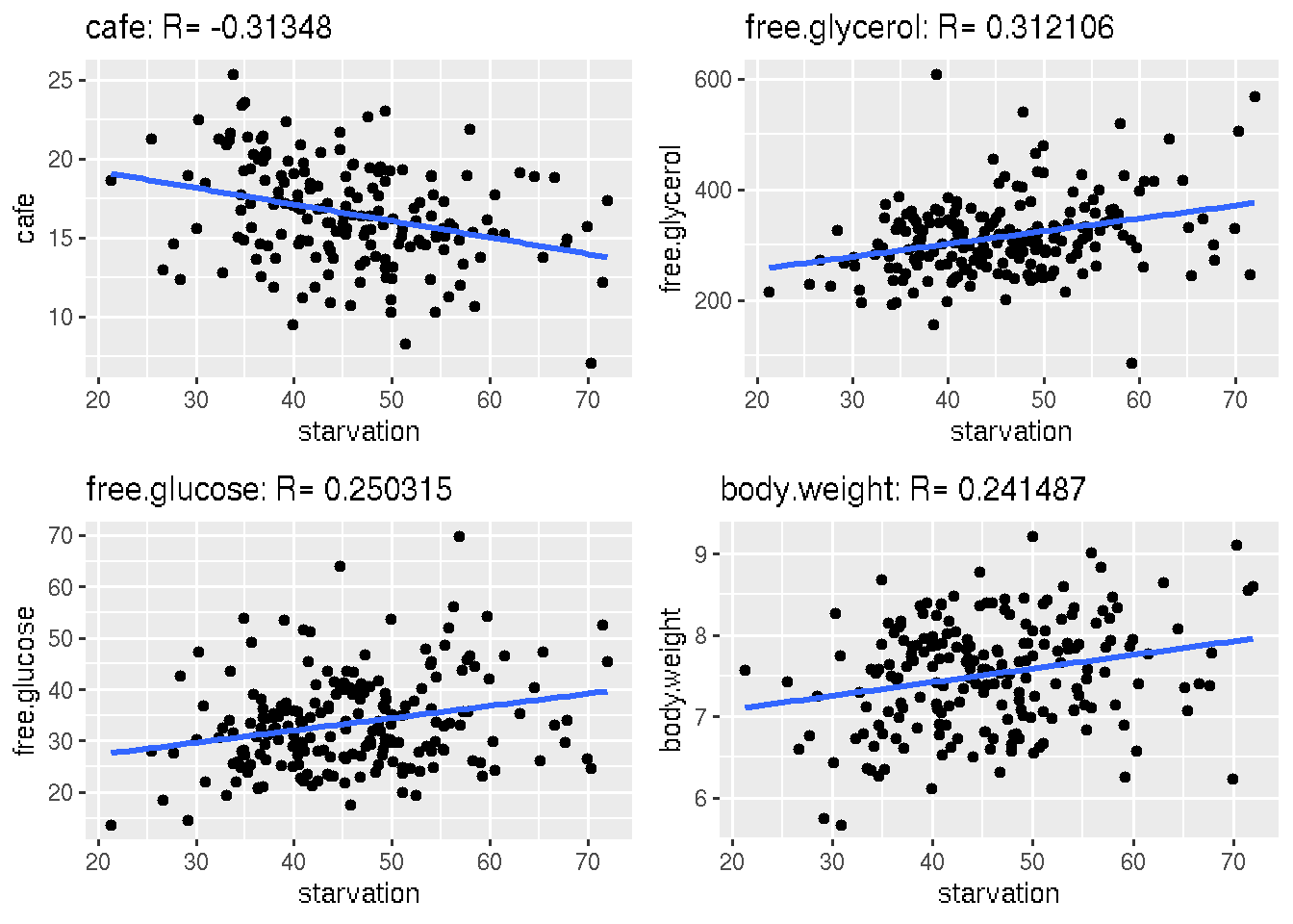
Warning in grid.Call.graphics(C_polygon, x$x, x$y, index): semi-transparency is
not supported on this device: reported only once per page
Warning in grid.Call.graphics(C_polygon, x$x, x$y, index): semi-transparency is
not supported on this device: reported only once per page
Warning in grid.Call.graphics(C_polygon, x$x, x$y, index): semi-transparency is
not supported on this device: reported only once per page
Warning in grid.Call.graphics(C_polygon, x$x, x$y, index): semi-transparency is
not supported on this device: reported only once per page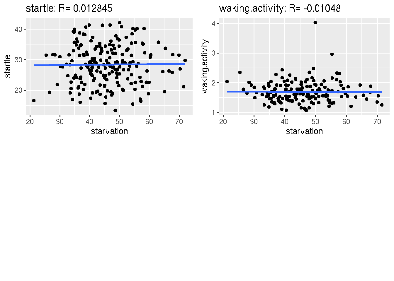
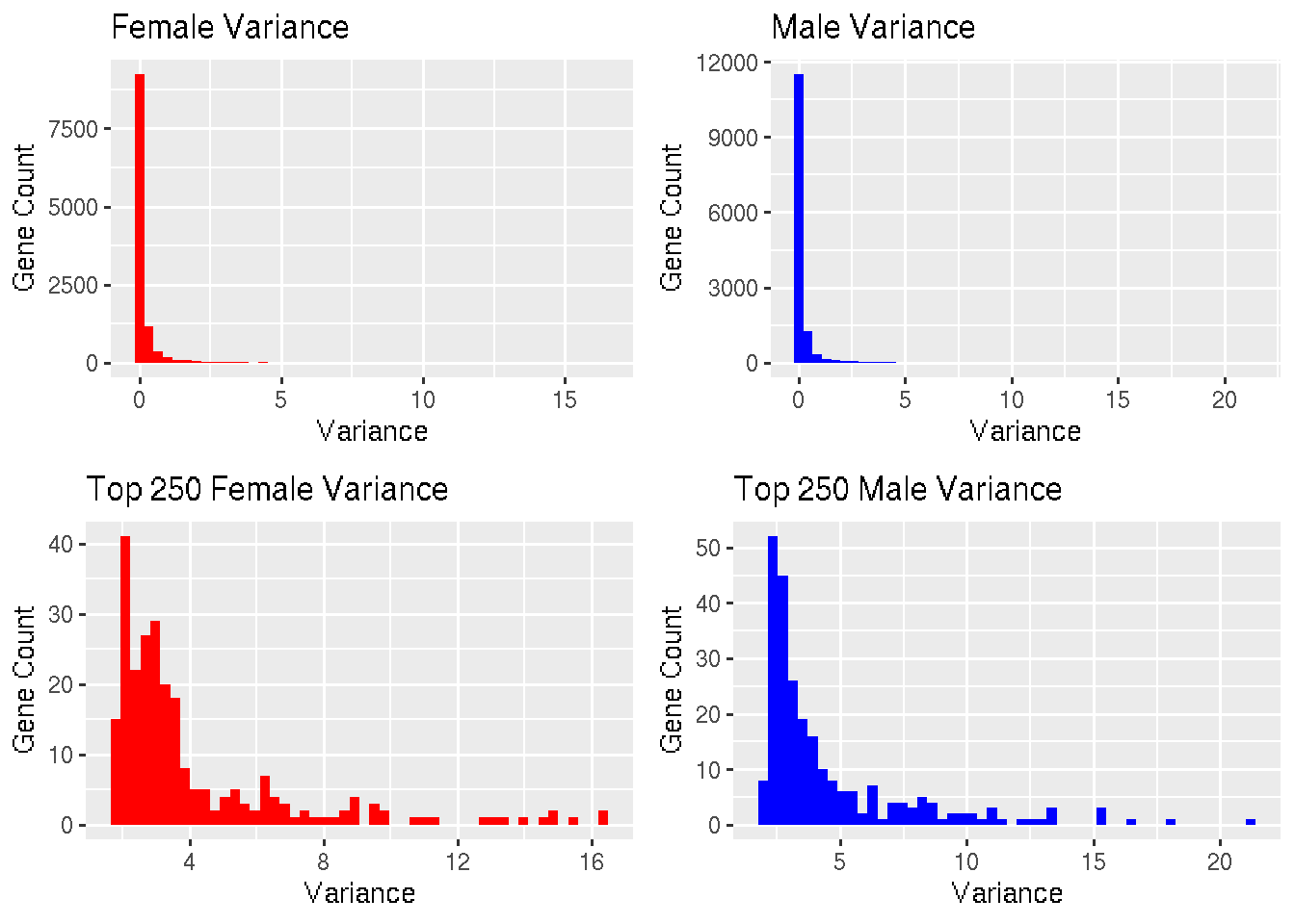
Mean Expression
#read in data
xpf <- fread("data/xp-f.txt")

#remove line, non numeric
xpf <- xpf[,-1]

#colMeans for means of all columns
xpfMean <- colMeans(xpf, na.rm=TRUE)

#sapply to calculate variance of every column
xpfVar <- sapply(xpf, var)

#store final info
xpfStats <- data.table(xpfMean, xpfVar)

#selection of upper regions of histograms
ffilt <- xpfStats[order(xpfStats$xpfVar, decreasing=TRUE)]

ftrim <- ffilt[1:250]
#read in data
xpm <- fread("data/xp-m.txt")
#remove line, non numeric
xpm <- xpm[,-1]
#colMeans for means of all columns
xpmMean <- colMeans(xpm, na.rm=TRUE)
#sapply to calculate variance of every column
xpmVar <- sapply(xpm, var)
#store final info
xpmStats <- data.table(xpmMean, xpmVar)
#selection of upper regions of histograms
mfilt <- xpmStats[order(xpmStats$xpmVar, decreasing=TRUE)]
mtrim <- mfilt[1:250]
Gene Counts
#list input for venn diagram
A <- list('Female'=colnames(xpf), 'Male'=colnames(xpm))

#Venn diagram of gene counts
ggvenn(A, show_percentage = FALSE)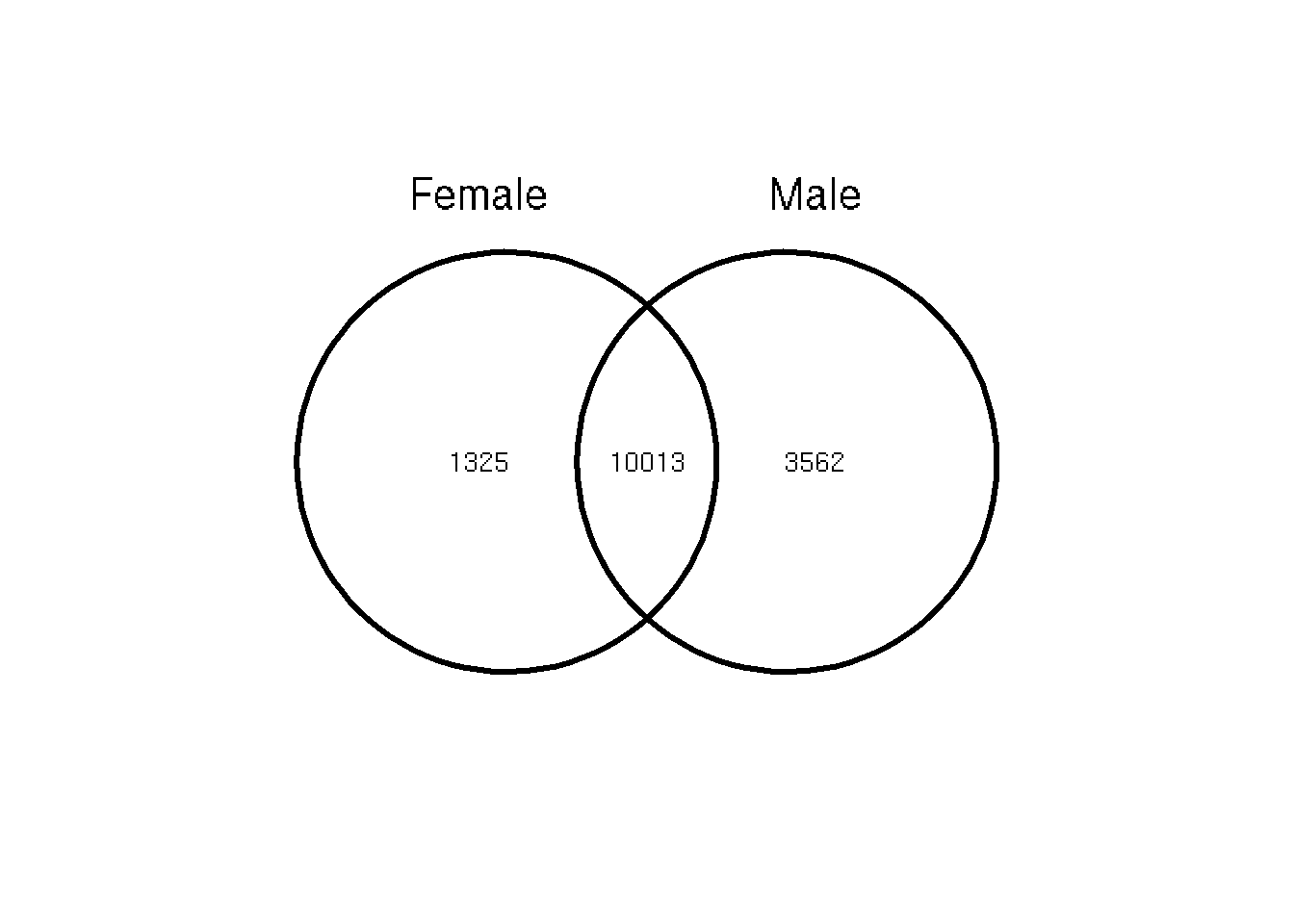
# means converted to data tables for easier join
fMeans <- as.data.table(xpfMean, keep.rownames = TRUE)
mMeans <- as.data.table(xpmMean, keep.rownames = TRUE)

#joined means, nulls omitted
aMeans <- fMeans[mMeans, on = .(rn), nomatch=NULL]

#correlation of male to female expression
corCoeff <- str_sub(as.character(cor.test(aMeans$xpfMean, aMeans$xpmMean)[4]), 8,16)

#gg plot commands: starvation vs trait, plot dots, trend line, and labels
ggplot(aMeans, aes(x=xpfMean, y=xpmMean)) +
geom_point(color="purple") +
geom_smooth(formula = y ~ x, method=lm) +
labs(x="Female Expression", y="Female Expression", subtitle=paste0("R: ",corCoeff)) +
ggtitle("Male vs Female Mean Expression")
Warning in grid.Call.graphics(C_polygon, x$x, x$y, index): semi-transparency is
not supported on this device: reported only once per page
sessionInfo()R version 4.0.3 (2020-10-10)
Platform: x86_64-pc-linux-gnu (64-bit)
Running under: CentOS Linux 7 (Core)
Matrix products: default
BLAS/LAPACK: /opt/ohpc/pub/Software/openblas_0.3.10/lib/libopenblas_haswellp-r0.3.10.dev.so
locale:
[1] LC_CTYPE=en_US.utf-8 LC_NUMERIC=C
[3] LC_TIME=en_US.utf-8 LC_COLLATE=en_US.utf-8
[5] LC_MONETARY=en_US.utf-8 LC_MESSAGES=en_US.utf-8
[7] LC_PAPER=en_US.utf-8 LC_NAME=C
[9] LC_ADDRESS=C LC_TELEPHONE=C
[11] LC_MEASUREMENT=en_US.utf-8 LC_IDENTIFICATION=C
attached base packages:
[1] grid stats graphics grDevices utils datasets methods
[8] base
other attached packages:
[1] ggvenn_0.1.9 cowplot_1.1.1 ggplot2_3.3.5 data.table_1.14.2
[5] stringr_1.4.0 dplyr_1.0.8 workflowr_1.7.0
loaded via a namespace (and not attached):
[1] tidyselect_1.1.2 xfun_0.30 bslib_0.3.1 purrr_0.3.4
[5] lattice_0.20-45 splines_4.0.3 colorspace_2.0-3 vctrs_0.4.1
[9] generics_0.1.2 htmltools_0.5.2 mgcv_1.8-40 yaml_2.3.5
[13] utf8_1.2.2 rlang_1.0.4 later_1.3.0 pillar_1.7.0
[17] jquerylib_0.1.4 withr_2.5.0 glue_1.6.2 DBI_1.1.2
[21] lifecycle_1.0.1 munsell_0.5.0 gtable_0.3.0 evaluate_0.15
[25] labeling_0.4.2 knitr_1.38 callr_3.7.0 fastmap_1.1.0
[29] httpuv_1.6.5 ps_1.6.0 fansi_1.0.3 highr_0.9
[33] Rcpp_1.0.8.3 promises_1.2.0.1 scales_1.2.0 jsonlite_1.8.0
[37] farver_2.1.0 fs_1.5.2 digest_0.6.29 stringi_1.7.6
[41] processx_3.5.3 getPass_0.2-2 rprojroot_2.0.3 cli_3.3.0
[45] tools_4.0.3 magrittr_2.0.3 sass_0.4.1 tibble_3.1.6
[49] crayon_1.5.1 whisker_0.4 pkgconfig_2.0.3 Matrix_1.4-1
[53] ellipsis_0.3.2 assertthat_0.2.1 rmarkdown_2.16 httr_1.4.2
[57] rstudioapi_0.13 R6_2.5.1 nlme_3.1-157 git2r_0.30.1
[61] compiler_4.0.3