Linking yield with NLR PAV
Philipp Bayer
2020-09-22
Last updated: 2020-11-04
Checks: 7 0
Knit directory: R_gene_analysis/
This reproducible R Markdown analysis was created with workflowr (version 1.6.2.9000). The Checks tab describes the reproducibility checks that were applied when the results were created. The Past versions tab lists the development history.
Great! Since the R Markdown file has been committed to the Git repository, you know the exact version of the code that produced these results.
Great job! The global environment was empty. Objects defined in the global environment can affect the analysis in your R Markdown file in unknown ways. For reproduciblity it’s best to always run the code in an empty environment.
The command set.seed(20200917) was run prior to running the code in the R Markdown file. Setting a seed ensures that any results that rely on randomness, e.g. subsampling or permutations, are reproducible.
Great job! Recording the operating system, R version, and package versions is critical for reproducibility.
Nice! There were no cached chunks for this analysis, so you can be confident that you successfully produced the results during this run.
Great job! Using relative paths to the files within your workflowr project makes it easier to run your code on other machines.
Great! You are using Git for version control. Tracking code development and connecting the code version to the results is critical for reproducibility.
The results in this page were generated with repository version 2d9c3db. See the Past versions tab to see a history of the changes made to the R Markdown and HTML files.
Note that you need to be careful to ensure that all relevant files for the analysis have been committed to Git prior to generating the results (you can use wflow_publish or wflow_git_commit). workflowr only checks the R Markdown file, but you know if there are other scripts or data files that it depends on. Below is the status of the Git repository when the results were generated:
Ignored files:
    Ignored:    .Rhistory
    Ignored:    .Rproj.user/

Untracked files:
    Untracked:  data/Brec_R1.txt
    Untracked:  data/Brec_R2.txt
    Untracked:  data/CR15_R1.txt
    Untracked:  data/CR15_R2.txt
    Untracked:  data/CR_14_R1.txt
    Untracked:  data/CR_14_R2.txt
    Untracked:  data/KS_R1.txt
    Untracked:  data/KS_R2.txt
    Untracked:  data/NBS_PAV.txt.gz
    Untracked:  data/NLR_PAV_GD.txt
    Untracked:  data/NLR_PAV_GM.txt
    Untracked:  data/PAVs_newick.txt
    Untracked:  data/PPR1.txt
    Untracked:  data/PPR2.txt
    Untracked:  data/SNPs_newick.txt
    Untracked:  data/bac.txt
    Untracked:  data/brown.txt
    Untracked:  data/cy3.txt
    Untracked:  data/cy5.txt
    Untracked:  data/early.txt
    Untracked:  data/flowerings.txt
    Untracked:  data/foregeye.txt
    Untracked:  data/height.txt
    Untracked:  data/late.txt
    Untracked:  data/mature.txt
    Untracked:  data/motting.txt
    Untracked:  data/mvp.kin.bin
    Untracked:  data/mvp.kin.desc
    Untracked:  data/oil.txt
    Untracked:  data/pdh.txt
    Untracked:  data/protein.txt
    Untracked:  data/rust_tan.txt
    Untracked:  data/salt.txt
    Untracked:  data/seedq.txt
    Untracked:  data/seedweight.txt
    Untracked:  data/stem_termination.txt
    Untracked:  data/sudden.txt
    Untracked:  data/virus.txt
    Untracked:  data/yield.txt
Note that any generated files, e.g. HTML, png, CSS, etc., are not included in this status report because it is ok for generated content to have uncommitted changes.
These are the previous versions of the repository in which changes were made to the R Markdown (analysis/yield_link.Rmd) and HTML (docs/yield_link.html) files. If you’ve configured a remote Git repository (see ?wflow_git_remote), click on the hyperlinks in the table below to view the files as they were in that past version.
| File | Version | Author | Date | Message |
|---|---|---|---|---|
| Rmd | 2d9c3db | Philipp Bayer | 2020-11-04 | wflow_publish(c(“analysis/index.Rmd”, “analysis/yield_link.Rmd”)) |
| html | f34dd48 | Philipp Bayer | 2020-11-02 | Build site. |
| Rmd | be2f299 | Philipp Bayer | 2020-11-02 | wflow_publish(“analysis/yield_link.Rmd”) |
| html | 58f8610 | Philipp Bayer | 2020-11-02 | Build site. |
| Rmd | 5166687 | Philipp Bayer | 2020-11-02 | wflow_publish(“analysis/yield_link.Rmd”) |
| Rmd | dae157b | Philipp Bayer | 2020-09-24 | Update of analysis |
| html | dae157b | Philipp Bayer | 2020-09-24 | Update of analysis |
knitr::opts_chunk$set(warning = FALSE, message = FALSE)
library(tidyverse)
-- Attaching packages ------------------------------------------------------------------------------------------------------------------- tidyverse 1.3.0 --v ggplot2 3.3.2 v purrr 0.3.4
v tibble 3.0.2 v dplyr 1.0.0
v tidyr 1.1.0 v stringr 1.4.0
v readr 1.3.1 v forcats 0.5.0-- Conflicts ---------------------------------------------------------------------------------------------------------------------- tidyverse_conflicts() --
x dplyr::filter() masks stats::filter()
x dplyr::lag() masks stats::lag()library(patchwork)
library(ggsci)
library(dabestr)Loading required package: magrittr
Attaching package: 'magrittr'The following object is masked from 'package:purrr':
set_namesThe following object is masked from 'package:tidyr':
extractlibrary(dabestr)
library(cowplot)
********************************************************Note: As of version 1.0.0, cowplot does not change the default ggplot2 theme anymore. To recover the previous behavior, execute:
theme_set(theme_cowplot())********************************************************
Attaching package: 'cowplot'The following object is masked from 'package:patchwork':
align_plotslibrary(ggsignif)
library(ggforce)
library(lme4)Loading required package: Matrix
Attaching package: 'Matrix'The following objects are masked from 'package:tidyr':
expand, pack, unpacklibrary(lmerTest)
Attaching package: 'lmerTest'The following object is masked from 'package:lme4':
lmerThe following object is masked from 'package:stats':
steptheme_set(theme_cowplot())Data loading
npg_col = pal_npg("nrc")(9)
col_list <- c(`Wild-type`=npg_col[8],
   Landrace = npg_col[3],
  `Old cultivar`=npg_col[2],
  `Modern cultivar`=npg_col[4])

pav_table <- read_tsv('./data/soybean_pan_pav.matrix_gene.txt.gz')
nbs <- read_tsv('./data/Lee.NBS.candidates.lst', col_names = c('Name', 'Class'))
nbs# A tibble: 486 x 2
Name Class
<chr> <chr>
1 UWASoyPan00953.t1 CN
2 GlymaLee.13G222900.1.p CN
3 GlymaLee.18G227000.1.p CN
4 GlymaLee.18G080600.1.p CN
5 GlymaLee.20G036200.1.p CN
6 UWASoyPan01876.t1 CN
7 UWASoyPan04211.t1 CN
8 GlymaLee.19G105400.1.p CN
9 GlymaLee.18G085100.1.p CN
10 GlymaLee.11G142600.1.p CN
# ... with 476 more rows# have to remove the .t1s
nbs$Name <- gsub('.t1','', nbs$Name)
nbs_pav_table <- pav_table %>% filter(Individual %in% nbs$Name)names <- c()
presences <- c()
for (i in seq_along(nbs_pav_table)){
if ( i == 1) next
thisind <- colnames(nbs_pav_table)[i]
pavs <- nbs_pav_table[[i]]
presents <- sum(pavs)
names <- c(names, thisind)
presences <- c(presences, presents)
}
nbs_res_tibb <- new_tibble(list(names = names, presences = presences))groups <- read_csv('./data/Table_of_cultivar_groups.csv')
groups <- groups %>%
mutate(`Group in violin table` = str_replace_all(`Group in violin table`, 'landrace', 'Landrace')) %>%
mutate(`Group in violin table` = str_replace_all(`Group in violin table`, 'Old_cultivar', 'Old cultivar')) %>%
mutate(`Group in violin table` = str_replace_all(`Group in violin table`, 'Modern_cultivar', 'Modern cultivar'))
groups$`Group in violin table` <-
factor(
groups$`Group in violin table`,
levels = c('Wild-type',
'Landrace',
'Old cultivar',
'Modern cultivar')
)
nbs_joined_groups <-
inner_join(nbs_res_tibb, groups, by = c('names' = 'Data-storage-ID'))Linking with yield
Can we link the trajectory of NLR genes with the trajectory of yield across the history of soybean breeding? let’s make a simple regression for now
Yield
yield <- read_tsv('./data/yield.txt')
yield_join <- inner_join(nbs_res_tibb, yield, by=c('names'='Line'))
yield_join %>% ggplot(aes(x=presences, y=Yield)) + geom_hex() + geom_smooth() +
xlab('NLR gene count')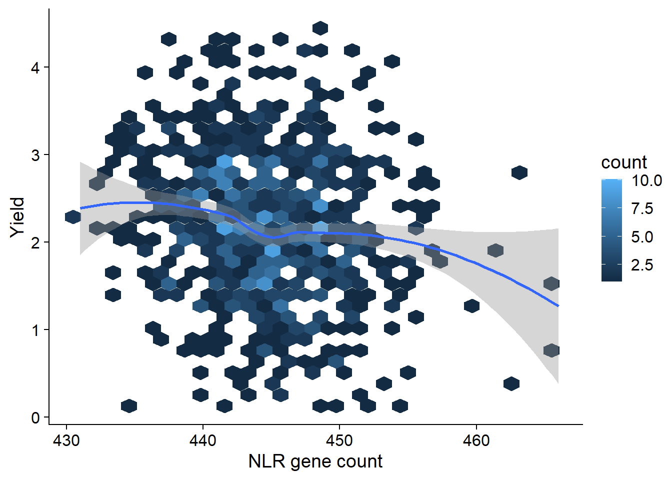
Protein
protein <- read_tsv('./data/protein_phenotype.txt')
protein_join <- left_join(nbs_res_tibb, protein, by=c('names'='Line')) %>% filter(!is.na(Protein))
protein_join %>% ggplot(aes(x=presences, y=Protein)) + geom_hex() + geom_smooth() +
xlab('NLR gene count')
summary(lm(Protein ~ presences, data = protein_join))
Call:
lm(formula = Protein ~ presences, data = protein_join)

Residuals:
     Min       1Q   Median       3Q      Max
-11.8479  -2.1274  -0.3336   1.9959  10.0949

Coefficients:
            Estimate Std. Error t value Pr(>|t|)
(Intercept) -7.98158    7.24125  -1.102    0.271
presences    0.11786    0.01624   7.258 8.07e-13 ***
---
Signif. codes:  0 '***' 0.001 '**' 0.01 '*' 0.05 '.' 0.1 ' ' 1

Residual standard error: 3.106 on 960 degrees of freedom
Multiple R-squared:  0.05203,   Adjusted R-squared:  0.05104
F-statistic: 52.69 on 1 and 960 DF,  p-value: 8.075e-13
Seed weight
Let’s look at seed weight:
seed_weight <- read_tsv('./data/Seed_weight_Phenotype.txt', col_names = c('names', 'wt'))
seed_join <- left_join(nbs_res_tibb, seed_weight) %>% filter(!is.na(wt))
seed_join %>% filter(wt > 5) %>% ggplot(aes(x=presences, y=wt)) + geom_hex() + geom_smooth() +
ylab('Seed weight') +
xlab('NLR gene count')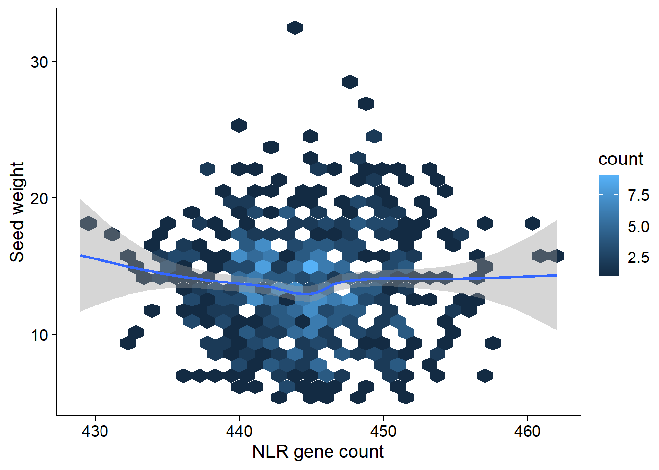
summary(lm(wt ~ presences, data = seed_join))
Call:
lm(formula = wt ~ presences, data = seed_join)

Residuals:
     Min       1Q   Median       3Q      Max
-12.2910  -2.8692   0.1462   2.7771  19.6962

Coefficients:
            Estimate Std. Error t value Pr(>|t|)
(Intercept) 91.40656   14.67990   6.227 8.28e-10 ***
presences   -0.17636    0.03298  -5.348 1.21e-07 ***
---
Signif. codes:  0 '***' 0.001 '**' 0.01 '*' 0.05 '.' 0.1 ' ' 1

Residual standard error: 4.714 on 690 degrees of freedom
Multiple R-squared:  0.0398,    Adjusted R-squared:  0.0384
F-statistic:  28.6 on 1 and 690 DF,  p-value: 1.213e-07
Oil content
And now let’s look at the oil phenotype:
oil <- read_tsv('./data/oil_phenotype.txt')
oil_join <- left_join(nbs_res_tibb, oil, by=c('names'='Line')) %>% filter(!is.na(Oil))
oil_join
# A tibble: 962 x 3
names presences Oil
<chr> <dbl> <dbl>
1 AB-01 445 17.6
2 AB-02 454 16.8
3 BR-24 455 20.6
4 ESS 454 20.9
5 For 448 21
6 HN001 448 23.6
7 HN002 444 18.5
8 HN003 446 17.5
9 HN004 442 18.9
10 HN005 440 15.5
# ... with 952 more rowsoil_join %>% ggplot(aes(x=presences, y=Oil)) + geom_hex() + geom_smooth() +
xlab('NLR gene count')
summary(lm(Oil ~ presences, data = oil_join))
Call:
lm(formula = Oil ~ presences, data = oil_join)

Residuals:
     Min       1Q   Median       3Q      Max
-10.4376  -1.9081   0.4846   2.2401   9.0361

Coefficients:
             Estimate Std. Error t value Pr(>|t|)
(Intercept) 118.03941    7.31646   16.13   <2e-16 ***
presences    -0.22591    0.01641  -13.77   <2e-16 ***
---
Signif. codes:  0 '***' 0.001 '**' 0.01 '*' 0.05 '.' 0.1 ' ' 1

Residual standard error: 3.139 on 960 degrees of freedom
Multiple R-squared:  0.1649,    Adjusted R-squared:  0.1641
F-statistic: 189.6 on 1 and 960 DF,  p-value: < 2.2e-16
OK there are many, many outliers here. Clearly I’ll have to do something fancier - for example, using the first two PCs as covariates might get rid of some of those outliers.
Boxplots per group
Yield
nbs_joined_groups %>%
  filter(!is.na(`Group in violin table`)) %>%
  inner_join(yield, by=c('names'='Line')) %>%
  ggplot(aes(x=`Group in violin table`, y=Yield, fill = `Group in violin table`)) +
  geom_boxplot() +
  scale_fill_manual(values = col_list) +
  theme_minimal_hgrid() +
  theme(axis.text.x = element_text(size=12),
        axis.text.y = element_text(size=12)) +
  geom_signif(comparisons = list(c('Old cultivar', 'Modern cultivar')),
              map_signif_level = T) +
  guides(fill=FALSE) +
  ylab('Protein') +
  xlab('Accession group')
And let’s check the dots:
nbs_joined_groups %>%
  filter(!is.na(`Group in violin table`)) %>%
  inner_join(yield_join, by = 'names') %>%
  ggplot(aes(y=presences.x, x=Yield, color=`Group in violin table`)) +
  geom_point() +
  scale_color_manual(values = col_list) +
  theme_minimal_hgrid() +
  theme(axis.text.x = element_text(size=12),
        axis.text.y = element_text(size=12)) +
  ylab('NLR gene count')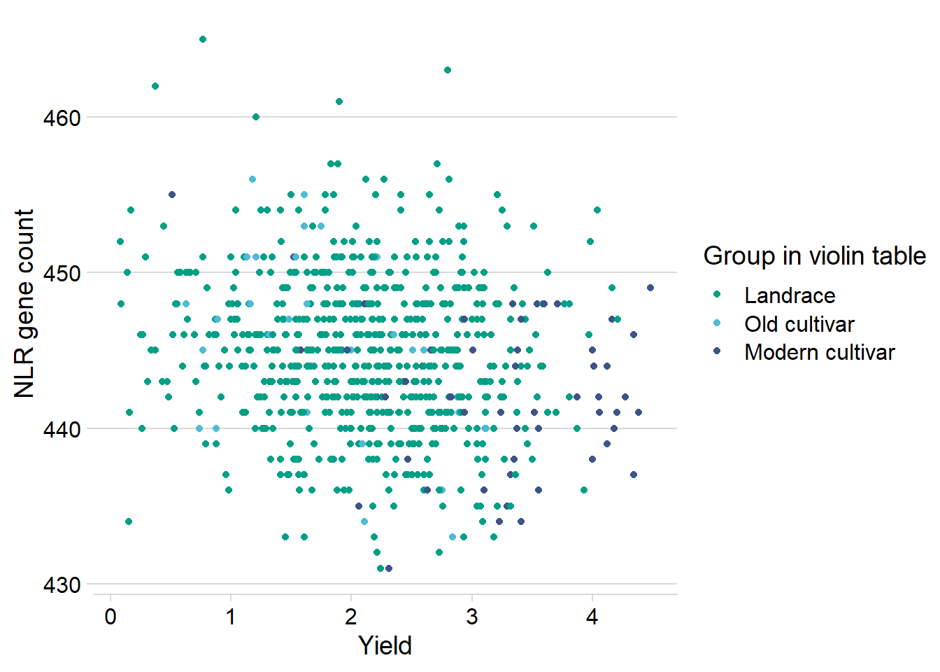
nbs_joined_groups %>%
  filter(!is.na(`Group in violin table`)) %>%
  inner_join(yield_join, by = 'names') %>%
  filter(`Group in violin table` != 'Landrace') %>%
  ggplot(aes(x=presences.x, y=Yield, color=`Group in violin table`)) +
  geom_point() +
  scale_color_manual(values = col_list) +
  theme_minimal_hgrid() +
  geom_smooth() +
  theme(axis.text.x = element_text(size=12),
        axis.text.y = element_text(size=12)) +
  xlab('NLR gene count')
## Protein
protein vs. the four groups:
nbs_joined_groups %>%
  filter(!is.na(`Group in violin table`)) %>%
  inner_join(protein, by=c('names'='Line')) %>%
  ggplot(aes(x=`Group in violin table`, y=Protein, fill = `Group in violin table`)) +
  geom_boxplot() +
  scale_fill_manual(values = col_list) +
  theme_minimal_hgrid() +
  theme(axis.text.x = element_text(size=12),
        axis.text.y = element_text(size=12)) +
  geom_signif(comparisons = list(c('Wild-type', 'Landrace'),
                                 c('Old cultivar', 'Modern cultivar')),
              map_signif_level = T) +
  guides(fill=FALSE) +
  ylab('Protein') +
  xlab('Accession group')
Seed weight
And seed weight:
nbs_joined_groups %>%
  filter(!is.na(`Group in violin table`)) %>%
  inner_join(seed_join) %>%
  ggplot(aes(x=`Group in violin table`, y=wt, fill = `Group in violin table`)) +
  geom_boxplot() +
  scale_fill_manual(values = col_list) +
  theme_minimal_hgrid() +
  theme(axis.text.x = element_text(size=12),
        axis.text.y = element_text(size=12)) +
  geom_signif(comparisons = list(c('Wild-type', 'Landrace'),
                                 c('Old cultivar', 'Modern cultivar')),
              map_signif_level = T) +
  guides(fill=FALSE) +
  ylab('Seed weight') +
  xlab('Accession group')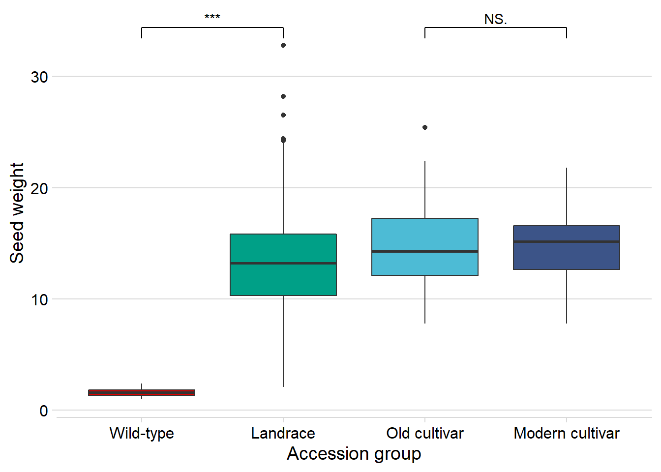
Wow, that’s breeding!
Oil content
And finally, Oil content:
nbs_joined_groups %>%
  filter(!is.na(`Group in violin table`)) %>%
  inner_join(oil_join, by = 'names') %>%
  ggplot(aes(x=`Group in violin table`, y=Oil, fill = `Group in violin table`)) +
  geom_boxplot() +
  scale_fill_manual(values = col_list) +
  theme_minimal_hgrid() +
  theme(axis.text.x = element_text(size=12),
        axis.text.y = element_text(size=12)) +
  geom_signif(comparisons = list(c('Wild-type', 'Landrace'),
                                 c('Old cultivar', 'Modern cultivar')),
              map_signif_level = T) +
  guides(fill=FALSE) +
  ylab('Oil content') +
  xlab('Accession group')
Oha, a single star. That’s p < 0.05!
Let’s redo the above hexplot, but also color the dots by group.
nbs_joined_groups %>%
  filter(!is.na(`Group in violin table`)) %>%
  inner_join(oil_join, by = 'names') %>%
  ggplot(aes(x=presences.x, y=Oil, color=`Group in violin table`)) +
  geom_point() +
  scale_color_manual(values = col_list) +
  theme_minimal_hgrid() +
  theme(axis.text.x = element_text(size=12),
        axis.text.y = element_text(size=12)) +
  xlab('NLR gene count')
Oha, so it’s the wild-types that drag this out a lot.
Let’s remove them and see what it looks like:
nbs_joined_groups %>%
  filter(!is.na(`Group in violin table`)) %>%
  inner_join(oil_join, by = 'names') %>%
  filter(`Group in violin table` %in% c('Old cultivar', 'Modern cultivar')) %>%
  ggplot(aes(x=presences.x, y=Oil, color=`Group in violin table`)) +
  geom_point() +
  scale_color_manual(values = col_list) +
  theme_minimal_hgrid() +
  theme(axis.text.x = element_text(size=12),
        axis.text.y = element_text(size=12)) +
  xlab('NLR gene count') +
  geom_smooth()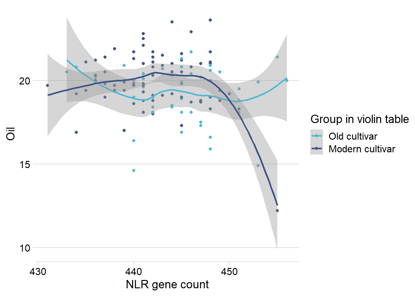
Let’s remove that one outlier:
nbs_joined_groups %>%
  filter(!is.na(`Group in violin table`)) %>%
  inner_join(oil_join, by = 'names') %>%
  filter(`Group in violin table` %in% c('Old cultivar', 'Modern cultivar')) %>%
  filter(Oil > 13) %>%
  ggplot(aes(x=presences.x, y=Oil, color=`Group in violin table`)) +
  geom_point() +
  scale_color_manual(values = col_list) +
  theme_minimal_hgrid() +
  theme(axis.text.x = element_text(size=12),
        axis.text.y = element_text(size=12)) +
  xlab('NLR gene count') +
  geom_smooth()
Does the above oil content boxplot become different if we exclude the one outlier? I’d bet so
nbs_joined_groups %>%
  filter(!is.na(`Group in violin table`)) %>%
  inner_join(oil_join, by = 'names') %>%
  filter(names != 'USB-393') %>%
  ggplot(aes(x=`Group in violin table`, y=Oil, fill = `Group in violin table`)) +
  geom_boxplot() +
  scale_fill_manual(values = col_list) +
  theme_minimal_hgrid() +
  theme(axis.text.x = element_text(size=12),
        axis.text.y = element_text(size=12)) +
  geom_signif(comparisons = list(c('Wild-type', 'Landrace'),
                                 c('Old cultivar', 'Modern cultivar')),
              map_signif_level = T) +
  guides(fill=FALSE) +
  ylab('Oil content') +
  xlab('Accession group')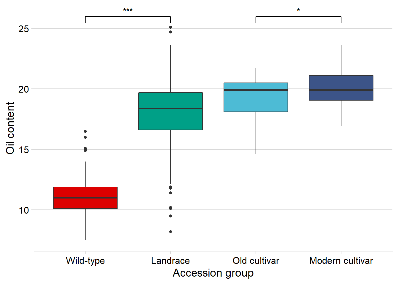
Nope, still significantly higher in modern cultivars!
Mixed modeling
Alright here’s my hypothesis: There’s a link between cultivar status (Old, Wild, Landrace, Modern), r-gene count, and yield, but it’s ‘hidden’ by country differences.
Great tutorial here: https://ourcodingclub.github.io/tutorials/mixed-models
So we’ll have to build some lme4 models!
Oil
nbs_joined_groups$presences2 <- scale(nbs_joined_groups$presences, center=T, scale=T)
hist(nbs_joined_groups$presences2)
oil_nbs_joined_groups <- nbs_joined_groups %>% inner_join(oil_join, by = 'names')
oil_nbs_joined_groups$Oil2 <- scale(oil_nbs_joined_groups$Oil, center=T, scale=T)
basic.lm <- lm(Oil2 ~ presences2, data=oil_nbs_joined_groups)ggplot(oil_nbs_joined_groups, aes(x = presences2, y = Oil2)) +
geom_point() +
geom_smooth(method = "lm")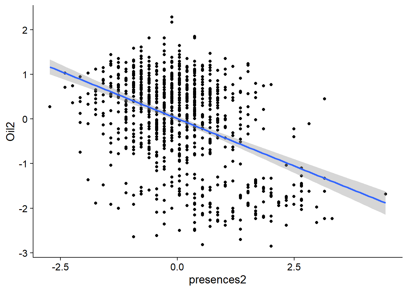
Hm looks messy, you can see two groups
plot(basic.lm, which = 1)
which is confirmed by the messy line
plot(basic.lm, which = 2)
and this garbage qqplot.
So let’s build an lmer model!
mixed.lmer <- lmer(Oil2 ~ presences2 + (1|`Group in violin table`), data=oil_nbs_joined_groups)
summary(mixed.lmer)
Linear mixed model fit by REML. t-tests use Satterthwaite's method [
lmerModLmerTest]
Formula: Oil2 ~ presences2 + (1 | `Group in violin table`)
Data: oil_nbs_joined_groups
REML criterion at convergence: 1872.4
Scaled residuals:
Min 1Q Median 3Q Max
-4.5879 -0.5672 0.0869 0.6631 3.2111
Random effects:
Groups Name Variance Std.Dev.
Group in violin table (Intercept) 1.3349 1.1554
Residual 0.4075 0.6384
Number of obs: 951, groups: Group in violin table, 4
Fixed effects:
Estimate Std. Error df t value Pr(>|t|)
(Intercept) -0.04360 0.57867 2.99844 -0.075 0.9447
presences2 -0.05350 0.02394 947.27006 -2.234 0.0257 *
---
Signif. codes: 0 '***' 0.001 '**' 0.01 '*' 0.05 '.' 0.1 ' ' 1
Correlation of Fixed Effects:
(Intr)
presences2 -0.004So the Variance for Group in violin table is 1.3349, that means it’s 1.3349/(1.3349+0.4075) *100 = 76% of the variance is explained by the four groups!
plot(mixed.lmer)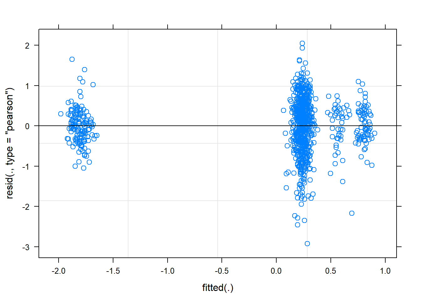
qqnorm(resid(mixed.lmer))
qqline(resid(mixed.lmer))
These still look fairly bad - better than before, but the QQ plot still isn’t on the line.
Let’s quickly check yield too
Yield
yield_nbs_joined_groups <- nbs_joined_groups %>% inner_join(yield_join, by = 'names')
yield_nbs_joined_groups$Yield2 <-scale(yield_nbs_joined_groups$Yield, center=T, scale=T)
mixed.lmer <- lmer(Yield2 ~ presences2 + (1|`Group in violin table`), data=yield_nbs_joined_groups)
summary(mixed.lmer)Linear mixed model fit by REML. t-tests use Satterthwaite's method [
lmerModLmerTest]
Formula: Yield2 ~ presences2 + (1 | `Group in violin table`)
Data: yield_nbs_joined_groups
REML criterion at convergence: 2060.4
Scaled residuals:
Min 1Q Median 3Q Max
-3.1643 -0.6819 0.0316 0.6948 2.8002
Random effects:
Groups Name Variance Std.Dev.
Group in violin table (Intercept) 0.6466 0.8041
Residual 0.8600 0.9274
Number of obs: 761, groups: Group in violin table, 3
Fixed effects:
Estimate Std. Error df t value Pr(>|t|)
(Intercept) 0.23641 0.46910 1.98335 0.504 0.664692
presences2 -0.15364 0.04172 757.46580 -3.683 0.000247 ***
---
Signif. codes: 0 '***' 0.001 '**' 0.01 '*' 0.05 '.' 0.1 ' ' 1
Correlation of Fixed Effects:
(Intr)
presences2 0.025 Percentage explained by breeding group: 0.6466 / (0.6466+0.8600)*100 = 42%
plot(mixed.lmer)
qqnorm(resid(mixed.lmer))
qqline(resid(mixed.lmer))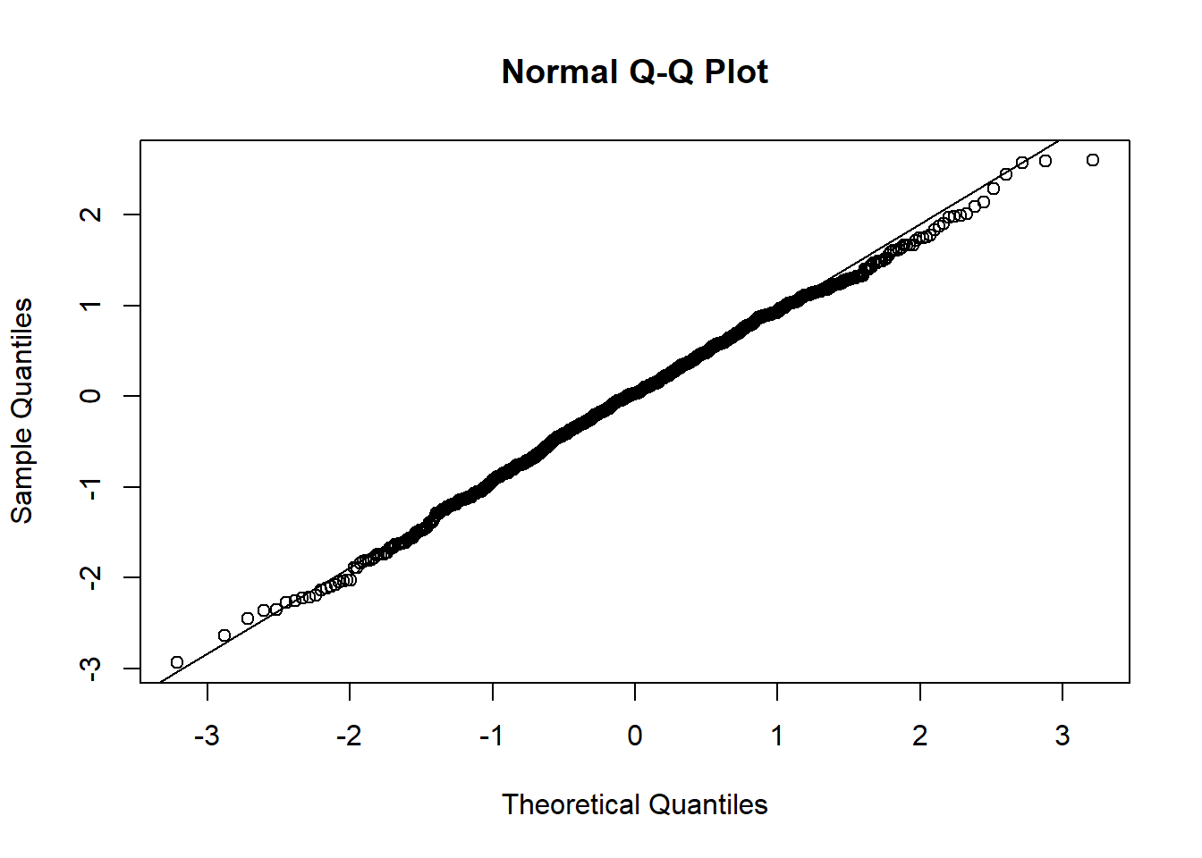
:O
p-value of 0.000247 for the normalised presences while accounting for the breeding group, that’s beautiful.
Adding country
We should also add the country the plant is from as a random effect, that definitely has an influence too (perhaps a stronger one???)
Yield
country <- read_csv('./data/Cultivar_vs_country.csv')

names(country) <- c('names', 'PI-ID', 'Country')

yield_country_nbs_joined_groups <- yield_nbs_joined_groups %>% inner_join(country)
mixed.lmer <- lmer(Yield2 ~ presences2 + (1|`Group in violin table`) + (1|Country), data=yield_country_nbs_joined_groups)
summary(mixed.lmer)Linear mixed model fit by REML. t-tests use Satterthwaite's method [
lmerModLmerTest]
Formula: Yield2 ~ presences2 + (1 | `Group in violin table`) + (1 | Country)
Data: yield_country_nbs_joined_groups
REML criterion at convergence: 1957
Scaled residuals:
Min 1Q Median 3Q Max
-3.09429 -0.56737 0.03072 0.65680 2.89981
Random effects:
Groups Name Variance Std.Dev.
Country (Intercept) 0.3807 0.6170
Group in violin table (Intercept) 0.4178 0.6464
Residual 0.7614 0.8726
Number of obs: 741, groups: Country, 40; Group in violin table, 3
Fixed effects:
Estimate Std. Error df t value Pr(>|t|)
(Intercept) 0.07150 0.40194 2.28533 0.178 0.87336
presences2 -0.11258 0.04116 726.98206 -2.735 0.00639 **
---
Signif. codes: 0 '***' 0.001 '**' 0.01 '*' 0.05 '.' 0.1 ' ' 1
Correlation of Fixed Effects:
(Intr)
presences2 0.051 Nice! Yield is negatively correlated with the number of NLR genes when accounting for breeding group AND country
ggplot(yield_country_nbs_joined_groups, aes(x = presences2, y = Yield2, colour = Country)) +
      facet_wrap(~`Group in violin table`, nrow=2) +   # a panel for each mountain range
      geom_point(alpha = 0.5) +
      theme_classic() +
      geom_line(data = cbind(yield_country_nbs_joined_groups, pred = predict(mixed.lmer)), aes(y = pred), size = 1) +
      theme_minimal_hgrid() +
      theme(legend.position = "none") +
      xlab('Scaled and centered NLR gene count') +
      ylab('Scaled and centered yield')
Some diagnostics:
plot(mixed.lmer)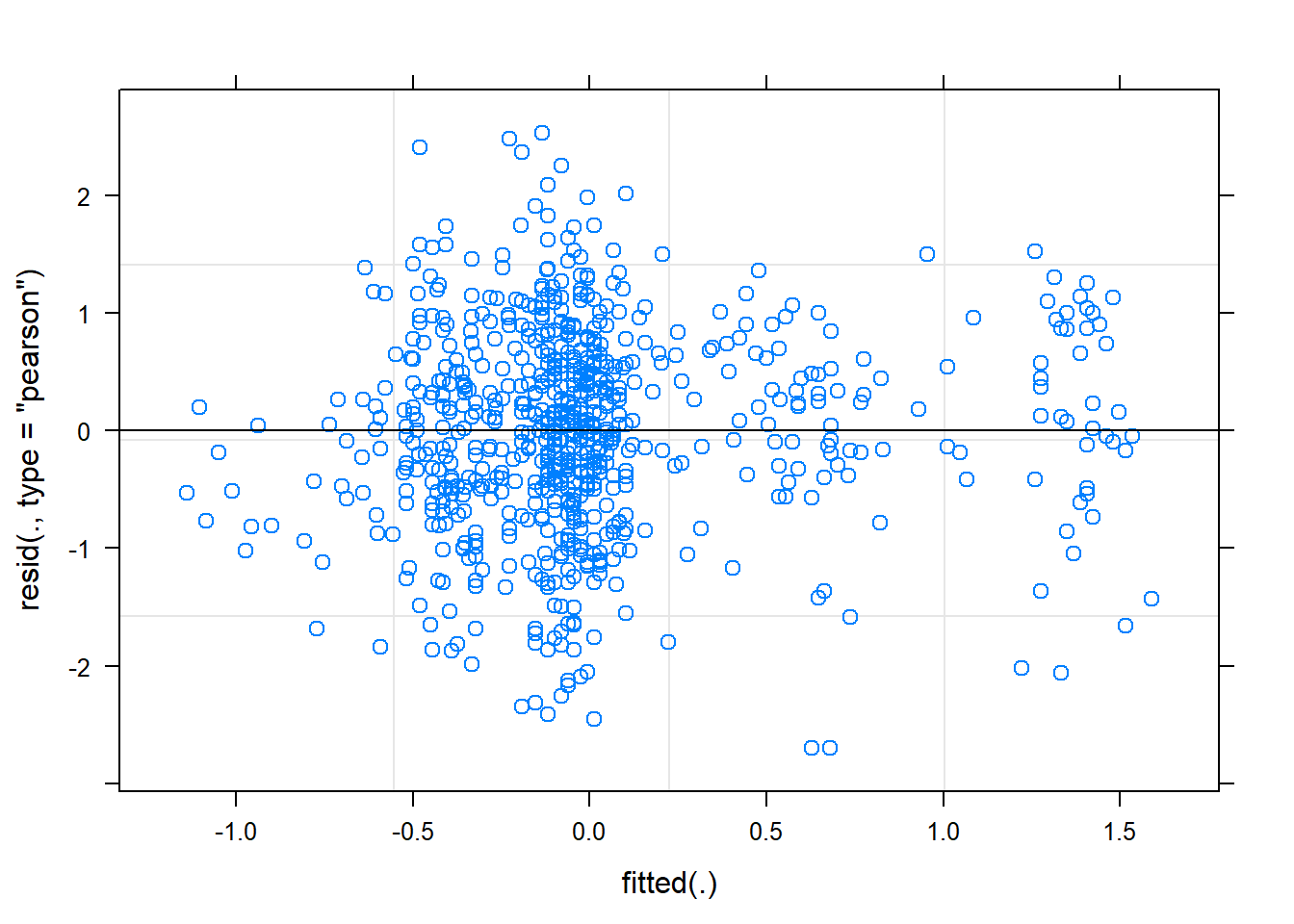
qqnorm(resid(mixed.lmer))
qqline(resid(mixed.lmer))
Hm, the qqplot looks slightly worse than when I use maturity group alone, interesting!
BIG DISCLAIMER: Currently, I treat country and group not as nested variables, they’re independent. I think that is the way it should be in this case but I’m thinking.
Non-normalised yield
Let’s see whether the ‘raw’ values perform the same.
mixed.lmer <- lmer(Yield ~ presences.x + (1|`Group in violin table`) + (1|Country), data=yield_country_nbs_joined_groups)
summary(mixed.lmer)
Linear mixed model fit by REML. t-tests use Satterthwaite's method [
lmerModLmerTest]
Formula: Yield ~ presences.x + (1 | `Group in violin table`) + (1 | Country)
Data: yield_country_nbs_joined_groups
REML criterion at convergence: 1679.6
Scaled residuals:
Min 1Q Median 3Q Max
-3.09429 -0.56737 0.03072 0.65680 2.89981
Random effects:
Groups Name Variance Std.Dev.
Country (Intercept) 0.2602 0.5101
Group in violin table (Intercept) 0.2856 0.5345
Residual 0.5205 0.7215
Number of obs: 741, groups: Country, 40; Group in violin table, 3
Fixed effects:
Estimate Std. Error df t value Pr(>|t|)
(Intercept) 9.011013 2.481360 677.994843 3.631 0.000303 ***
presences.x -0.015192 0.005555 726.982171 -2.735 0.006389 **
---
Signif. codes: 0 '***' 0.001 '**' 0.01 '*' 0.05 '.' 0.1 ' ' 1
Correlation of Fixed Effects:
(Intr)
presences.x -0.991Oh, lower p-values for the intercept
ggplot(yield_country_nbs_joined_groups, aes(x = presences.x, y = Yield, colour = Country)) +
      facet_wrap(~`Group in violin table`, nrow=2) +   # a panel for each mountain range
      geom_point(alpha = 0.5) +
      theme_classic() +
      geom_line(data = cbind(yield_country_nbs_joined_groups, pred = predict(mixed.lmer)), aes(y = pred), size = 1) +
      theme_minimal_hgrid() +
      theme(legend.position = "none") +
      xlab('Raw NLR gene count') +
      ylab('Raw yield')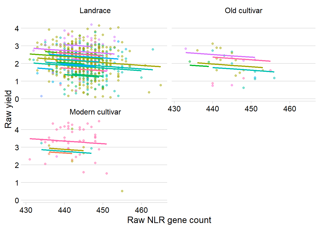
plot(mixed.lmer)
qqnorm(resid(mixed.lmer))
qqline(resid(mixed.lmer))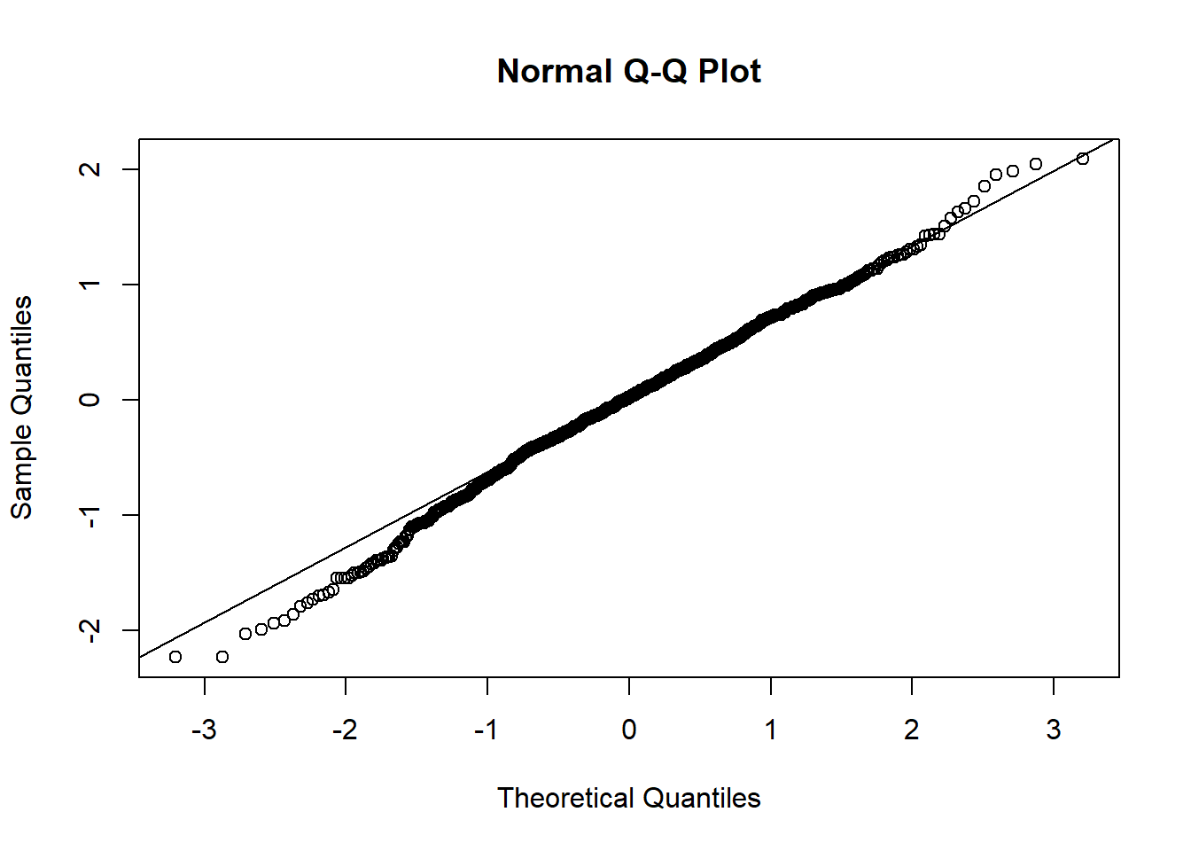
More complex models
If I add random slopes to either groups not much changes, I do get warnings indicating that there’s not much in the data:
mixed.lmer <- lmer(Yield2 ~ presences2 + (1 + presences2|`Group in violin table`) + (1|Country), data=yield_country_nbs_joined_groups)
summary(mixed.lmer)
Linear mixed model fit by REML. t-tests use Satterthwaite's method [
lmerModLmerTest]
Formula: Yield2 ~ presences2 + (1 + presences2 | `Group in violin table`) +
(1 | Country)
Data: yield_country_nbs_joined_groups
REML criterion at convergence: 1954.8
Scaled residuals:
Min 1Q Median 3Q Max
-3.09789 -0.56422 0.04471 0.67067 2.88976
Random effects:
Groups Name Variance Std.Dev. Corr
Country (Intercept) 0.3920 0.6261
Group in violin table (Intercept) 0.3858 0.6211
presences2 0.0310 0.1761 0.30
Residual 0.7564 0.8697
Number of obs: 741, groups: Country, 40; Group in violin table, 3
Fixed effects:
Estimate Std. Error df t value Pr(>|t|)
(Intercept) 0.02964 0.38964 2.29148 0.076 0.945
presences2 -0.22515 0.12370 1.66243 -1.820 0.235
Correlation of Fixed Effects:
(Intr)
presences2 0.269 mixed.lmer <- lmer(Yield2 ~ presences2 + (1|`Group in violin table`) + (1 + presences2|Country), data=yield_country_nbs_joined_groups)
summary(mixed.lmer)Linear mixed model fit by REML. t-tests use Satterthwaite's method [
lmerModLmerTest]
Formula:
Yield2 ~ presences2 + (1 | `Group in violin table`) + (1 + presences2 |
Country)
Data: yield_country_nbs_joined_groups
REML criterion at convergence: 1956.7
Scaled residuals:
Min 1Q Median 3Q Max
-3.10144 -0.57197 0.03398 0.65448 2.90193
Random effects:
Groups Name Variance Std.Dev. Corr
Country (Intercept) 0.399336 0.6319
presences2 0.001875 0.0433 1.00
Group in violin table (Intercept) 0.425089 0.6520
Residual 0.761354 0.8726
Number of obs: 741, groups: Country, 40; Group in violin table, 3
Fixed effects:
Estimate Std. Error df t value Pr(>|t|)
(Intercept) 0.07736 0.40600 2.31158 0.191 0.86434
presences2 -0.11679 0.04281 34.37826 -2.728 0.00997 **
---
Signif. codes: 0 '***' 0.001 '**' 0.01 '*' 0.05 '.' 0.1 ' ' 1
Correlation of Fixed Effects:
(Intr)
presences2 0.116
convergence code: 0
boundary (singular) fit: see ?isSingularOh, a significant p-value, let’s plot plot that and compare with he previous plot:
ggplot(yield_country_nbs_joined_groups, aes(x = presences2, y = Yield2, colour = Country)) +
facet_wrap(~`Group in violin table`, nrow=2) + # a panel for each mountain range
geom_point(alpha = 0.5) +
theme_classic() +
geom_line(data = cbind(yield_country_nbs_joined_groups, pred = predict(mixed.lmer)), aes(y = pred), size = 1) +
theme_minimal_hgrid() +
theme(legend.position = "none") +
xlab('Scaled and centered NLR gene count') +
ylab('Scaled and centered yield')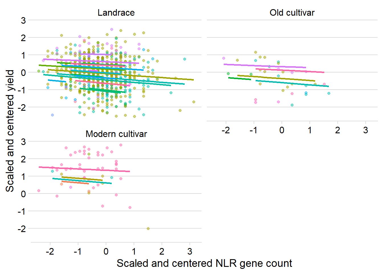 Quite similar, mostly downwards trajectories for each country.
And now both random slopes:
mixed.lmer <- lmer(Yield2 ~ presences2 + (1 + presences2|`Group in violin table`) + (1 + presences2|Country), data=yield_country_nbs_joined_groups)
summary(mixed.lmer)
Linear mixed model fit by REML. t-tests use Satterthwaite's method [
lmerModLmerTest]
Formula: Yield2 ~ presences2 + (1 + presences2 | `Group in violin table`) +
(1 + presences2 | Country)
Data: yield_country_nbs_joined_groups
REML criterion at convergence: 1953.7
Scaled residuals:
Min 1Q Median 3Q Max
-3.11214 -0.56909 0.04459 0.66469 2.91084
Random effects:
Groups Name Variance Std.Dev. Corr
Country (Intercept) 0.42704 0.6535
presences2 0.01045 0.1022 0.81
Group in violin table (Intercept) 0.37523 0.6126
presences2 0.04201 0.2050 0.18
Residual 0.75392 0.8683
Number of obs: 741, groups: Country, 40; Group in violin table, 3
Fixed effects:
Estimate Std. Error df t value Pr(>|t|)
(Intercept) 0.03595 0.38772 2.35869 0.093 0.933
presences2 -0.23848 0.14300 1.96304 -1.668 0.240
Correlation of Fixed Effects:
(Intr)
presences2 0.231 ggplot(yield_country_nbs_joined_groups, aes(x = presences2, y = Yield2, colour = Country)) +
facet_wrap(~`Group in violin table`, nrow=2) + # a panel for each mountain range
geom_point(alpha = 0.5) +
theme_classic() +
geom_line(data = cbind(yield_country_nbs_joined_groups, pred = predict(mixed.lmer)), aes(y = pred), size = 1) +
theme_minimal_hgrid() +
theme(legend.position = "none") +
xlab('Scaled and centered NLR gene count') +
ylab('Scaled and centered yield') Yeah, nah
Oil
oil_country_nbs_joined_groups <- oil_nbs_joined_groups %>% inner_join(country)

mixed.lmer <- lmer(Oil2 ~ presences2 + (1|`Group in violin table`) + (1|Country), data=oil_country_nbs_joined_groups)
summary(mixed.lmer)
Linear mixed model fit by REML. t-tests use Satterthwaite's method [
lmerModLmerTest]
Formula: Oil2 ~ presences2 + (1 | `Group in violin table`) + (1 | Country)
Data: oil_country_nbs_joined_groups
REML criterion at convergence: 1819
Scaled residuals:
Min 1Q Median 3Q Max
-4.5279 -0.5602 0.1003 0.6459 3.2213
Random effects:
Groups Name Variance Std.Dev.
Country (Intercept) 0.07768 0.2787
Group in violin table (Intercept) 1.27074 1.1273
Residual 0.39123 0.6255
Number of obs: 929, groups: Country, 41; Group in violin table, 4
Fixed effects:
Estimate Std. Error df t value Pr(>|t|)
(Intercept) -0.003163 0.568721 3.072981 -0.006 0.996
presences2 -0.036823 0.024149 918.755975 -1.525 0.128
Correlation of Fixed Effects:
(Intr)
presences2 0.004 No significance here.
Protein
protein_nbs_joined_groups <- nbs_joined_groups %>% inner_join(protein_join, by = 'names')
protein_nbs_joined_groups$Protein2 <- scale(protein_nbs_joined_groups$Protein, center=T, scale=T)
protein_country_nbs_joined_groups <- protein_nbs_joined_groups %>% inner_join(country)

mixed.lmer <- lmer(Protein2 ~ presences2 + (1|`Group in violin table`) + (1|Country), data=protein_country_nbs_joined_groups)
summary(mixed.lmer)
Linear mixed model fit by REML. t-tests use Satterthwaite's method [
lmerModLmerTest]
Formula: Protein2 ~ presences2 + (1 | `Group in violin table`) + (1 |
Country)
Data: protein_country_nbs_joined_groups
REML criterion at convergence: 2478.9
Scaled residuals:
Min 1Q Median 3Q Max
-3.5808 -0.6773 -0.0416 0.6268 3.5102
Random effects:
Groups Name Variance Std.Dev.
Country (Intercept) 0.07188 0.2681
Group in violin table (Intercept) 0.28151 0.5306
Residual 0.81194 0.9011
Number of obs: 929, groups: Country, 41; Group in violin table, 4
Fixed effects:
Estimate Std. Error df t value Pr(>|t|)
(Intercept) -0.22283 0.28021 3.35396 -0.795 0.479
presences2 0.04764 0.03456 924.68350 1.378 0.168
Correlation of Fixed Effects:
(Intr)
presences2 0.007 No significance here.
Seed weight
seed_nbs_joined_groups <- nbs_joined_groups %>% inner_join(seed_join, by = 'names')
seed_nbs_joined_groups$wt2 <- scale(seed_nbs_joined_groups$wt, center=T, scale=T)
seed_country_nbs_joined_groups <- seed_nbs_joined_groups %>% inner_join(country)
mixed.lmer <- lmer(wt2 ~ presences2 + (1|`Group in violin table`) + (1|Country), data=seed_country_nbs_joined_groups)
summary(mixed.lmer)
Linear mixed model fit by REML. t-tests use Satterthwaite's method [
lmerModLmerTest]
Formula: wt2 ~ presences2 + (1 | `Group in violin table`) + (1 | Country)
Data: seed_country_nbs_joined_groups
REML criterion at convergence: 1687.6
Scaled residuals:
Min 1Q Median 3Q Max
-2.9631 -0.6170 0.0050 0.5862 4.8133
Random effects:
Groups Name Variance Std.Dev.
Country (Intercept) 0.08584 0.2930
Group in violin table (Intercept) 1.73537 1.3173
Residual 0.70080 0.8371
Number of obs: 664, groups: Country, 38; Group in violin table, 4
Fixed effects:
Estimate Std. Error df t value Pr(>|t|)
(Intercept) -0.36704 0.66678 3.04810 -0.550 0.620
presences2 -0.01035 0.04049 658.64308 -0.256 0.798
Correlation of Fixed Effects:
(Intr)
presences2 0.001 Again, no significance here.
sessionInfo()R version 3.6.3 (2020-02-29)
Platform: x86_64-w64-mingw32/x64 (64-bit)
Running under: Windows 10 x64 (build 17134)
Matrix products: default
locale:
[1] LC_COLLATE=English_Australia.1252 LC_CTYPE=English_Australia.1252
[3] LC_MONETARY=English_Australia.1252 LC_NUMERIC=C
[5] LC_TIME=English_Australia.1252
attached base packages:
[1] stats graphics grDevices utils datasets methods base
other attached packages:
[1] lmerTest_3.1-2 lme4_1.1-21 Matrix_1.2-18
[4] ggforce_0.3.1 ggsignif_0.6.0 cowplot_1.0.0
[7] dabestr_0.3.0 magrittr_1.5 ggsci_2.9
[10] patchwork_1.0.0 forcats_0.5.0 stringr_1.4.0
[13] dplyr_1.0.0 purrr_0.3.4 readr_1.3.1
[16] tidyr_1.1.0 tibble_3.0.2 ggplot2_3.3.2
[19] tidyverse_1.3.0 workflowr_1.6.2.9000
loaded via a namespace (and not attached):
[1] nlme_3.1-148 fs_1.5.0.9000 lubridate_1.7.9
[4] httr_1.4.2 rprojroot_1.3-2 numDeriv_2016.8-1.1
[7] tools_3.6.3 backports_1.1.10 utf8_1.1.4
[10] R6_2.4.1 DBI_1.1.0 mgcv_1.8-31
[13] colorspace_1.4-1 withr_2.2.0 tidyselect_1.1.0
[16] processx_3.4.4 compiler_3.6.3 git2r_0.27.1
[19] cli_2.0.2 rvest_0.3.5 xml2_1.3.2
[22] labeling_0.3 scales_1.1.1 hexbin_1.28.1
[25] callr_3.4.4 digest_0.6.25 minqa_1.2.4
[28] rmarkdown_2.3 pkgconfig_2.0.3 htmltools_0.5.0
[31] dbplyr_1.4.4 rlang_0.4.7 readxl_1.3.1
[34] rstudioapi_0.11 farver_2.0.3 generics_0.0.2
[37] jsonlite_1.7.1 Rcpp_1.0.5 munsell_0.5.0
[40] fansi_0.4.1 lifecycle_0.2.0 stringi_1.5.3
[43] whisker_0.4 yaml_2.2.1 MASS_7.3-51.6
[46] grid_3.6.3 blob_1.2.1 promises_1.1.1
[49] crayon_1.3.4 lattice_0.20-41 haven_2.3.1
[52] splines_3.6.3 hms_0.5.3 knitr_1.29
[55] ps_1.3.4 pillar_1.4.4 boot_1.3-25
[58] reprex_0.3.0 glue_1.4.2 evaluate_0.14
[61] getPass_0.2-2 modelr_0.1.8 vctrs_0.3.1
[64] nloptr_1.2.1 tweenr_1.0.1 httpuv_1.5.4
[67] cellranger_1.1.0 gtable_0.3.0 polyclip_1.10-0
[70] assertthat_0.2.1 xfun_0.17 broom_0.5.6
[73] later_1.1.0.1 ellipsis_0.3.1