ChromHMM
Renee Matthews
2026-02-16
Last updated: 2026-02-16
Checks: 7 0
Knit directory: DXR_continue/
This reproducible R Markdown analysis was created with workflowr (version 1.7.1). The Checks tab describes the reproducibility checks that were applied when the results were created. The Past versions tab lists the development history.
Great! Since the R Markdown file has been committed to the Git repository, you know the exact version of the code that produced these results.
Great job! The global environment was empty. Objects defined in the global environment can affect the analysis in your R Markdown file in unknown ways. For reproduciblity it’s best to always run the code in an empty environment.
The command set.seed(20250701) was run prior to running
the code in the R Markdown file. Setting a seed ensures that any results
that rely on randomness, e.g. subsampling or permutations, are
reproducible.
Great job! Recording the operating system, R version, and package versions is critical for reproducibility.
Nice! There were no cached chunks for this analysis, so you can be confident that you successfully produced the results during this run.
Great job! Using relative paths to the files within your workflowr project makes it easier to run your code on other machines.
Great! You are using Git for version control. Tracking code development and connecting the code version to the results is critical for reproducibility.
The results in this page were generated with repository version ba84b52. See the Past versions tab to see a history of the changes made to the R Markdown and HTML files.
Note that you need to be careful to ensure that all relevant files for
the analysis have been committed to Git prior to generating the results
(you can use wflow_publish or
wflow_git_commit). workflowr only checks the R Markdown
file, but you know if there are other scripts or data files that it
depends on. Below is the status of the Git repository when the results
were generated:
Ignored files:
    Ignored:    .Rhistory
    Ignored:    .Rproj.user/
    Ignored:    data/Bed_exports/
    Ignored:    data/Cormotif_data/
    Ignored:    data/DER_data/
    Ignored:    data/Other_paper_data/
    Ignored:    data/RDS_files/
    Ignored:    data/TE_annotation/
    Ignored:    data/alignment_summary.txt
    Ignored:    data/all_peak_final_dataframe.txt
    Ignored:    data/cell_line_info_.tsv
    Ignored:    data/full_summary_QC_metrics.txt
    Ignored:    data/motif_lists/
    Ignored:    data/number_frag_peaks_summary.txt

Untracked files:
    Untracked:  H3K27ac_all_regions_test.bed
    Untracked:  H3K27ac_consensus_clusters_test.bed
    Untracked:  analysis/GREAT_H3K27ac.Rmd
    Untracked:  analysis/H3K27ac_ChromHMM_FC.Rmd
    Untracked:  analysis/H3K27me3_TE_investigation.Rmd
    Untracked:  analysis/H3K36me3_TE_investigation.Rmd
    Untracked:  analysis/Top2a_Top2b_expression.Rmd
    Untracked:  analysis/maps_and_plots.Rmd
    Untracked:  analysis/proteomics.Rmd
    Untracked:  code/For_john.R
    Untracked:  other_analysis/

Unstaged changes:
    Modified:   analysis/H3K27ac_TE_investigation.Rmd
    Modified:   analysis/H3K27ac_summit_processing.Rmd
    Modified:   analysis/H3K9me3_TE_investigation.Rmd
    Modified:   analysis/H3K9me3_TE_overlap.Rmd
    Modified:   analysis/dual_histone_TE_investigation.Rmd
    Modified:   analysis/summit_files_processing.Rmd
Note that any generated files, e.g. HTML, png, CSS, etc., are not included in this status report because it is ok for generated content to have uncommitted changes.
These are the previous versions of the repository in which changes were
made to the R Markdown (analysis/chromHMM.Rmd) and HTML
(docs/chromHMM.html) files. If you’ve configured a remote
Git repository (see ?wflow_git_remote), click on the
hyperlinks in the table below to view the files as they were in that
past version.
| File | Version | Author | Date | Message |
|---|---|---|---|---|
| Rmd | ba84b52 | reneeisnowhere | 2026-02-16 | updated to TE |
| html | 67b9d8a | reneeisnowhere | 2026-02-16 | Build site. |
| Rmd | fa53545 | reneeisnowhere | 2026-02-16 | adding in magnitude of difference |
| html | a355837 | reneeisnowhere | 2026-02-16 | Build site. |
| Rmd | e5975d2 | reneeisnowhere | 2026-02-16 | adding geometric mean plots |
| html | 3facb4b | reneeisnowhere | 2026-02-02 | Build site. |
| Rmd | c291e10 | reneeisnowhere | 2026-02-02 | adding ATAC data |
| html | 8c900ea | reneeisnowhere | 2026-01-28 | Build site. |
| Rmd | 1a9ab5b | reneeisnowhere | 2026-01-28 | wflow_publish("analysis/chromHMM.Rmd") |
| html | 184a741 | reneeisnowhere | 2026-01-23 | Build site. |
| Rmd | 0db4ed7 | reneeisnowhere | 2026-01-23 | updates |
library(tidyverse)
library(GenomicRanges)
library(plyranges)
library(genomation)
library(readr)
library(rtracklayer)
library(stringr)
library(ggrepel)
library(DT)
library(readxl)
library(ChIPseeker)
library(regioneR)

library(GenomeInfoDb)
This is the AIC/BIC plots genrated to figure out how many states we wanted to use for our modeling of our data:
aic_bic_table_TACC <-read_delim("C:/Users/renee/Other_projects_data/DXR_data/TACC_models/model_selection_summary.tsv",
    delim = "\t", escape_double = FALSE,
    trim_ws = TRUE)

aic_bic_table_TACC %>%
   pivot_longer(cols=c(AIC,BIC), names_to = "test_type",values_to = "calculation") %>%
  ggplot(.,aes(x=States,y=calculation))+
  geom_point()+
  geom_line()+
  facet_wrap(~test_type)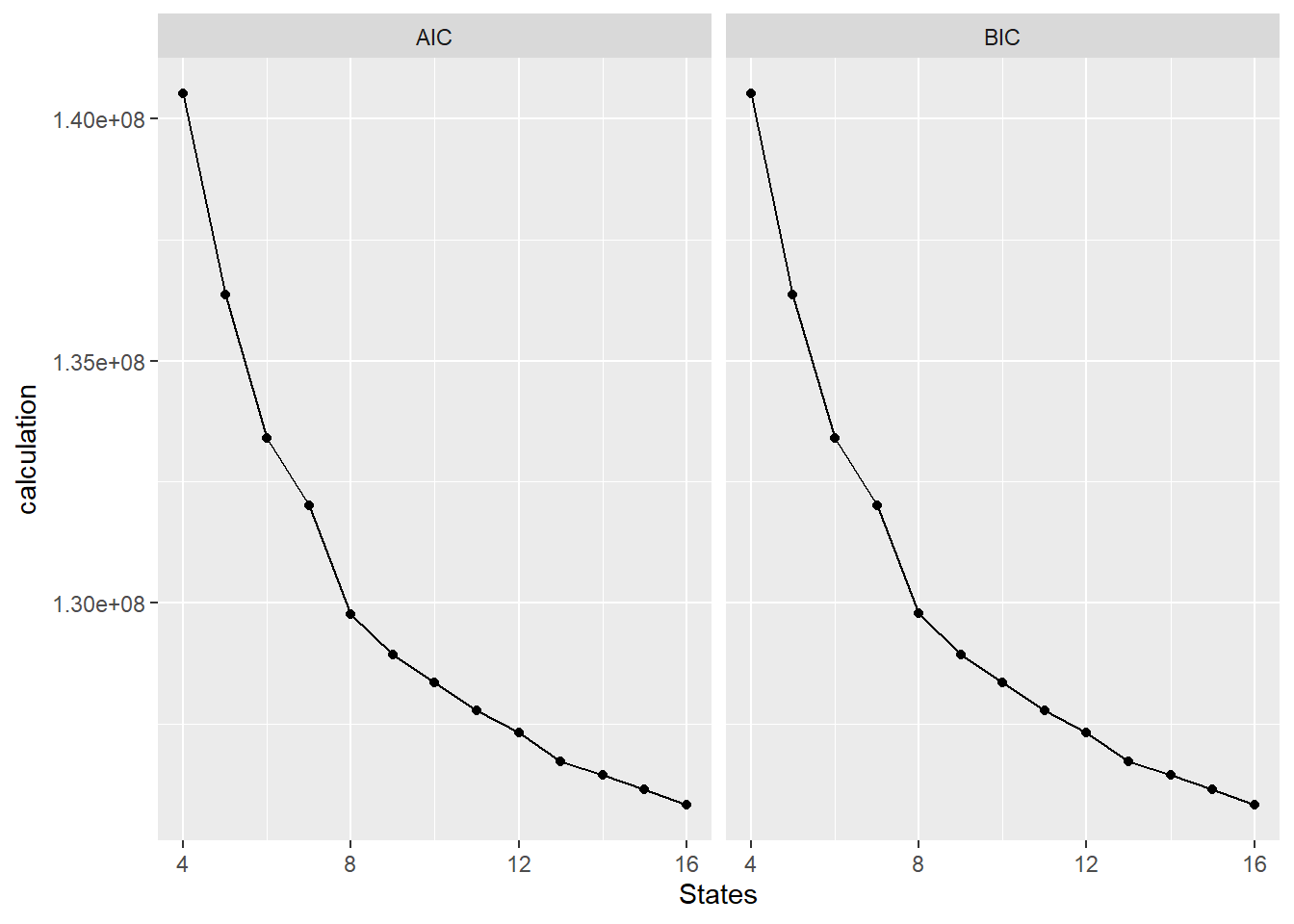
| Version | Author | Date |
|---|---|---|
| 184a741 | reneeisnowhere | 2026-01-23 |
The results point to 16 states yielding the best results.
I ran the models for 16 states and here is the outcome of those results:
Here is the emission table of the results:
emission_16state <- read_delim("C:/Users/renee/Other_projects_data/DXR_data/TACC_models/Chrom_model_16states_final/emissions_16.txt",
    delim = "\t", escape_double = FALSE,
    trim_ws = TRUE)

emission_16state %>%
  mutate(`State (Emission order)`=factor(`State (Emission order)`, levels=c(1:16))) %>%
  pivot_longer(., !`State (Emission order)`, names_to = "Histone",values_to = "emission") %>%
  mutate(Histone=factor(Histone,levels=c("H3K27ac","H3K36me3","H3K27me3","H3K9me3"))) %>%
  ggplot(., aes(x=Histone, y=`State (Emission order)`, fill=emission))+
  geom_tile(color = "grey9",
            lwd = .1,
            linetype = 1)+
     scale_fill_gradient(
  low = "white",
  high = "#08306B",
  limits = c(0, 1),   # <- KEY
  oob = scales::squish,
   na.value = "white",   # <- this sets NAs to white
  name = "scale"
)+
  theme(axis.text.x = element_text(angle = 45, hjust = 1))+
  scale_x_discrete(expand = c(0, 0)) +
scale_y_discrete(expand = c(0, 0), limits = rev)+
  coord_fixed()+
    theme_classic()+
  ggtitle("Emission Parameters")+
  theme(axis.text.x = element_text(angle = 90, hjust = 1))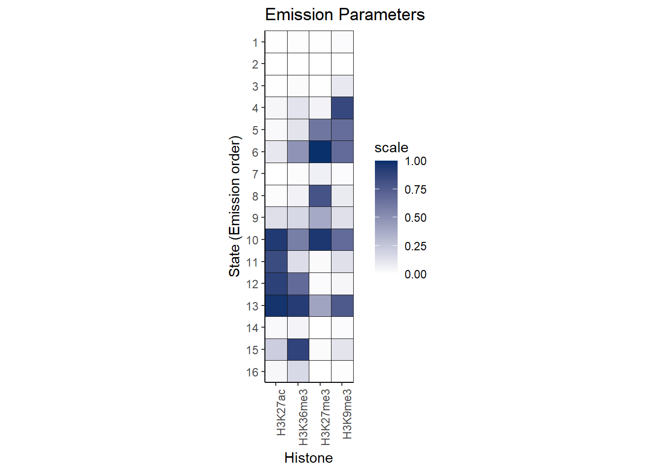
| Version | Author | Date |
|---|---|---|
| 184a741 | reneeisnowhere | 2026-01-23 |
Here is the transition plot of the results:
transition_16state <- read_delim("C:/Users/renee/Other_projects_data/DXR_data/TACC_models/Chrom_model_16states_final/transitions_16.txt",
    delim = "\t", escape_double = FALSE,
    trim_ws = TRUE)

transition_16state %>%
  mutate(`State (from\\to) (Emission order)`=factor(`State (from\\to) (Emission order)`, levels=c(1:16)))%>%
  dplyr::rename(state_from_to=`State (from\\to) (Emission order)`) %>%
  pivot_longer(., !state_from_to, names_to = "States",values_to = "transition") %>%
  mutate(States=factor(States, levels=c(1:16))) %>%

  ggplot(., aes(x=States, y=state_from_to, fill=transition))+
  geom_tile(color = "grey9",
            lwd = .1,
            linetype = 1)+
     scale_fill_gradient(
  low = "white",
  high = "#08306B",
  limits = c(0, 1),   # <- KEY
  oob = scales::squish,
   na.value = "white",   # <- this sets NAs to white
  name = "scale"
)+
  theme(axis.text.x = element_text(angle = 45, hjust = 1))+
  scale_x_discrete(expand = c(0, 0)) +
scale_y_discrete(expand = c(0, 0), limits = rev)+
  coord_fixed()+
    theme_classic()+
  ggtitle("Transition Parameters")+
theme(axis.text.x = element_text(angle = 90, hjust = 1))![]()
| Version | Author | Date |
|---|---|---|
| 184a741 | reneeisnowhere | 2026-01-23 |
Enrichment across the states:
looking at enrichment of Features across the states by each group. This helps with the classification and interpretation of what each state represents.
DOX_24T_full <- read_delim("C:/Users/renee/Other_projects_data/DXR_data/overlap_enrichment_all/rerun_regions/24t_DOX_16.txt",
    delim = "\t", escape_double = FALSE,
    trim_ws = TRUE)%>% mutate(group="DOX_24T")

DOX_24R_full <- read_delim("C:/Users/renee/Other_projects_data/DXR_data/overlap_enrichment_all/rerun_regions/24R_DOX_16.txt",
    delim = "\t", escape_double = FALSE,
    trim_ws = TRUE)%>% mutate(group="DOX_24R")

DOX_144R_full <- read_delim("C:/Users/renee/Other_projects_data/DXR_data/overlap_enrichment_all/rerun_regions/144R_DOX_16.txt",
    delim = "\t", escape_double = FALSE,
    trim_ws = TRUE) %>% mutate(group="DOX_144R")


VEH_24T_full <- read_delim("C:/Users/renee/Other_projects_data/DXR_data/overlap_enrichment_all/rerun_regions/24t_VEH_16.txt",
    delim = "\t", escape_double = FALSE,
    trim_ws = TRUE)%>% mutate(group="VEH_24T")

VEH_24R_full <- read_delim("C:/Users/renee/Other_projects_data/DXR_data/overlap_enrichment_all/rerun_regions/24R_VEH_16.txt",
    delim = "\t", escape_double = FALSE,
    trim_ws = TRUE)%>% mutate(group="VEH_24R")

VEH_144R_full <- read_delim("C:/Users/renee/Other_projects_data/DXR_data/overlap_enrichment_all/rerun_regions/144R_VEH_16.txt",
    delim = "\t", escape_double = FALSE,
    trim_ws = TRUE)%>% mutate(group="VEH_144R")
DOX_24T_gene <- read_delim("C:/Users/renee/Other_projects_data/DXR_data/16-internal-enrichment/24t_DOX_16.txt",
delim = "\t", escape_double = FALSE,
trim_ws = TRUE)%>% mutate(group="DOX_24T")
DOX_24R_gene <- read_delim("C:/Users/renee/Other_projects_data/DXR_data/16-internal-enrichment/24R_DOX_16.txt",
delim = "\t", escape_double = FALSE,
trim_ws = TRUE)%>% mutate(group="DOX_24R")
DOX_144R_gene <- read_delim("C:/Users/renee/Other_projects_data/DXR_data/16-internal-enrichment/144R_DOX_16.txt",
delim = "\t", escape_double = FALSE,
trim_ws = TRUE) %>% mutate(group="DOX_144R")
VEH_24T_gene <- read_delim("C:/Users/renee/Other_projects_data/DXR_data/16-internal-enrichment/24t_VEH_16.txt",
delim = "\t", escape_double = FALSE,
trim_ws = TRUE)%>% mutate(group="VEH_24T")
VEH_24R_gene <- read_delim("C:/Users/renee/Other_projects_data/DXR_data/16-internal-enrichment/24R_VEH_16.txt",
delim = "\t", escape_double = FALSE,
trim_ws = TRUE)%>% mutate(group="VEH_24R")
VEH_144R_gene <- read_delim("C:/Users/renee/Other_projects_data/DXR_data/16-internal-enrichment/144R_VEH_16.txt",
delim = "\t", escape_double = FALSE,
trim_ws = TRUE)%>% mutate(group="VEH_144R")
all_genes_states <-
VEH_144R_gene %>%
bind_rows(DOX_144R_gene) %>%
bind_rows(DOX_24R_gene) %>%
bind_rows(VEH_24R_gene) %>%
bind_rows(DOX_24T_gene) %>%
bind_rows(VEH_24T_gene) DOX_24T_ZFP <- read_delim("C:/Users/renee/Other_projects_data/DXR_data/overlap_enrichment_all/ZFP_run/24t_DOX_16.txt",
delim = "\t", escape_double = FALSE,
trim_ws = TRUE)%>% mutate(group="DOX_24T")
DOX_24R_ZFP <- read_delim("C:/Users/renee/Other_projects_data/DXR_data/overlap_enrichment_all/ZFP_run/24R_DOX_16.txt",
delim = "\t", escape_double = FALSE,
trim_ws = TRUE)%>% mutate(group="DOX_24R")
DOX_144R_ZFP <- read_delim("C:/Users/renee/Other_projects_data/DXR_data/overlap_enrichment_all/ZFP_run/144R_DOX_16.txt",
delim = "\t", escape_double = FALSE,
trim_ws = TRUE) %>% mutate(group="DOX_144R")
VEH_24T_ZFP <- read_delim("C:/Users/renee/Other_projects_data/DXR_data/overlap_enrichment_all/ZFP_run/24t_VEH_16.txt",
delim = "\t", escape_double = FALSE,
trim_ws = TRUE)%>% mutate(group="VEH_24T")
VEH_24R_ZFP <- read_delim("C:/Users/renee/Other_projects_data/DXR_data/overlap_enrichment_all/ZFP_run/24R_VEH_16.txt",
delim = "\t", escape_double = FALSE,
trim_ws = TRUE)%>% mutate(group="VEH_24R")
VEH_144R_ZFP <- read_delim("C:/Users/renee/Other_projects_data/DXR_data/overlap_enrichment_all/ZFP_run/144R_VEH_16.txt",
delim = "\t", escape_double = FALSE,
trim_ws = TRUE)%>% mutate(group="VEH_144R")
all_ZFPs_states <-
VEH_144R_ZFP %>%
bind_rows(DOX_144R_ZFP) %>%
bind_rows(DOX_24R_ZFP) %>%
bind_rows(VEH_24R_ZFP) %>%
bind_rows(DOX_24T_ZFP) %>%
bind_rows(VEH_24T_ZFP)
just_ZFP <- all_ZFPs_states[,c("State (Emission order)","ZFP_proteins.bed","group")]
just_ZFP %>%
dplyr::filter(`State (Emission order)` !="Base")# A tibble: 96 × 3
`State (Emission order)` ZFP_proteins.bed group
<chr> <dbl> <chr>
1 E2 0.212 VEH_144R
2 E1 0.712 VEH_144R
3 E4 2.06 VEH_144R
4 E3 1.82 VEH_144R
5 E9 0.745 VEH_144R
6 E7 0.649 VEH_144R
7 E8 0.774 VEH_144R
8 E6 0.764 VEH_144R
9 E5 0.561 VEH_144R
10 E11 1.64 VEH_144R
# ℹ 86 more rowsDOX_24T_ATAC <- read_delim("C:/Users/renee/Other_projects_data/DXR_data/overlap_enrichment_all/ATAC_run/24t_DOX_16.txt",
delim = "\t", escape_double = FALSE,
trim_ws = TRUE)%>% mutate(group="DOX_24T")
DOX_24R_ATAC <- read_delim("C:/Users/renee/Other_projects_data/DXR_data/overlap_enrichment_all/ATAC_run/24R_DOX_16.txt",
delim = "\t", escape_double = FALSE,
trim_ws = TRUE)%>% mutate(group="DOX_24R")
DOX_144R_ATAC <- read_delim("C:/Users/renee/Other_projects_data/DXR_data/overlap_enrichment_all/ATAC_run/144R_DOX_16.txt",
delim = "\t", escape_double = FALSE,
trim_ws = TRUE) %>% mutate(group="DOX_144R")
VEH_24T_ATAC <- read_delim("C:/Users/renee/Other_projects_data/DXR_data/overlap_enrichment_all/ATAC_run/24t_VEH_16.txt",
delim = "\t", escape_double = FALSE,
trim_ws = TRUE)%>% mutate(group="VEH_24T")
VEH_24R_ATAC <- read_delim("C:/Users/renee/Other_projects_data/DXR_data/overlap_enrichment_all/ATAC_run/24R_VEH_16.txt",
delim = "\t", escape_double = FALSE,
trim_ws = TRUE)%>% mutate(group="VEH_24R")
VEH_144R_ATAC <- read_delim("C:/Users/renee/Other_projects_data/DXR_data/overlap_enrichment_all/ATAC_run/144R_VEH_16.txt",
delim = "\t", escape_double = FALSE,
trim_ws = TRUE)%>% mutate(group="VEH_144R")
all_ATAC_states <-
VEH_144R_ATAC %>%
bind_rows(DOX_144R_ATAC) %>%
bind_rows(DOX_24R_ATAC) %>%
bind_rows(VEH_24R_ATAC) %>%
bind_rows(DOX_24T_ATAC) %>%
bind_rows(VEH_24T_ATAC) all_files_states <-
VEH_144R_full %>%
bind_rows(DOX_144R_full) %>%
bind_rows(DOX_24R_full) %>%
bind_rows(VEH_24R_full) %>%
bind_rows(DOX_24T_full) %>%
bind_rows(VEH_24T_full)
long_file <- all_files_states %>%
dplyr::select(`State (Emission order)`,
`Genome %`,
`GRCh38-cCREs.bed`,
`SCREEN_hg38_CA-CTCF.bed`:SCREEN_hg38_pELS.bed,
Set_1_H3K27ac_ROI.bed:Set_3_H3K27ac_ROI.bed,
all_H3K27ac_H3K27ac_ROI.bed,
LINE_rptmasker.bed,
SINE_rptmasker.bed,
LTR_rptmasker.bed,
DNA_rptmasker.bed,
Retroposon_rptmasker.bed,
RC_rptmasker.bed,
Low_complexity_rptmasker.bed,
RNA_rptmasker.bed,
Satellite_rptmasker.bed,
Simple_repeat_rptmasker.bed,
Unknown_rptmasker.bed,
rRNA_rptmasker.bed:group) %>%
mutate(`State (Emission order)`=factor(`State (Emission order)`, levels = c(paste0("E", 1:16),"Base"))) %>%
dplyr::filter(`State (Emission order)` != "Base") %>%
pivot_longer(., cols=!c(`State (Emission order)`,group), names_to = "Identity",values_to = "Fold_enrichment") %>%
mutate(Identity=str_remove(Identity,".bed")) %>%
mutate(Identity=factor(Identity,
levels=c("Genome %",
"GRCh38-cCREs",
"SCREEN_hg38_CA-CTCF",
"SCREEN_hg38_CA-H3K4me3",
"SCREEN_hg38_CA-TF",
"SCREEN_hg38_CA",
"SCREEN_hg38_PLS",
"SCREEN_hg38_TF",
"SCREEN_hg38_pELS",
"SCREEN_hg38_dELS",
"all_H3K27ac_H3K27ac_ROI",
"Set_1_H3K27ac_ROI",
"Set_2_H3K27ac_ROI",
"Set_3_H3K27ac_ROI",
"LINE_rptmasker",
"SINE_rptmasker",
"LTR_rptmasker",
"DNA_rptmasker",
"Retroposon_rptmasker",
"RC_rptmasker",
"Low_complexity_rptmasker",
"RNA_rptmasker",
"Satellite_rptmasker",
"Simple_repeat_rptmasker",
"Unknown_rptmasker",
"rRNA_rptmasker",
"scRNA_rptmasker",
"snRNA_rptmasker",
"srpRNA_rptmasker",
"tRNA_rptmasker"))) %>%
mutate(group=factor(group,levels=c("VEH_24T","VEH_24R","VEH_144R","DOX_24T", "DOX_24R", "DOX_144R")))# columns to pivot (exclude ID columns)
id_cols <- c("State (Emission order)", "group")
all_genes_states_long <-
all_genes_states %>%
mutate(`State (Emission order)`=paste0("E",`State (Emission order)`)) %>%
left_join(just_ZFP) %>%
mutate(`State (Emission order)` = factor(`State (Emission order)`,
levels = c(paste0("E",1:16),"EBase"))) %>%
filter(`State (Emission order)` != "EBase") %>%
pivot_longer(
cols = -all_of(id_cols),
names_to = "Identity",
values_to = "Fold_enrichment"
) %>%
# preserve original order
mutate(Identity = factor(Identity, levels =c( names(all_genes_states)[!names(all_genes_states) %in% id_cols],"ZFP_proteins.bed"))) %>%
# create cleaned label for plotting
mutate(Identity_label = case_when(
str_detect(Identity, "\\.hg38\\.bed\\.gz$") ~ str_remove(Identity, "\\.hg38\\.bed\\.gz$"),
str_detect(Identity, "\\.bed$") ~ str_remove(Identity, "\\.bed$"),
TRUE ~ Identity # keep everything else unchanged
),
group = factor(group,
levels = c("VEH_24T","VEH_24R","VEH_144R",
"DOX_24T","DOX_24R","DOX_144R")))
final_order <- unique(all_genes_states_long$Identity_label)
all_genes_states_long <- all_genes_states_long %>%
mutate(Identity_label=factor(Identity_label,levels=final_order))Looking a genomic features:
all_genes_states_long %>%
  group_by(Identity) %>%   # i.e. per annotation column
  mutate(
    FE_min = min(Fold_enrichment, na.rm = TRUE),
    FE_max = max(Fold_enrichment, na.rm = TRUE),
    chromhmm_scaled = (Fold_enrichment - FE_min) / (FE_max - FE_min)
  ) %>%
    ggplot(.,aes(x=Identity_label,y=`State (Emission order)`, fill=chromhmm_scaled))+
  geom_tile(color = "grey9",
            lwd = .1,
            linetype = 1)+
     scale_fill_gradient(
  low = "white",
  high = "#08306B",
  limits = c(0, 1),   # <- KEY
  oob = scales::squish,
   na.value = "white",   # <- this sets NAs to white
  name = "transformed scale"
)+
  theme(axis.text.x = element_text(angle = 45, hjust = 1))+
  facet_wrap(~group, nrow=1, ncol=6)+
    scale_y_discrete(limits=rev)+
  ggtitle("Genic region enrichment across states")+
  coord_fixed()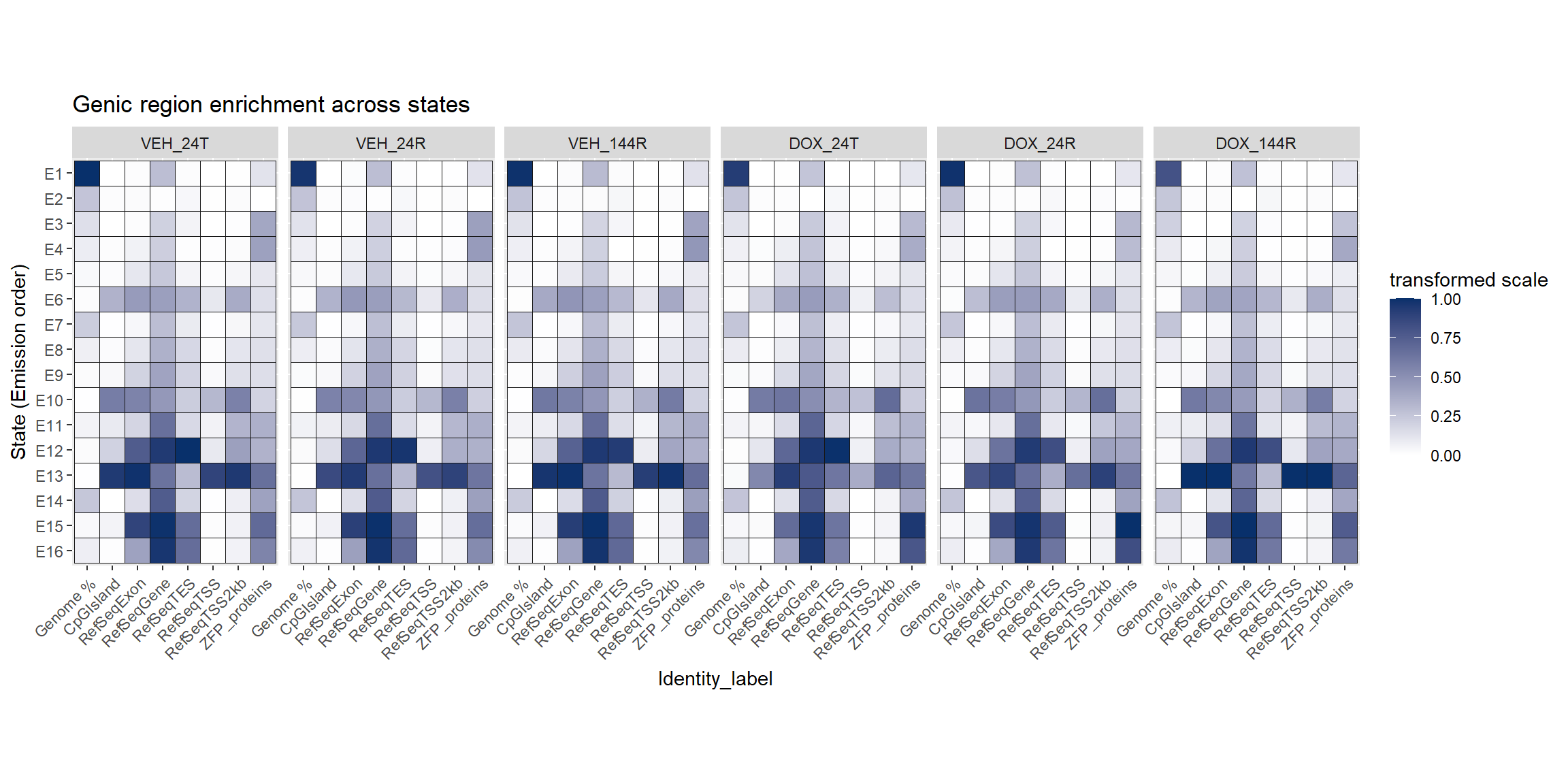
| Version | Author | Date |
|---|---|---|
| 184a741 | reneeisnowhere | 2026-01-23 |
The genic enrichment across states plots shows the exact enrichment across each condtion, however, for summary purposes, I wish to know the general enrichment from all conditions. I will take the geometric mean across DOX and VEH conditions (and all conditions) at each timepoint for each state and identity ( in this case for the CpGIslands, Exons, genes, TESs and TSS etc..). This treats the fold-change enrichment and depletion symmetrically about 1 because enrichment behaves multiplicatively because it is already a ratio. I am only using this to determine which states are constitutively TSS-enriched, with are CPG-biased, which are ZFP biased etc…
geom_mean_df <- all_genes_states_long %>%
  group_by(Identity, Identity_label, `State (Emission order)`) %>%
  summarize(geom_FE = exp(mean(log(Fold_enrichment + 1e-6), na.rm = TRUE)),
    .groups = "drop") %>%
  group_by(Identity) %>%
             mutate(
    FE_min = min(geom_FE, na.rm = TRUE),
    FE_max = max(geom_FE, na.rm = TRUE),
    chromhmm_scaled = (geom_FE - FE_min) / (FE_max - FE_min))

  ggplot(geom_mean_df,aes(x=Identity_label,y=`State (Emission order)`, fill=chromhmm_scaled))+
  geom_tile(color = "grey9",
            lwd = .1,
            linetype = 1)+
     scale_fill_gradient(
  low = "white",
  high = "#08306B",
  limits = c(0, 1),   # <- KEY
  oob = scales::squish,
   na.value = "white",   # <- this sets NAs to white
  name = "transformed scale"
)+
  theme(axis.text.x = element_text(angle = 45, hjust = 1))+

    scale_y_discrete(limits=rev)+
  ggtitle("Genic region relative enrichment pattern across conditions\n (geometric mean)")+
  coord_fixed()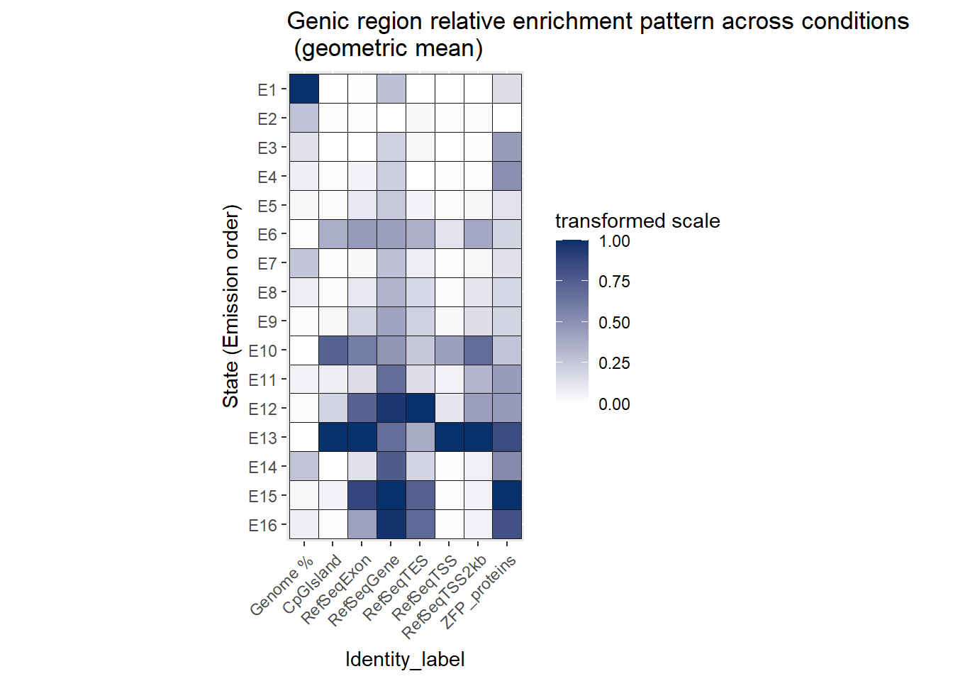
| Version | Author | Date |
|---|---|---|
| a355837 | reneeisnowhere | 2026-02-16 |
geom_mean_df <- geom_mean_df %>%  mutate(log2_FE = log2(geom_FE))

ggplot(geom_mean_df,
       aes(x = Identity_label,
           y = `State (Emission order)`,
           fill = log2_FE)) +

  geom_tile(color = "grey9", linewidth = 0.1) +

  scale_fill_gradient2(
    low = "darkgreen",
    mid = "white",
    high = "#08306B",
    midpoint = 0,
    name = "log2(Fold Enrichment)"
  ) +

  scale_y_discrete(limits = rev) +

  theme_minimal() +
  theme(
    axis.text.x = element_text(angle = 45, hjust = 1)
  ) +

  ggtitle("Geometric Mean ChromHMM Enrichment Across Conditions")+
  coord_fixed()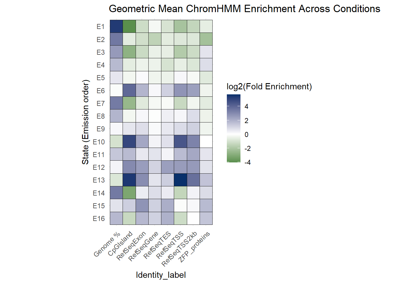
| Version | Author | Date |
|---|---|---|
| a355837 | reneeisnowhere | 2026-02-16 |
Now I want to look at the change of log2 Foldenrichment of DOX -VEH at each timepoint
df_1 <- all_genes_states_long %>%
  mutate(log2_FE = log2(Fold_enrichment + 1e-6)) %>%
  separate(group, into = c("trt","time"), remove = FALSE)

delta_df_1 <- df_1 %>%
  group_by(time, Identity, Identity_label, `State (Emission order)`) %>%
  summarise(
    delta_log2FE =
      log2_FE[trt == "DOX"] -
      log2_FE[trt == "VEH"],
    .groups = "drop") %>%
  mutate(time=factor(time, levels=c("24T","24R","144R")))

ggplot(delta_df_1,
       aes(x = Identity_label,
           y = `State (Emission order)`,
           fill = delta_log2FE)) +

  geom_tile(color = "grey9", linewidth = 0.1) +

  scale_fill_gradient2(
    low = "#67001F",
    mid = "white",
    high = "#053061",
    midpoint = 0,
    name = "log2(DOX / VEH)"
  ) +

  facet_wrap(~time, nrow = 1) +

  scale_y_discrete(limits = rev) +

  theme_minimal() +
  theme(axis.text.x = element_text(angle = 45, hjust = 1))+
  ggtitle("Delta of log2(DOX/VEH) at each timepoint")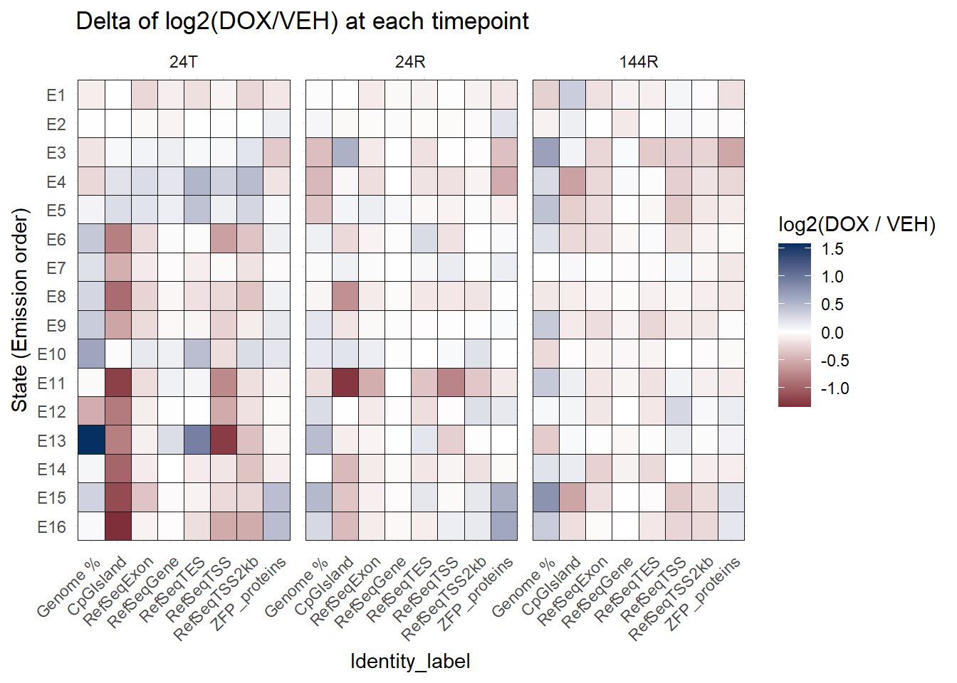
| Version | Author | Date |
|---|---|---|
| 67b9d8a | reneeisnowhere | 2026-02-16 |
Enhancer plot
long_file %>%
  dplyr::filter(stringr::str_detect(Identity, "SCREEN")) %>%
   group_by(Identity) %>%   # i.e. per annotation column
  mutate(
    FE_min = min(Fold_enrichment, na.rm = TRUE),
    FE_max = max(Fold_enrichment, na.rm = TRUE),
    chromhmm_scaled = (Fold_enrichment - FE_min) / (FE_max - FE_min)
  ) %>%
    ggplot(.,aes(x=Identity,y=`State (Emission order)`, fill=chromhmm_scaled))+
  geom_tile(color = "grey9",
            lwd = .1,
            linetype = 1)+
     scale_fill_gradient(
  low = "white",
  high = "#08306B",
  limits = c(0, 1),   # <- KEY
  oob = scales::squish,
   na.value = "white",   # <- this sets NAs to white
  name = "transformed scale"
)+
  theme(axis.text.x = element_text(angle = 45, hjust = 1))+
  facet_wrap(~group, nrow=1, ncol=6)+
    scale_y_discrete(limits=rev)+
  ggtitle("All Enhancer types enrichment across states")+
  coord_fixed()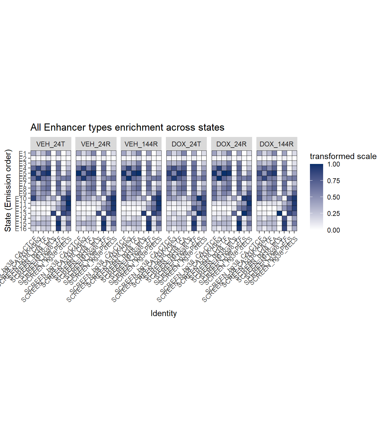
Cormotif set enrichment across states
Each Histone will have slices of their own states. Here are all sets next to all states
order <- c("Genome %",
"all_H3K27ac_H3K27ac_ROI.bed",
"Set_1_H3K27ac_ROI.bed" ,
"Set_2_H3K27ac_ROI.bed",
"Set_3_H3K27ac_ROI.bed",
"all_H3K36me3_regions_H3K36me3_ROI.bed",
"Set_1_H3K36me3_ROI.bed",
"Set_2_H3K36me3_ROI.bed",
"all_H3K27me3_regions_H3K27me3_ROI.bed",
"Set_1_H3K27me3_ROI.bed",
"Set_2_H3K27me3_ROI.bed" ,
"all_H3K9me3_regions_H3K9me3_ROI.bed",
"Set_1_H3K9me3_ROI.bed",
"Set_2_H3K9me3_ROI.bed",
"Set_3_H3K9me3_ROI.bed" ,
"ZFP_proteins.bed")

all_ZFPs_states %>%
  mutate(
    `State (Emission order)` = as.character(`State (Emission order)`),
    `State (Emission order)` = case_when(
      `State (Emission order)` %in% as.character(1:16) ~ paste0("E", `State (Emission order)`),
      TRUE ~ `State (Emission order)`)) %>%
  mutate(`State (Emission order)` = factor(`State (Emission order)`,
                                           levels = c(paste0("E",1:16), "Base"))) %>%
  filter(`State (Emission order)` != "Base") %>%
  pivot_longer(., -c(`State (Emission order)`,group), names_to = "Identity", values_to="Fold_enrichment") %>%
   mutate(group=factor(group,levels=c("VEH_24T","VEH_24R","VEH_144R","DOX_24T", "DOX_24R", "DOX_144R"))) %>%
  mutate(Identity=factor(Identity, levels=order)) %>%
  dplyr::filter(Identity!="ZFP_proteins.bed") %>%
  group_by(Identity) %>%   # i.e. per annotation column
  mutate(
    FE_min = min(Fold_enrichment, na.rm = TRUE),
    FE_max = max(Fold_enrichment, na.rm = TRUE),
    chromhmm_scaled = (Fold_enrichment - FE_min) / (FE_max - FE_min)
  ) %>%
    ggplot(.,aes(x=Identity,y=`State (Emission order)`, fill=chromhmm_scaled))+
  geom_tile(color = "grey9",
            lwd = .1,
            linetype = 1)+
     scale_fill_gradient(
  low = "white",
  high = "#08306B",
  limits = c(0, 1),   # <- KEY
  oob = scales::squish,
   na.value = "white",   # <- this sets NAs to white
  name = "transformed scale"
)+
  theme(axis.text.x = element_text(angle = 45, hjust = 1))+
  facet_wrap(~group, nrow=2, ncol=3)+
    scale_y_discrete(limits=rev)+
  ggtitle("Cormotif across states")+
  coord_fixed()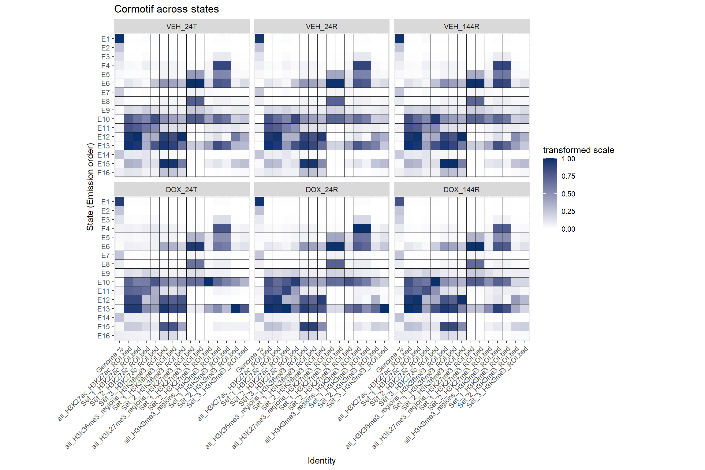
Adding annotation to states
States_anno <- data.frame("State"=c(paste0("E",1:16)),
"Name"=c("Heterochromatin",
"Quiescent_Low_Coverage",
"Repressed_Heterochromatin",
"Repressed_ZNF_regions",
"Strong_Polycomb_Repressed",
 "Bivalent_Enhancer",
"Bivalent_Poised_TSS1",
"Bivalent_Poised_TSS2",
 "Weak_Genic_Enhancer",
 "Strong_Genic_Enhancer1",
 "Active_Proximal_Enhancer",
  "Strong_Genic_Enhancer2",
 "Active_TSS",
 "Very_Weak_Transcription",
 "Genic_Strong_Transcription",
 "Genic_Weak_Transcription"))

# SOIs <- c("E4","E10","E11","E12","E13")
long_file %>%
dplyr::filter(stringr::str_detect(Identity, "_rptmasker")) %>%
mutate(rpt=case_when(Identity=="LINE_rptmasker"~"LINE",
Identity=="SINE_rptmasker"~"SINE",
Identity=="LTR_rptmasker"~"LTR",
Identity=="DNA_rptmasker"~"DNA",
Identity=="Retroposon_rptmasker"~"SVA",
TRUE~"Other")) %>%
dplyr::filter(rpt != "Other") %>%
group_by(Identity) %>% # i.e. per annotation column
mutate(
FE_min = min(Fold_enrichment, na.rm = TRUE),
FE_max = max(Fold_enrichment, na.rm = TRUE),
chromhmm_scaled = (Fold_enrichment - FE_min) / (FE_max - FE_min)
) %>%
ggplot(.,aes(x=rpt,y=`State (Emission order)`, fill=chromhmm_scaled))+
geom_tile(color = "grey9",
lwd = .1,
linetype = 1)+
scale_fill_gradient(
low = "white",
high = "#08306B",
limits = c(0, 1), # <- KEY
oob = scales::squish,
na.value = "white", # <- this sets NAs to white
name = "transformed scale"
)+
theme(axis.text.x = element_text(angle = 45, hjust = 1))+
facet_wrap(~group, nrow=2, ncol=3)+
scale_y_discrete(limits=rev)+
ggtitle("Transposable elements across states")+
coord_fixed()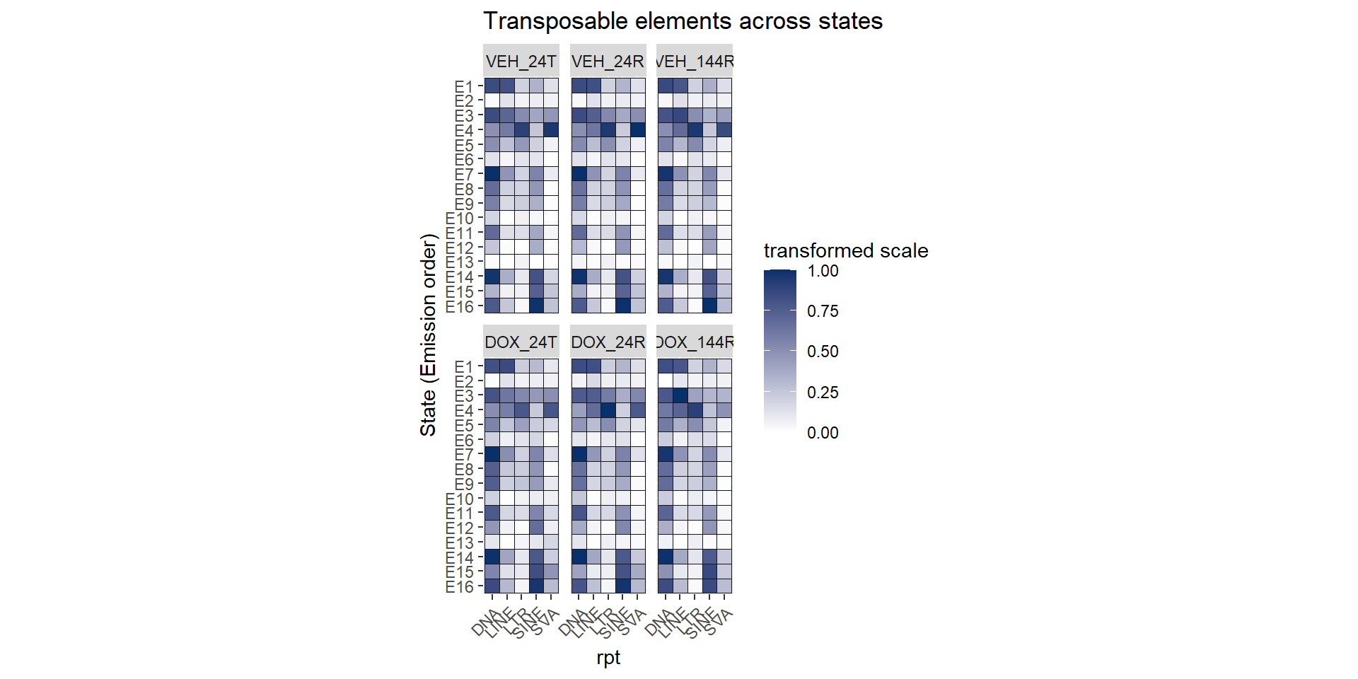
| Version | Author | Date |
|---|---|---|
| 8c900ea | reneeisnowhere | 2026-01-28 |
Looking at Delta TEs
Now using the delta of DOX-VEH (the log2 FE of each) and plotting the states
delta_TE_df <- long_file %>%
  dplyr::filter(stringr::str_detect(Identity, "_rptmasker")) %>%
  mutate(rpt=case_when(Identity=="LINE_rptmasker"~"LINE",
                       Identity=="SINE_rptmasker"~"SINE",
                       Identity=="LTR_rptmasker"~"LTR",
                       Identity=="DNA_rptmasker"~"DNA",
                       Identity=="Retroposon_rptmasker"~"SVA",
                       TRUE~"Other")) %>%
  mutate(log2_FE = log2(Fold_enrichment + 1e-6)) %>%
  separate(group, into = c("trt","time"), remove = FALSE) %>%
  dplyr::filter(rpt != "Other") %>%
  group_by(time,  rpt, `State (Emission order)`) %>%
  summarise(
    delta_log2FE =
      log2_FE[trt == "DOX"] -
      log2_FE[trt == "VEH"],
    .groups = "drop") %>%
  mutate(time=factor(time, levels=c("24T","24R","144R")))


ggplot(delta_TE_df ,
       aes(x = time,
           y = `State (Emission order)`,
           fill = delta_log2FE)) +
  geom_tile(color = "grey20", linewidth = 0.2) +

  scale_fill_gradient2(
    low = "#B2182B",   # Decrease
    mid = "white",     # No change
    high = "#2166AC",  # Increase
    midpoint = 0,
    limits = c(-2.5, 2.5),
    name = "Δ log2(FE)\n(DOX - VEH)"
  ) +

  labs(
    x = "Timepoint",
    y = "ChromHMM State",
    title = "TE Enrichment Changes After DNA Damage"
  ) +

  facet_wrap(~rpt, ncol = 5) +  # one facet per TE type
  theme_minimal(base_size = 14) +
  theme(
    axis.text.x = element_text(angle = 45, hjust = 1),
    axis.text.y = element_text(face = "bold"),
    strip.text = element_text(face = "bold"),
    plot.title = element_text(face = "bold", hjust = 0.5)
  ) +
  coord_fixed(ratio = 1.2)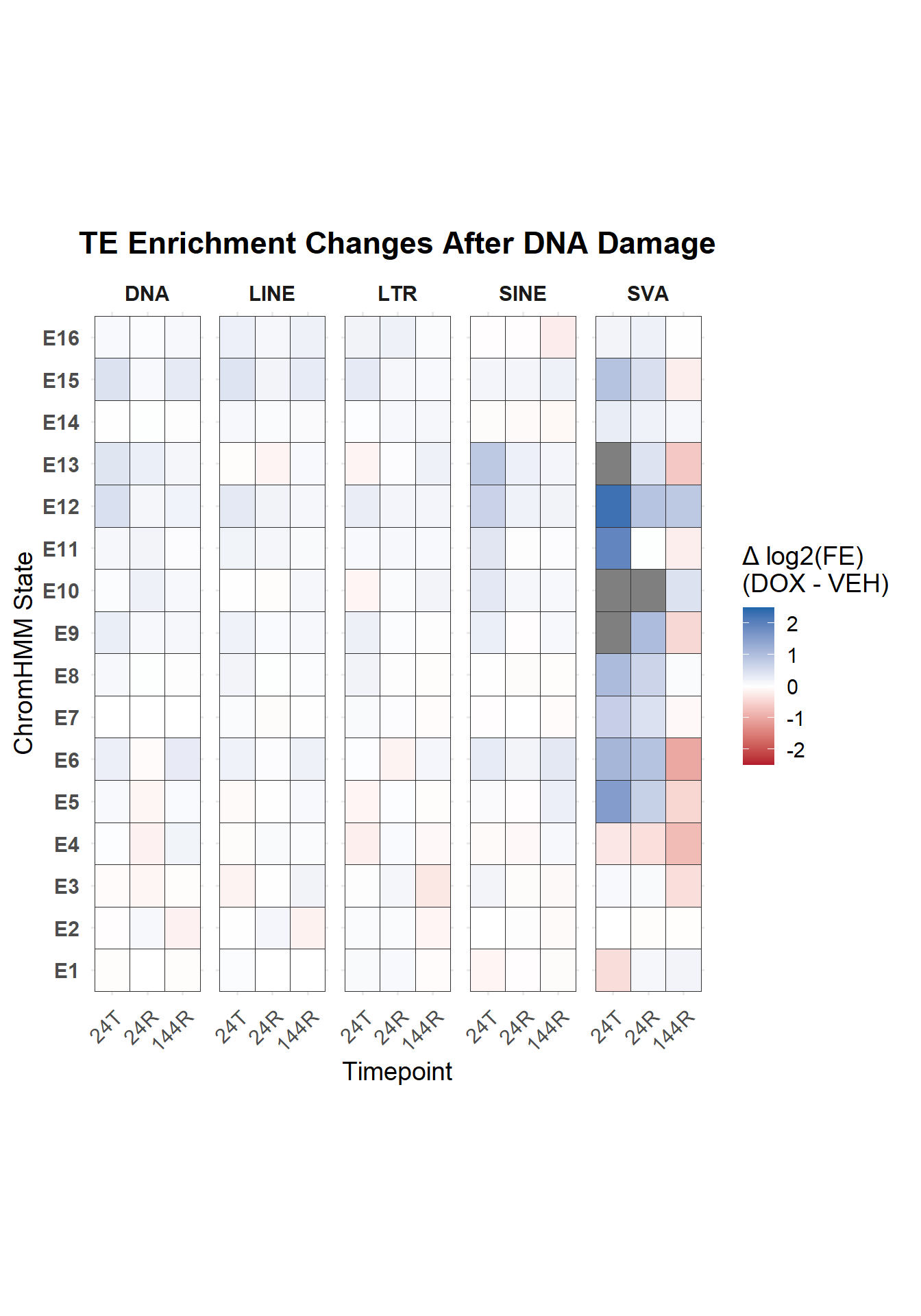
TE_delta_df <- delta_TE_df %>%
  filter(rpt %in% c("LTR","LINE","SINE","DNA","SVA")) %>%
  mutate(
    `State (Emission order)` = forcats::fct_rev(`State (Emission order)`),
    time = factor(time, levels = c("24T","24R","144R"))
  ) %>%
  group_by(rpt) %>%
  mutate(
    # scale relative to max abs value per TE
    delta_log2FE_scaled = delta_log2FE / max(abs(delta_log2FE), na.rm = TRUE),
    # ensure no value goes outside -1..1
    delta_log2FE_scaled = pmax(pmin(delta_log2FE_scaled, 1), -1)
  ) %>%
  ungroup()
# Scale across the entire dataset
# max_abs_delta <- max(abs(TE_delta_df$delta_log2FE_scaled), na.rm = TRUE)

# TE_delta_df <- TE_delta_df %>%
#   mutate(delta_log2FE_scaled = delta_log2FE / max_abs_delta)

ggplot(TE_delta_df,
       aes(x = time,
           y = `State (Emission order)`,
           fill = delta_log2FE_scaled)) +
  geom_tile(color = "grey20", linewidth = 0.2) +

  scale_fill_gradient2(
  low = "#B2182B",
  mid = "white",
  high = "#2166AC",
  midpoint = 0,
  name = "Δ log2(FE)\nscaled"
)+

  facet_wrap(~rpt, ncol = 5) +  # one TE type per facet
  theme_minimal(base_size = 14) +
  theme(
    axis.text.x = element_text(angle = 45, hjust = 1),
    strip.text = element_text(face = "bold"),
    plot.title = element_text(face = "bold", hjust = 0.5)
  ) +
  labs(
    x = "Timepoint",
    y = "ChromHMM State",
    title = "Scaled Δ log2(FE) per TE type after DNA damage"
  ) +
  coord_fixed(ratio = 1.2)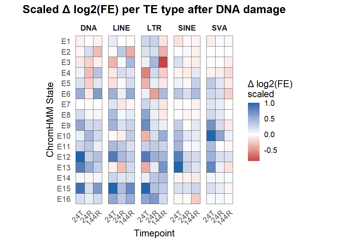
ATAC and cardiac enhancer enrichment
ATAC_long_file <- all_ATAC_states %>%
  filter(`State (Emission order)` != "Base") %>%
  pivot_longer(., -c(`State (Emission order)`,group), names_to = "Identity", values_to="Fold_enrichment") %>%
   mutate(group=factor(group,levels=c("VEH_24T","VEH_24R","VEH_144R","DOX_24T", "DOX_24R", "DOX_144R")),
          `State (Emission order)`=factor(`State (Emission order)`, levels = paste0("E",1:16)))


ATAC_long_file %>%
  # dplyr::filter(stringr::str_detect(Identity, "SCREEN")) %>%
   group_by(Identity) %>%   # i.e. per annotation column
  mutate(
    FE_min = min(Fold_enrichment, na.rm = TRUE),
    FE_max = max(Fold_enrichment, na.rm = TRUE),
    chromhmm_scaled = (Fold_enrichment - FE_min) / (FE_max - FE_min)
  ) %>%
    ggplot(.,aes(x=Identity,y=`State (Emission order)`, fill=chromhmm_scaled))+
  geom_tile(color = "grey9",
            lwd = .1,
            linetype = 1)+
     scale_fill_gradient(
  low = "white",
  high = "#08306B",
  limits = c(0, 1),   # <- KEY
  oob = scales::squish,
   na.value = "white",   # <- this sets NAs to white
  name = "transformed scale"
)+
  theme(axis.text.x = element_text(angle = 45, hjust = 1))+
  facet_wrap(~group, nrow=1, ncol=6)+
    scale_y_discrete(limits=rev)+
  ggtitle("CAR/DAR and cardiac Enhancer types enrichment across states")+
  coord_fixed()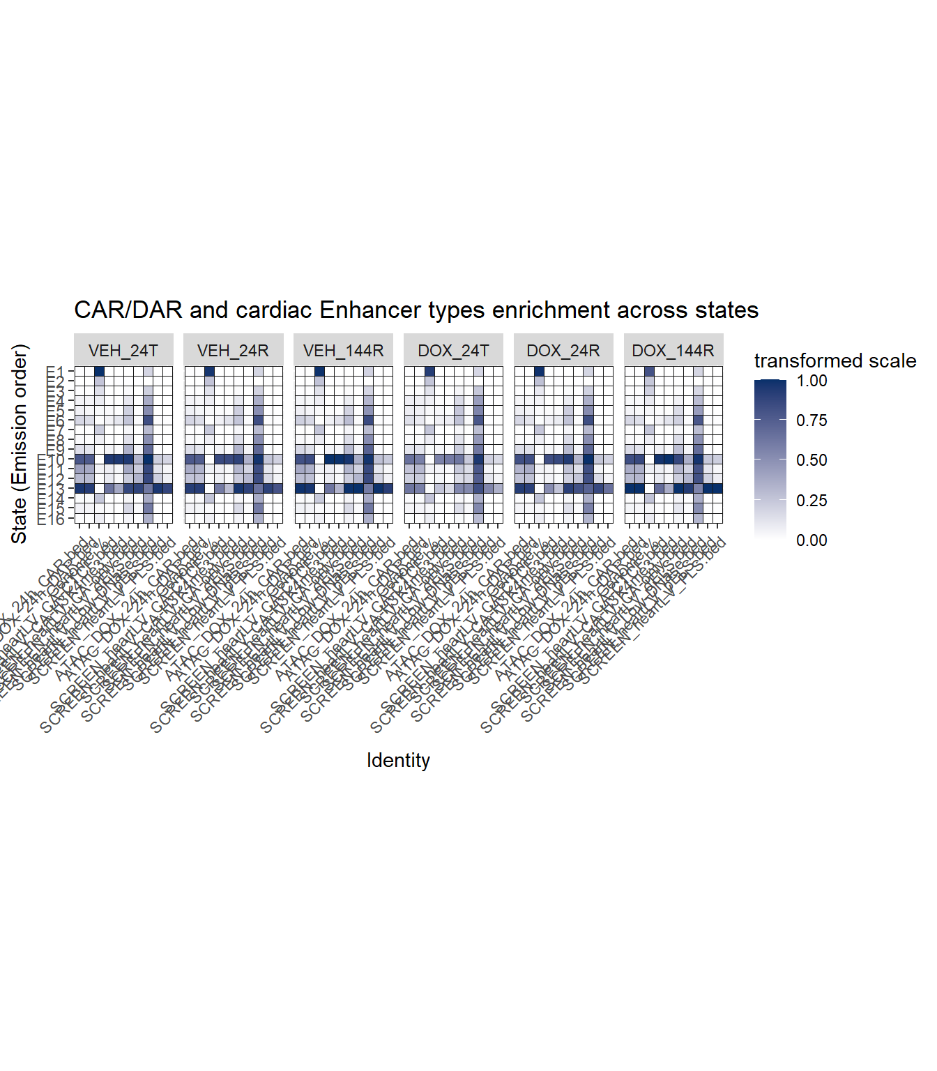
| Version | Author | Date |
|---|---|---|
| 3facb4b | reneeisnowhere | 2026-02-02 |
Looking at SINE elements that overlap H3K27ac ROI elements
SOI data
Now to pull in the segmentation data for just the SOI (states of interest).
##getting all segmentation file locations
seg_files <- list.files(
  "C:/Users/renee/Other_projects_data/DXR_data/TACC_models/Chrom_model_16states_final/",
  pattern = "segments.bed$",
  full.names = TRUE)
### coversion to grages list
chromhmm_gr <- map_df(seg_files, function(f) {
  cond <- basename(f) |> str_remove("_segments.bed")
  import(f) |>
    as.data.frame() |>
    mutate(condition = cond)
})
# saveRDS(chromhmm_gr,"data/RDS_files/chromhmm_granges_segmentation_files.RDS")
autosomes <- paste0("chr", 1:22)
## filtering for the states I want and removing X and y chromosome
chromhmm_sub <- chromhmm_gr %>%
filter(name %in% SOIs) %>%
filter(seqnames %in% autosomes)
repeatmasker <- read_delim("data/Other_paper_data/repeatmasker_20250911.txt",
delim = "\t", escape_double = FALSE,
trim_ws = TRUE)
repeatmasker_clean <- repeatmasker %>% mutate(
strand = ifelse(strand == "C", "-", "+")
) %>%
mutate(
start = genoStart + 1,
end = genoEnd)%>%
mutate(repFamily= str_remove(repFamily, "\\?$")) %>%
# mutate(repClass= str_remove(repClass, "\\?$")) %>%
dplyr::filter(genoName %in% autosomes)
rpt_split <- split(repeatmasker_clean, repeatmasker_clean$repClass)
rpt_split_gr_list <- lapply(rpt_split, function(df) {
GRanges(
seqnames = df$genoName,
ranges = IRanges(start = df$start, end = df$end),
strand = df$strand,
repName = df$repName,
repClass = df$repClass,
repFamily = df$repFamily,
swScore = df$swScore,
milliDiv = df$milliDiv,
id = df$id
)
})
SINE_gr <- rpt_split_gr_list$SINE
LINE_gr <- rpt_split_gr_list$LINE
LTR_gr <- rpt_split_gr_list$LTR
SVA_gr <- rpt_split_gr_list$Retroposon
DNA_gr <- rpt_split_gr_list$DNA
subsetchromhmm_gr <- GRanges(
seqnames = chromhmm_sub$seqnames,
ranges = IRanges(chromhmm_sub$start, chromhmm_sub$end),
state = chromhmm_sub$name,
condition = chromhmm_sub$condition)Questions and overlapping section
H3K27ac_anno_ROIs <- readRDS("data/motif_lists/H3K27ac_annotated_peaks.RDS")

H3K27ac_anno_ROIs_gr <- do.call(c,
  lapply(names(H3K27ac_anno_ROIs), function(group_name) {

    cs <- H3K27ac_anno_ROIs[[group_name]]
    gr <- cs@anno

    # add metadata
    mcols(gr)$set  <- group_name
    mcols(gr)$name <- mcols(gr)$Peakid

    gr}))
seqlevelsStyle(H3K27ac_anno_ROIs_gr)
seqlevelsStyle(subsetchromhmm_gr)

##confirm both use UCSC
H3K27ac_hits <- findOverlaps(H3K27ac_anno_ROIs_gr, subsetchromhmm_gr)
H3K27ac_roi_state_annotated <- H3K27ac_anno_ROIs_gr[queryHits(H3K27ac_hits)]
mcols(H3K27ac_roi_state_annotated) <- cbind(
mcols(H3K27ac_roi_state_annotated),
mcols(subsetchromhmm_gr[subjectHits(H3K27ac_hits)]))
table(mcols(H3K27ac_roi_state_annotated)$state)
table(mcols(H3K27ac_roi_state_annotated)$set, mcols(H3K27ac_roi_state_annotated)$state)
H3K27ac_state_summary <-H3K27ac_roi_state_annotated %>%
as.data.frame() %>%
group_by(set, condition, state) %>%
summarise(
n_peaks = n(),
total_bp = sum(width),
.groups = "drop") %>%
group_by(set, condition) %>%
mutate(
frac_peaks = n_peaks / sum(n_peaks),
frac_bp = total_bp / sum(total_bp)
) %>%
ungroup()### Need to know that an ROI can overlap more than 1 state, say state 11 twice in a set of ROIs.
H3K27ac_roi_state_annotated %>%
as.data.frame() %>%
# distinct(Peakid) ##146222
dplyr::filter(set %in% c("Set_1","Set_2","Set_3")) %>%
# distinct(Peakid) ##114832
dplyr::filter(state=="E10") %>%
# distinct(Peakid)##28,079
group_by(set, condition, Peakid) %>% tally() %>% group_by(n) %>% tally()
### the above show grouping can lead to bp overcounting
H3K27ac_E10_roi_gr <- H3K27ac_roi_state_annotated[ mcols(H3K27ac_roi_state_annotated)$state=="E10" &
mcols(H3K27ac_roi_state_annotated)$set %in% c("Set_1","Set_2","Set_3") ]
# reduce ROIs to merge any duplicates
H3K27ac_E10_roi_gr_unique <- GenomicRanges::reduce(H3K27ac_E10_roi_gr) # merges overlapping ranges within each ROI
# compute bp per set
as.data.frame(H3K27ac_E10_roi_gr_unique)# %>%
group_by(set, condition) %>%
summarise(total_bp = sum(width))
### this just give the exact bp coverage of E10 for bp of ROI in each set and condition.Now I am just going to only pull out unique Peakids by Set and then overlap with repeatmasker data
H3K27ac_E10_roi_df <- H3K27ac_E10_roi_gr %>%
  as.data.frame() %>%
 group_by(Peakid, set, condition, seqnames) %>%
  summarise(
    start = min(start),
    end = max(end),
    .groups = "drop")

H3K27ac_E10_roi_reduced_gr <- GRanges(
  seqnames = H3K27ac_E10_roi_df$seqnames,
  ranges = IRanges(start = H3K27ac_E10_roi_df$start, end = H3K27ac_E10_roi_df$end),
  Peakid = H3K27ac_E10_roi_df$Peakid,
  set = H3K27ac_E10_roi_df$set,
  condition = H3K27ac_E10_roi_df$condition)

te_list <- c("LINE","SINE","LTR","DNA","Retroposon")

H3K27ac_E10_roi_te_hits <- lapply(te_list, function(te_class) {
  te_gr <- rpt_split_gr_list[[te_class]]

  hits <- findOverlaps(H3K27ac_E10_roi_reduced_gr, te_gr)
  if (length(hits) == 0) return(NULL)

  roi_hits <- H3K27ac_E10_roi_reduced_gr[queryHits(hits)]

  mcols(roi_hits)$TE_class <- te_class
  mcols(roi_hits)$repClass <- mcols(te_gr)$repClass[subjectHits(hits)]
  mcols(roi_hits)$repFamily <- mcols(te_gr)$repFamily[subjectHits(hits)]
  mcols(roi_hits)$repName <- mcols(te_gr)$repName[subjectHits(hits)]

  roi_hits
})

names(H3K27ac_E10_roi_te_hits) <- te_list
extract_enrichment <- function(perm_obj, condition_name = NULL) {
# Extract observed overlaps
obs <- perm_obj$numOverlaps$observed
# Extract expected overlaps (mean of permuted)
exp <- mean(perm_obj$numOverlaps$permuted)
# Enrichment ratio
enrich <- obs / exp
# Z-score
zscore <- perm_obj$numOverlaps$zscore
# Return as a data frame
df <- data.frame(
Condition = condition_name,
Observed = obs,
Expected = exp,
Enrichment = enrich,
Zscore = zscore
)
return(df)
}genome_gr <- getGenomeAndMask("hg38")$genome
genome_autosomes <- genome_gr[seqnames(genome_gr) %in% autosomes]
test_set_E10_24T <- H3K27ac_E10_roi_te_hits$LINE[ mcols(H3K27ac_E10_roi_te_hits$LINE)$condition=="24T_DOX_16" &
mcols(H3K27ac_E10_roi_te_hits$LINE)$set == "Set_2" ]
test_set_E10_24R <- H3K27ac_E10_roi_te_hits$LINE[ mcols(H3K27ac_E10_roi_te_hits$LINE)$condition=="24R_DOX_16" &
mcols(H3K27ac_E10_roi_te_hits$LINE)$set == "Set_2" ]
test_set_E10_144R <- H3K27ac_E10_roi_te_hits$LINE[ mcols(H3K27ac_E10_roi_te_hits$LINE)$condition=="144R_DOX_16" &
mcols(H3K27ac_E10_roi_te_hits$LINE)$set == "Set_2" ]
#
perm_test_24T_E10_s2_H3K27ac <- permTest(A= test_set_E10_24T,
B= rpt_split_gr_list$LINE,
ntimes=1000,
randomize.function=randomizeRegions,
evaluate.function = numOverlaps,
genome=genome_autosomes,
count.once= TRUE,
verbose = TRUE)
perm_test_24R_E10_s2_H3K27ac <- permTest(A= test_set_E10_24R,
B= rpt_split_gr_list$LINE,
ntimes=1000,
randomize.function=randomizeRegions,
evaluate.function = numOverlaps,
genome=genome_autosomes,
count.once= TRUE,
verbose = TRUE)
perm_test_144R_E10_s2_H3K27ac <- permTest(A= test_set_E10_144R,
B= rpt_split_gr_list$LINE,
ntimes=1000,
randomize.function=randomizeRegions,
evaluate.function = numOverlaps,
genome=genome_autosomes,
count.once= TRUE,
verbose = TRUE)
#
# A <- extract_enrichment(perm_test_24T_E10_s2_H3K27ac,"S2_E10_24T" )
# B <- extract_enrichment(perm_test_24R_E10_s2_H3K27ac,"S2_E10_24R" )
# C <- extract_enrichment(perm_test_144R_E10_s2_H3K27ac,"S2_E10_144R" )
# test <- bind_rows(A,B,C)
plot(perm_test_24R_E10_s2_H3K27ac)
plot(perm_test_24T_E10_s2_H3K27ac)
plot(perm_test_144R_E10_s2_H3K27ac)
# saveRDS(test, "data/RDS_files/permtest_H3K27ac_S2_LINE.RDS")H3K27ac_144R_set1_summary <- H3K27ac_state_summary %>%
filter(set == "Set_1", condition %in% c("144R_VEH_16", "144R_DOX_16"))
ggplot(H3K27ac_144R_set1_summary, aes(x = condition, y = frac_peaks, fill = state)) +
geom_col(position = "stack") +
ylab("Fraction of peaks per state") +
xlab("Condition") +
scale_fill_brewer(palette = "Set2") +
theme_classic() +
ggtitle("State composition in Set1: VEH144R vs DOX144R")
H3K27ac_144R_set1_wide <- H3K27ac_144R_set1_summary %>%
select(condition, state, frac_peaks) %>%
tidyr::pivot_wider(names_from = condition, values_from = frac_peaks)
H3K27ac_144R_set1_wide <- H3K27ac_144R_set1_wide %>%
mutate(frac_ratio = `144R_DOX_16` / `144R_VEH_16`)
######-24R------------------------------------------------------
H3K27ac_24R_set1_summary <- H3K27ac_state_summary %>%
filter(set == "Set_1", condition %in% c("24R_VEH_16", "24R_DOX_16"))
ggplot(H3K27ac_24R_set1_summary, aes(x = condition, y = frac_peaks, fill = state)) +
geom_col(position = "stack") +
ylab("Fraction of peaks per state") +
xlab("Condition") +
scale_fill_brewer(palette = "Set2") +
theme_classic() +
ggtitle("State composition in Set1: VEH24R vs DOX24R")
H3K27ac_24R_set1_wide <- H3K27ac_24R_set1_summary %>%
select(condition, state, frac_peaks) %>%
tidyr::pivot_wider(names_from = condition, values_from = frac_peaks)
H3K27ac_24R_set1_wide <- H3K27ac_24R_set1_wide %>%
mutate(frac_ratio = `24R_DOX_16` / `24R_VEH_16`)
######-24TR------------------------------------------------------
H3K27ac_24T_set1_summary <- H3K27ac_state_summary %>%
filter(set == "Set_1", condition %in% c("24T_VEH_16", "24T_DOX_16"))
ggplot(H3K27ac_24T_set1_summary, aes(x = condition, y = frac_peaks, fill = state)) +
geom_col(position = "stack") +
ylab("Fraction of peaks per state") +
xlab("Condition") +
scale_fill_brewer(palette = "Set2") +
theme_classic() +
ggtitle("State composition in Set1: VEH24T vs DOX24T")
H3K27ac_24T_set1_wide <- H3K27ac_24T_set1_summary %>%
select(condition, state, frac_peaks) %>%
tidyr::pivot_wider(names_from = condition, values_from = frac_peaks)
H3K27ac_24T_set1_wide <- H3K27ac_24T_set1_wide %>%
mutate(frac_ratio = `24T_DOX_16` / `24T_VEH_16`)Graphing what I have so far. I grouped the overlapping data by sets, so I have all ROIs, all set_1 ROIs, all set_2 rois all set_3 rois.
Now I want to see the breakdown of these states across condtitions in my ROIs- note I have already done a Fold enrichment, so this should mimic that.
ggplot(H3K27ac_state_summary, aes(x = set, y = frac_peaks, fill = state)) +
  geom_col(position = "stack") +
  facet_wrap(~condition) +
  ylab("Fraction of peaks per state") +
  xlab("ROI Set") +
  scale_fill_brewer(palette = "Set2") +
  theme_classic()

table1 <- table(
  H3K27ac_roi_state_annotated$set[H3K27ac_roi_state_annotated$condition == "144R_VEH_16"],
  H3K27ac_roi_state_annotated$state[H3K27ac_roi_state_annotated$condition == "144R_VEH_16"]
)

chisq.test(table1)
sessionInfo()R version 4.4.2 (2024-10-31 ucrt)
Platform: x86_64-w64-mingw32/x64
Running under: Windows 11 x64 (build 26200)
Matrix products: default
locale:
[1] LC_COLLATE=English_United States.utf8
[2] LC_CTYPE=English_United States.utf8
[3] LC_MONETARY=English_United States.utf8
[4] LC_NUMERIC=C
[5] LC_TIME=English_United States.utf8
time zone: America/Chicago
tzcode source: internal
attached base packages:
[1] grid stats4 stats graphics grDevices utils datasets
[8] methods base
other attached packages:
[1] regioneR_1.38.0 ChIPseeker_1.42.1 readxl_1.4.5
[4] DT_0.33 ggrepel_0.9.6 rtracklayer_1.66.0
[7] genomation_1.38.0 plyranges_1.26.0 GenomicRanges_1.58.0
[10] GenomeInfoDb_1.42.3 IRanges_2.40.1 S4Vectors_0.44.0
[13] BiocGenerics_0.52.0 lubridate_1.9.4 forcats_1.0.0
[16] stringr_1.5.1 dplyr_1.1.4 purrr_1.1.0
[19] readr_2.1.5 tidyr_1.3.1 tibble_3.3.0
[22] ggplot2_3.5.2 tidyverse_2.0.0 workflowr_1.7.1
loaded via a namespace (and not attached):
[1] RColorBrewer_1.1-3
[2] rstudioapi_0.17.1
[3] jsonlite_2.0.0
[4] magrittr_2.0.3
[5] ggtangle_0.0.7
[6] GenomicFeatures_1.58.0
[7] farver_2.1.2
[8] rmarkdown_2.29
[9] fs_1.6.6
[10] BiocIO_1.16.0
[11] zlibbioc_1.52.0
[12] vctrs_0.6.5
[13] memoise_2.0.1
[14] Rsamtools_2.22.0
[15] RCurl_1.98-1.17
[16] ggtree_3.14.0
[17] htmltools_0.5.8.1
[18] S4Arrays_1.6.0
[19] TxDb.Hsapiens.UCSC.hg19.knownGene_3.2.2
[20] plotrix_3.8-4
[21] curl_7.0.0
[22] cellranger_1.1.0
[23] SparseArray_1.6.2
[24] gridGraphics_0.5-1
[25] sass_0.4.10
[26] KernSmooth_2.23-26
[27] bslib_0.9.0
[28] htmlwidgets_1.6.4
[29] plyr_1.8.9
[30] impute_1.80.0
[31] cachem_1.1.0
[32] GenomicAlignments_1.42.0
[33] igraph_2.1.4
[34] whisker_0.4.1
[35] lifecycle_1.0.4
[36] pkgconfig_2.0.3
[37] Matrix_1.7-3
[38] R6_2.6.1
[39] fastmap_1.2.0
[40] GenomeInfoDbData_1.2.13
[41] MatrixGenerics_1.18.1
[42] enrichplot_1.26.6
[43] digest_0.6.37
[44] aplot_0.2.8
[45] colorspace_2.1-1
[46] patchwork_1.3.2
[47] AnnotationDbi_1.68.0
[48] ps_1.9.1
[49] rprojroot_2.1.1
[50] RSQLite_2.4.3
[51] labeling_0.4.3
[52] timechange_0.3.0
[53] httr_1.4.7
[54] abind_1.4-8
[55] compiler_4.4.2
[56] bit64_4.6.0-1
[57] withr_3.0.2
[58] BiocParallel_1.40.2
[59] DBI_1.2.3
[60] gplots_3.2.0
[61] R.utils_2.13.0
[62] rappdirs_0.3.3
[63] DelayedArray_0.32.0
[64] rjson_0.2.23
[65] caTools_1.18.3
[66] gtools_3.9.5
[67] tools_4.4.2
[68] ape_5.8-1
[69] httpuv_1.6.16
[70] R.oo_1.27.1
[71] glue_1.8.0
[72] restfulr_0.0.16
[73] callr_3.7.6
[74] nlme_3.1-168
[75] GOSemSim_2.32.0
[76] promises_1.3.3
[77] getPass_0.2-4
[78] gridBase_0.4-7
[79] reshape2_1.4.4
[80] fgsea_1.32.4
[81] generics_0.1.4
[82] gtable_0.3.6
[83] BSgenome_1.74.0
[84] tzdb_0.5.0
[85] R.methodsS3_1.8.2
[86] seqPattern_1.38.0
[87] data.table_1.17.8
[88] hms_1.1.3
[89] utf8_1.2.6
[90] XVector_0.46.0
[91] pillar_1.11.0
[92] vroom_1.6.5
[93] yulab.utils_0.2.1
[94] later_1.4.2
[95] splines_4.4.2
[96] treeio_1.30.0
[97] lattice_0.22-7
[98] bit_4.6.0
[99] tidyselect_1.2.1
[100] GO.db_3.20.0
[101] Biostrings_2.74.1
[102] knitr_1.50
[103] git2r_0.36.2
[104] SummarizedExperiment_1.36.0
[105] xfun_0.52
[106] Biobase_2.66.0
[107] matrixStats_1.5.0
[108] stringi_1.8.7
[109] UCSC.utils_1.2.0
[110] lazyeval_0.2.2
[111] boot_1.3-32
[112] ggfun_0.2.0
[113] yaml_2.3.10
[114] evaluate_1.0.5
[115] codetools_0.2-20
[116] qvalue_2.38.0
[117] ggplotify_0.1.2
[118] cli_3.6.5
[119] processx_3.8.6
[120] jquerylib_0.1.4
[121] dichromat_2.0-0.1
[122] Rcpp_1.1.0
[123] png_0.1-8
[124] XML_3.99-0.18
[125] parallel_4.4.2
[126] blob_1.2.4
[127] DOSE_4.0.1
[128] bitops_1.0-9
[129] tidytree_0.4.6
[130] scales_1.4.0
[131] crayon_1.5.3
[132] rlang_1.1.6
[133] fastmatch_1.1-6
[134] cowplot_1.2.0
[135] KEGGREST_1.46.0