Design Notes
Ross Gayler
2021-06-17
Last updated: 2021-06-25
Checks: 7 0
Knit directory:
VSA_altitude_hold/
This reproducible R Markdown analysis was created with workflowr (version 1.6.2). The Checks tab describes the reproducibility checks that were applied when the results were created. The Past versions tab lists the development history.
Great! Since the R Markdown file has been committed to the Git repository, you know the exact version of the code that produced these results.
Great job! The global environment was empty. Objects defined in the global environment can affect the analysis in your R Markdown file in unknown ways. For reproduciblity it’s best to always run the code in an empty environment.
The command set.seed(20210617) was run prior to running the code in the R Markdown file.
Setting a seed ensures that any results that rely on randomness, e.g.
subsampling or permutations, are reproducible.
Great job! Recording the operating system, R version, and package versions is critical for reproducibility.
Nice! There were no cached chunks for this analysis, so you can be confident that you successfully produced the results during this run.
Great job! Using relative paths to the files within your workflowr project makes it easier to run your code on other machines.
Great! You are using Git for version control. Tracking code development and connecting the code version to the results is critical for reproducibility.
The results in this page were generated with repository version fa4e8f9. See the Past versions tab to see a history of the changes made to the R Markdown and HTML files.
Note that you need to be careful to ensure that all relevant files for the
analysis have been committed to Git prior to generating the results (you can
use wflow_publish or wflow_git_commit). workflowr only
checks the R Markdown file, but you know if there are other scripts or data
files that it depends on. Below is the status of the Git repository when the
results were generated:
Ignored files:
    Ignored:    .Rhistory
    Ignored:    .Rproj.user/
    Ignored:    renv/library/
    Ignored:    renv/staging/
Note that any generated files, e.g. HTML, png, CSS, etc., are not included in this status report because it is ok for generated content to have uncommitted changes.
These are the previous versions of the repository in which changes were made
to the R Markdown (analysis/design_notes.Rmd) and HTML (docs/design_notes.html)
files. If you’ve configured a remote Git repository (see
?wflow_git_remote), click on the hyperlinks in the table below to
view the files as they were in that past version.
| File | Version | Author | Date | Message |
|---|---|---|---|---|
| Rmd | d95c186 | Ross Gayler | 2021-06-25 | WIP |
| html | d95c186 | Ross Gayler | 2021-06-25 | WIP |
| Rmd | b2960d9 | Ross Gayler | 2021-06-24 | WIP |
| html | b2960d9 | Ross Gayler | 2021-06-24 | WIP |
| Rmd | 5707858 | Ross Gayler | 2021-06-24 | WIP |
| html | 5707858 | Ross Gayler | 2021-06-24 | WIP |
| Rmd | 46be0d6 | Ross Gayler | 2021-06-22 | WIP |
| html | 46be0d6 | Ross Gayler | 2021-06-22 | WIP |
| Rmd | 456a363 | Ross Gayler | 2021-06-21 | Add automatic rendering of DFDs |
| html | 456a363 | Ross Gayler | 2021-06-21 | Add automatic rendering of DFDs |
| Rmd | d8b9d53 | Ross Gayler | 2021-06-18 | Add DFD for Design 01 |
| html | d8b9d53 | Ross Gayler | 2021-06-18 | Add DFD for Design 01 |
| Rmd | 0b7e1d4 | Ross Gayler | 2021-06-17 | Publish initial docs |
| html | 0b7e1d4 | Ross Gayler | 2021-06-17 | Publish initial docs |
This notebook records the design considerations behind implementing altitude hold in VSA.
1 Drop-in strategy
Limit the initial problem to altitude hold because this is one-dimensional (as opposed to fully general flight control). This is done to simplify the problem as much as possible.
Treat the VSA components as drop-in replacements for standard control circuitry. This reduces the probability that we will hit an obstacle requiring us to completely reconceptualise how altitude hold is done. On the other hand, it means that we will parallel the classical altitude hold computation, so we may miss seeing some (hypothetical) VSA-centric solution that has no classical analogue.
2 Design issues
2.1 PID controller
The existing classically implemented computation is a PID controller
By my reading there is no claim to the optimality of PID controllers. Rather, they are simple and in widespread use.
My reading also suggests there are plenty of PID variants that are engineering solutions to issues with basic PID.
I conclude there is nothing sacrosanct about PID control, and it is possible that other PID variants or completely different approaches to process control may be more amenable to VSA implementation.
Nonetheless, I will stick with attempting a VSA implementation of the existing PID controller because of the commitment to a drop-in replacement strategy.
The concept of drop-in replacement makes most sense when replacing individual components of the data flow graph.
VSA replacement of larger components of the data flow graph (in the extreme, treating the entire PID controller as a single VSA function) arguably loses the PID structure, because those components no longer exist as separable mechanisms.
2.2 Parameterisation
The classically implemented PID controller has four parameters: \(k_{tgt}\), \(k_p\), \(k_i\), \(k_{windup}\)
\(k_{tgt}\), the target holding altitude, should arguably be a variable rather than a parameter. In the current implementation it is set to the constant value of 5 metres. A more general implementation would allow the hold altitude to be set arbitrarily.
- If this is treated as a variable it will need to be explicitly represented as a VSA value even if the value is held constant during simulations.
- Parameters which are treated as constants do not need to be explicitly represented as VSA values and their effect can be absorbed into the surrounding function (like currying)
The remaining three parameters are for tuning the PID process to minimise overshoot and other undesired behaviours.
There are interactions between the parameters (in terms of their joint effect on the system behaviour).
- For example, \(k_i\) is relatively large in the classically implemented system at least in part to compensate for \(k_{windup}\) being relatively small.
VSA representations of scalar values have a limited range, which must be specified.
Consequently, I have guessed what might be plausible ranges for the parameters if they were to be treated as variables. Don’t takes these ranges too seriously.
The values of some variables in the data flow graph are functions of the parameters, so the ranges of these variables depend in part on the ranges I have guessed for the parameters.
The specific parameterisation of the classically implemented PID controller may not be the most amenable to VSA implementation. For example, the wide value range for some variables caused by the (guessed) wide value range for some parameters may have the effect of making the computation more noisy.
- The parameters \(k_p\) and \(k_i\) effectively control the relativel contribution of the error and integrated error terms to the motor demand. If the error and integrated error variables were scaled to have identical ranges and \(k_p\) scaled to the range \([0, 1]\) then the two terms could be weighted by \(k_p\) and \(1 - k_p\) respectively, which would probably be better for VSA implementation.
2.3 Interfacing
How do we interface between the VSA components and the classical components?
VSA values are very high dimensional vectors.
The values in the classical implementation of the data flow diagram are very low dimensional vectors (typically scalars).
The surrounding machinery of the multicopter simulation assumes that the inputs to and outputs from the altitude hold are classical values. Therefore interfaces are need to convert between the classical and VSA representations.
The interfaces between the classical and VSA are essentially projections between low and high dimensional vector spaces.
2.4 Representation of scalars
Magnitude vs. spatial
Range limits
Noise/resolution
2.5 Temporal issues
Standard VSA is point-in-time/static (some implementations may be inherently temporal)
Embedded in discrete-time simulation. Compatibility of time scales.
Temporal resolution of signals?
Low-pass filters on everything?
2.6 Initialisation
- Classical implementation has explicit initialisation. Do we need special VSA circuits to guarantee orderly turn-on? Could we have an “always-on” VSA design?
3 Design 01 - No VSA
This section deals with the altitude hold controller before the introduction of any VSA components.
3.1 Data Flow Diagram
The data flow diagram represents the desired calculation for altitude hold.
The data flow diagram is derived from
AltitudeHoldPidController.Each node in the diagram represents a potentially inspectable value or the application of a function
Each directed edge in the diagram represents a value flow from one node to another
Think of the data flow diagram as specifying an electronic analog computer where the nodes correspond to function blocks and the edges correspond to wires.
This is the diagram supplied by Simon Levy.
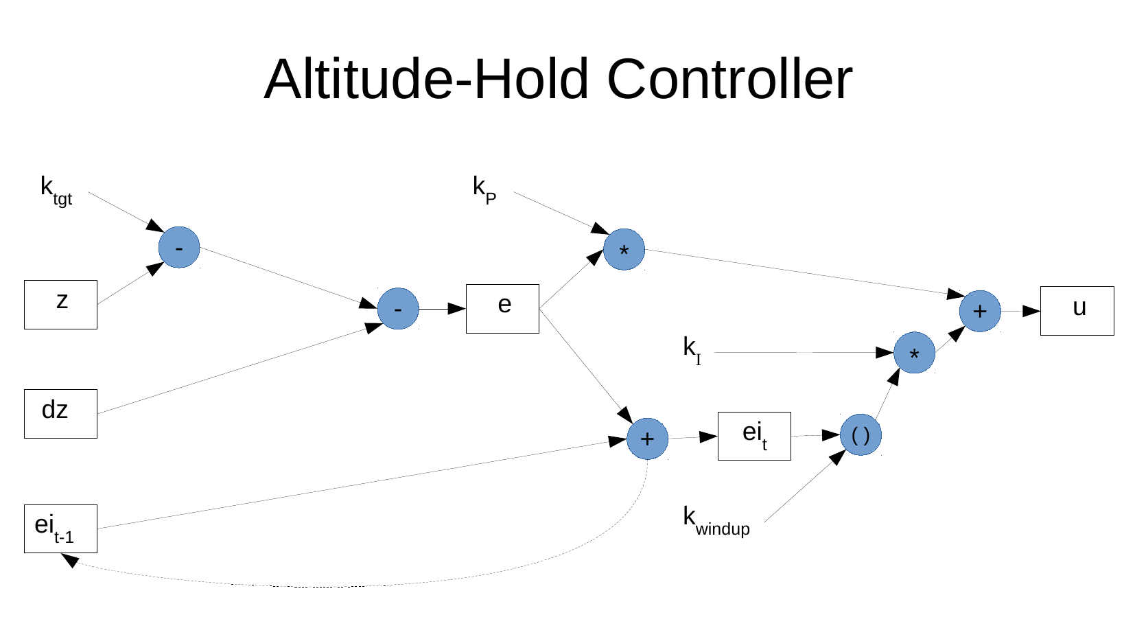
Each node should be interpreted as being implicitly subscripted by time. Only the ei nodes are explicitly subscripted by time.
The value of the u node is constrained to the range [0, 1]. This can be interpreted as implying that there should be an application of a function to constrain the value to that range. This will be inserted in the diagram below.
The integrated error \(ei_t\) is actually implemented as the integration after the clipping by by \(k_{windup}\) is applied. (This is corrected in the following diagram.
This is the diagram reformatted to be consistent with later data flow diagrams.
Parameter nodes are coloured white. These are constant values.
Input nodes are coloured yellow. These are variable values over time.
Output nodes are coloured orange. These are variable values over time.
Internal value nodes are coloured light blue. These are variable values over time.
Function nodes are coloured deep sky blue (the darker shade of blue). These are variable values over time.
All functions except subtraction are commutative, so the mapping from input edges to function arguments is irrelevant.
Because the subtraction function is non-commutative, the two input edges must be mapped to the correct function arguments. The edges are labelled “+” (first argument) and “-” (second argument).
This data flow diagram represents the classically implemented computation, so each value is a scalar real.
Each node is labelled so that they can be referred to.
- The function nodes are labelled with the function name, then a unique label in parentheses.
Each node should be interpreted as being implicitly subscripted by time.
3.2 Data flow tables
The data flow diagram is specified in an external spreadsheet. This allows extra attributes to be associated with the nodes and edges and provides a tolerable user interface for editing the specifications. These tables record more detail about the data flow diagram than can be reasonably displayed on the data flow graph.
For each value (node) , what is it’s range? A physical implementation necessarily has limits. This may render \(k_{windup}\) and
constrainredundant.I have guessed values for the ranges of the variables (informed by the analysis of the simulation data).
_ The ranges for the parameters are truly plucked from the air.
For each value (node) , what is it’s value resolution? This is equivalent asking the noise level that can be tolerated.
For each value (node) , what is it’s temporal resolution? This is equivalent how rapidly we expect the value to change. Some nodes are constant parameters. For time-varying signals do we expect them to alternate between the extreme values on successive samples?
A related point: this is a discrete-time simulation - is the time step fixed? What is the time step? The simplest VSA approach is point-in-time. However, it may be possible to dream up some VSA representation that is essentially temporal, in which case it needs to be compatible with the time-scales of the implementation.
Are there better descriptions for the internal nodes? Something with intuitive meaning of their function would be good.
Does the integrated error needs to be initialised to zero? Does this imply the need for “turn-on” circuitry? Would it be better to have an “always-on” design? Should there be some error correction for cumulative errors?
4 Design 02 - No VSA (tidied)
This is the previous design modified to be more compatible with the VSA changes which will be introduced later.
5 Extreme designs
Digress briefly to consider the extremes of where we might go with incoirporating VSA components into the design of the altitude hold circuit.
5.1 Minimal collapse
Replace all the edges in the data flow diagram with VSA equivalents.
Leave all the vertices in classical form.
The edges are equivalent to wires. A value is inserted at one end and retrieved at the other end. This would require a classical to VSA interface at the input of the edge and a VSA to classical interface at the output end.
This would seem to be an almost pointless thing to do. However, the classical values are assumed to absolutely accurate as mathematical idealisations. Different physical realisations will be inaccurate to some extent. A software implementation would likely represent the values as double-precision floating-point. A very constrained computer might represent the values with 8-bit integers. An analog computer might represent the values as voltages in some constrained range and with noise present in the signal.
Analogously, there can be range, distortion, and noise effects present in VSA representations. There can also be implementation noise, for example if VSA representations are implemented with simulated spiking neurons.
- The minimal collapse scenario would be useful for investigating the effects of VSA representation inaccuracy on the behaviour of the otherwise unaltered altitude hold circuit. This could indicate which values require high fidelity representations.
5.2 Maximal collapse
- Replace the entire set of vertices of the data flow diagram (with the exception of external sources and sinks) with a single vertex. That is, altitude hold is treated as a single, complicated function with no discernible internal data flows. For example, it might be possible to implement the altitude hold as effectively an interpolating lookup table.
Such a model might have advantages depending on the implementation technology.
6 Design 03 -
7 Design 04 -
8 Etc.
R version 4.1.0 (2021-05-18)
Platform: x86_64-pc-linux-gnu (64-bit)
Running under: Ubuntu 21.04

Matrix products: default
BLAS:   /usr/lib/x86_64-linux-gnu/blas/libblas.so.3.9.0
LAPACK: /usr/lib/x86_64-linux-gnu/lapack/liblapack.so.3.9.0

locale:
 [1] LC_CTYPE=en_AU.UTF-8       LC_NUMERIC=C
 [3] LC_TIME=en_AU.UTF-8        LC_COLLATE=en_AU.UTF-8
 [5] LC_MONETARY=en_AU.UTF-8    LC_MESSAGES=en_AU.UTF-8
 [7] LC_PAPER=en_AU.UTF-8       LC_NAME=C
 [9] LC_ADDRESS=C               LC_TELEPHONE=C
[11] LC_MEASUREMENT=en_AU.UTF-8 LC_IDENTIFICATION=C

attached base packages:
[1] stats     graphics  grDevices datasets  utils     methods   base

other attached packages:
[1] DT_0.18            dplyr_1.0.7        DiagrammeR_1.0.6.1 readxl_1.3.1
[5] here_1.0.1

loaded via a namespace (and not attached):
 [1] Rcpp_1.0.6         pillar_1.6.1       compiler_4.1.0     cellranger_1.1.0
 [5] later_1.2.0        RColorBrewer_1.1-2 git2r_0.28.0       workflowr_1.6.2
 [9] tools_4.1.0        digest_0.6.27      jsonlite_1.7.2     evaluate_0.14
[13] lifecycle_1.0.0    tibble_3.1.2       pkgconfig_2.0.3    rlang_0.4.11
[17] rstudioapi_0.13    crosstalk_1.1.1    yaml_2.2.1         xfun_0.24
[21] stringr_1.4.0      knitr_1.33         generics_0.1.0     fs_1.5.0
[25] vctrs_0.3.8        htmlwidgets_1.5.3  tidyselect_1.1.1   rprojroot_2.0.2
[29] glue_1.4.2         R6_2.5.0           fansi_0.5.0        rmarkdown_2.9
[33] bookdown_0.22      tidyr_1.1.3        purrr_0.3.4        magrittr_2.0.1
[37] whisker_0.4        promises_1.2.0.1   ellipsis_0.3.2     htmltools_0.5.1.1
[41] renv_0.13.2        httpuv_1.6.1       utf8_1.2.1         stringi_1.6.2
[45] visNetwork_2.0.9   crayon_1.4.1