Node summary
Robert Schlegel
2019-07-09
Last updated: 2019-08-15
workflowr checks: (Click a bullet for more information)-
✔ R Markdown file: up-to-date
Great! Since the R Markdown file has been committed to the Git repository, you know the exact version of the code that produced these results.
-
✔ Environment: empty
Great job! The global environment was empty. Objects defined in the global environment can affect the analysis in your R Markdown file in unknown ways. For reproduciblity it’s best to always run the code in an empty environment.
-
✔ Seed:
set.seed(20190513)The command
set.seed(20190513)was run prior to running the code in the R Markdown file. Setting a seed ensures that any results that rely on randomness, e.g. subsampling or permutations, are reproducible. -
✔ Session information: recorded
Great job! Recording the operating system, R version, and package versions is critical for reproducibility.
-
Great! You are using Git for version control. Tracking code development and connecting the code version to the results is critical for reproducibility. The version displayed above was the version of the Git repository at the time these results were generated.✔ Repository version: 78f4977
Note that you need to be careful to ensure that all relevant files for the analysis have been committed to Git prior to generating the results (you can usewflow_publishorwflow_git_commit). workflowr only checks the R Markdown file, but you know if there are other scripts or data files that it depends on. Below is the status of the Git repository when the results were generated:
Note that any generated files, e.g. HTML, png, CSS, etc., are not included in this status report because it is ok for generated content to have uncommitted changes.Ignored files: Ignored: .Rhistory Ignored: .Rproj.user/ Ignored: data/ALL_anom.Rda Ignored: data/ALL_clim.Rda Ignored: data/ERA5_lhf.Rda Ignored: data/ERA5_lwr.Rda Ignored: data/ERA5_qnet.Rda Ignored: data/ERA5_qnet_anom.Rda Ignored: data/ERA5_qnet_clim.Rda Ignored: data/ERA5_shf.Rda Ignored: data/ERA5_swr.Rda Ignored: data/ERA5_t2m.Rda Ignored: data/ERA5_t2m_anom.Rda Ignored: data/ERA5_t2m_clim.Rda Ignored: data/ERA5_u.Rda Ignored: data/ERA5_u_anom.Rda Ignored: data/ERA5_u_clim.Rda Ignored: data/ERA5_v.Rda Ignored: data/ERA5_v_anom.Rda Ignored: data/ERA5_v_clim.Rda Ignored: data/GLORYS_mld.Rda Ignored: data/GLORYS_mld_anom.Rda Ignored: data/GLORYS_mld_clim.Rda Ignored: data/GLORYS_u.Rda Ignored: data/GLORYS_u_anom.Rda Ignored: data/GLORYS_u_clim.Rda Ignored: data/GLORYS_v.Rda Ignored: data/GLORYS_v_anom.Rda Ignored: data/GLORYS_v_clim.Rda Ignored: data/NAPA_clim_U.Rda Ignored: data/NAPA_clim_V.Rda Ignored: data/NAPA_clim_W.Rda Ignored: data/NAPA_clim_emp_ice.Rda Ignored: data/NAPA_clim_emp_oce.Rda Ignored: data/NAPA_clim_fmmflx.Rda Ignored: data/NAPA_clim_mldkz5.Rda Ignored: data/NAPA_clim_mldr10_1.Rda Ignored: data/NAPA_clim_qemp_oce.Rda Ignored: data/NAPA_clim_qla_oce.Rda Ignored: data/NAPA_clim_qns.Rda Ignored: data/NAPA_clim_qsb_oce.Rda Ignored: data/NAPA_clim_qt.Rda Ignored: data/NAPA_clim_runoffs.Rda Ignored: data/NAPA_clim_ssh.Rda Ignored: data/NAPA_clim_sss.Rda Ignored: data/NAPA_clim_sst.Rda Ignored: data/NAPA_clim_taum.Rda Ignored: data/NAPA_clim_vars.Rda Ignored: data/NAPA_clim_vecs.Rda Ignored: data/OAFlux.Rda Ignored: data/OISST_sst.Rda Ignored: data/OISST_sst_anom.Rda Ignored: data/OISST_sst_clim.Rda Ignored: data/node_mean_all_anom.Rda Ignored: data/packet_all.Rda Ignored: data/packet_all_anom.Rda Ignored: data/packet_nolab.Rda Ignored: data/packet_nolab14.Rda Ignored: data/packet_nolabgsl.Rda Ignored: data/packet_nolabmod.Rda Ignored: data/som_all.Rda Ignored: data/som_all_anom.Rda Ignored: data/som_nolab.Rda Ignored: data/som_nolab14.Rda Ignored: data/som_nolab_16.Rda Ignored: data/som_nolab_9.Rda Ignored: data/som_nolabgsl.Rda Ignored: data/som_nolabmod.Rda Ignored: data/synoptic_states.Rda Ignored: data/synoptic_vec_states.Rda Untracked files: Untracked: output/SOM/no_ls/assets Untracked: output/SOM/no_ls/no_ls Unstaged changes: Modified: code/functions.R Modified: docs/assets/no_ls/fig_2.pdf Modified: docs/assets/no_ls/fig_3.pdf Modified: docs/assets/no_ls/fig_4.pdf Modified: docs/assets/no_ls/fig_5.pdf Modified: docs/assets/no_ls/fig_6.pdf Modified: docs/assets/no_ls/fig_7.pdf Modified: docs/assets/no_ls/node_10_panels.pdf Modified: docs/assets/no_ls/node_11_panels.pdf Modified: docs/assets/no_ls/node_12_panels.pdf Modified: docs/assets/no_ls/node_1_panels.pdf Modified: docs/assets/no_ls/node_2_panels.pdf Modified: docs/assets/no_ls/node_3_panels.pdf Modified: docs/assets/no_ls/node_4_panels.pdf Modified: docs/assets/no_ls/node_5_panels.pdf Modified: docs/assets/no_ls/node_6_panels.pdf Modified: docs/assets/no_ls/node_7_panels.pdf Modified: docs/assets/no_ls/node_8_panels.pdf Modified: docs/assets/no_ls/node_9_panels.pdf Modified: docs/assets/no_ls_14/fig_2.pdf Modified: docs/assets/no_ls_14/fig_3.pdf Modified: docs/assets/no_ls_14/fig_4.pdf Modified: docs/assets/no_ls_14/fig_5.pdf Modified: docs/assets/no_ls_14/fig_6.pdf Modified: docs/assets/no_ls_14/fig_7.pdf Modified: docs/assets/no_ls_14/node_1_panels.pdf Modified: docs/assets/no_ls_14/node_2_panels.pdf Modified: docs/assets/no_ls_14/node_3_panels.pdf Modified: docs/assets/no_ls_14/node_4_panels.pdf Modified: docs/assets/no_ls_14/node_5_panels.pdf Modified: docs/assets/no_ls_14/node_6_panels.pdf Modified: docs/assets/no_ls_14/node_7_panels.pdf Modified: docs/assets/no_ls_14/node_8_panels.pdf Modified: docs/assets/no_ls_14/node_9_panels.pdf Modified: docs/assets/no_ls_3x3/fig_2.pdf Modified: docs/assets/no_ls_3x3/fig_3.pdf Modified: docs/assets/no_ls_3x3/fig_4.pdf Modified: docs/assets/no_ls_3x3/fig_5.pdf Modified: docs/assets/no_ls_3x3/fig_6.pdf Modified: docs/assets/no_ls_3x3/fig_7.pdf Modified: docs/assets/no_ls_3x3/node_1_panels.pdf Modified: docs/assets/no_ls_3x3/node_2_panels.pdf Modified: docs/assets/no_ls_3x3/node_3_panels.pdf Modified: docs/assets/no_ls_3x3/node_4_panels.pdf Modified: docs/assets/no_ls_3x3/node_5_panels.pdf Modified: docs/assets/no_ls_3x3/node_6_panels.pdf Modified: docs/assets/no_ls_3x3/node_7_panels.pdf Modified: docs/assets/no_ls_3x3/node_8_panels.pdf Modified: docs/assets/no_ls_3x3/node_9_panels.pdf Modified: output/SOM/all/fig_2.pdf Modified: output/SOM/all/fig_3.pdf Modified: output/SOM/all/fig_4.pdf Modified: output/SOM/all/fig_5.pdf Modified: output/SOM/all/fig_6.pdf Modified: output/SOM/all/fig_7.pdf Modified: output/SOM/all/node_10_panels.pdf Modified: output/SOM/all/node_11_panels.pdf Modified: output/SOM/all/node_12_panels.pdf Modified: output/SOM/all/node_1_panels.pdf Modified: output/SOM/all/node_2_panels.pdf Modified: output/SOM/all/node_3_panels.pdf Modified: output/SOM/all/node_4_panels.pdf Modified: output/SOM/all/node_5_panels.pdf Modified: output/SOM/all/node_6_panels.pdf Modified: output/SOM/all/node_7_panels.pdf Modified: output/SOM/all/node_8_panels.pdf Modified: output/SOM/all/node_9_panels.pdf Modified: output/SOM/no_ls/fig_2.pdf Modified: output/SOM/no_ls/fig_3.pdf Modified: output/SOM/no_ls/fig_4.pdf Modified: output/SOM/no_ls/fig_5.pdf Modified: output/SOM/no_ls/fig_6.pdf Modified: output/SOM/no_ls/fig_7.pdf Modified: output/SOM/no_ls/node_10_panels.pdf Modified: output/SOM/no_ls/node_11_panels.pdf Modified: output/SOM/no_ls/node_12_panels.pdf Modified: output/SOM/no_ls/node_1_panels.pdf Modified: output/SOM/no_ls/node_2_panels.pdf Modified: output/SOM/no_ls/node_3_panels.pdf Modified: output/SOM/no_ls/node_4_panels.pdf Modified: output/SOM/no_ls/node_5_panels.pdf Modified: output/SOM/no_ls/node_6_panels.pdf Modified: output/SOM/no_ls/node_7_panels.pdf Modified: output/SOM/no_ls/node_8_panels.pdf Modified: output/SOM/no_ls/node_9_panels.pdf Modified: output/SOM/no_ls_14/fig_2.pdf Modified: output/SOM/no_ls_14/fig_3.pdf Modified: output/SOM/no_ls_14/fig_4.pdf Modified: output/SOM/no_ls_14/fig_5.pdf Modified: output/SOM/no_ls_14/fig_6.pdf Modified: output/SOM/no_ls_14/fig_7.pdf Modified: output/SOM/no_ls_14/node_1_panels.pdf Modified: output/SOM/no_ls_14/node_2_panels.pdf Modified: output/SOM/no_ls_14/node_3_panels.pdf Modified: output/SOM/no_ls_14/node_4_panels.pdf Modified: output/SOM/no_ls_14/node_5_panels.pdf Modified: output/SOM/no_ls_14/node_6_panels.pdf Modified: output/SOM/no_ls_14/node_7_panels.pdf Modified: output/SOM/no_ls_14/node_8_panels.pdf Modified: output/SOM/no_ls_14/node_9_panels.pdf Modified: output/SOM/no_ls_3x3/fig_2.pdf Modified: output/SOM/no_ls_3x3/fig_3.pdf Modified: output/SOM/no_ls_3x3/fig_4.pdf Modified: output/SOM/no_ls_3x3/fig_5.pdf Modified: output/SOM/no_ls_3x3/fig_6.pdf Modified: output/SOM/no_ls_3x3/fig_7.pdf Modified: output/SOM/no_ls_3x3/node_1_panels.pdf Modified: output/SOM/no_ls_3x3/node_2_panels.pdf Modified: output/SOM/no_ls_3x3/node_3_panels.pdf Modified: output/SOM/no_ls_3x3/node_4_panels.pdf Modified: output/SOM/no_ls_3x3/node_5_panels.pdf Modified: output/SOM/no_ls_3x3/node_6_panels.pdf Modified: output/SOM/no_ls_3x3/node_7_panels.pdf Modified: output/SOM/no_ls_3x3/node_8_panels.pdf Modified: output/SOM/no_ls_3x3/node_9_panels.pdf Modified: output/SOM/no_ls_4x4/fig_2.pdf Modified: output/SOM/no_ls_4x4/fig_3.pdf Modified: output/SOM/no_ls_4x4/fig_4.pdf Modified: output/SOM/no_ls_4x4/fig_5.pdf Modified: output/SOM/no_ls_4x4/fig_6.pdf Modified: output/SOM/no_ls_4x4/fig_7.pdf Modified: output/SOM/no_ls_4x4/node_10_panels.pdf Modified: output/SOM/no_ls_4x4/node_11_panels.pdf Modified: output/SOM/no_ls_4x4/node_12_panels.pdf Modified: output/SOM/no_ls_4x4/node_13_panels.pdf Modified: output/SOM/no_ls_4x4/node_14_panels.pdf Modified: output/SOM/no_ls_4x4/node_15_panels.pdf Modified: output/SOM/no_ls_4x4/node_16_panels.pdf Modified: output/SOM/no_ls_4x4/node_1_panels.pdf Modified: output/SOM/no_ls_4x4/node_2_panels.pdf Modified: output/SOM/no_ls_4x4/node_3_panels.pdf Modified: output/SOM/no_ls_4x4/node_4_panels.pdf Modified: output/SOM/no_ls_4x4/node_5_panels.pdf Modified: output/SOM/no_ls_4x4/node_6_panels.pdf Modified: output/SOM/no_ls_4x4/node_7_panels.pdf Modified: output/SOM/no_ls_4x4/node_8_panels.pdf Modified: output/SOM/no_ls_4x4/node_9_panels.pdf Modified: output/SOM/no_ls_gsl/fig_2.pdf Modified: output/SOM/no_ls_gsl/fig_3.pdf Modified: output/SOM/no_ls_gsl/fig_4.pdf Modified: output/SOM/no_ls_gsl/fig_5.pdf Modified: output/SOM/no_ls_gsl/fig_6.pdf Modified: output/SOM/no_ls_gsl/fig_7.pdf Modified: output/SOM/no_ls_gsl/node_10_panels.pdf Modified: output/SOM/no_ls_gsl/node_11_panels.pdf Modified: output/SOM/no_ls_gsl/node_12_panels.pdf Modified: output/SOM/no_ls_gsl/node_1_panels.pdf Modified: output/SOM/no_ls_gsl/node_2_panels.pdf Modified: output/SOM/no_ls_gsl/node_3_panels.pdf Modified: output/SOM/no_ls_gsl/node_4_panels.pdf Modified: output/SOM/no_ls_gsl/node_5_panels.pdf Modified: output/SOM/no_ls_gsl/node_6_panels.pdf Modified: output/SOM/no_ls_gsl/node_7_panels.pdf Modified: output/SOM/no_ls_gsl/node_8_panels.pdf Modified: output/SOM/no_ls_gsl/node_9_panels.pdf Modified: output/SOM/no_ls_mod/fig_2.pdf Modified: output/SOM/no_ls_mod/fig_3.pdf Modified: output/SOM/no_ls_mod/fig_4.pdf Modified: output/SOM/no_ls_mod/fig_5.pdf Modified: output/SOM/no_ls_mod/fig_6.pdf Modified: output/SOM/no_ls_mod/fig_7.pdf Modified: output/SOM/no_ls_mod/node_1_panels.pdf Modified: output/SOM/no_ls_mod/node_2_panels.pdf Modified: output/SOM/no_ls_mod/node_3_panels.pdf Modified: output/SOM/no_ls_mod/node_4_panels.pdf
Expand here to see past versions:
| File | Version | Author | Date | Message |
|---|---|---|---|---|
| Rmd | 78f4977 | robwschlegel | 2019-08-15 | Re-publish entire site. |
| Rmd | eac68d5 | robwschlegel | 2019-08-15 | Finished the first pass over all of the node results. |
| Rmd | 07fe2a2 | robwschlegel | 2019-08-14 | Nearly through the node summaries for the three SOM experiments |
| Rmd | a61b420 | robwschlegel | 2019-08-13 | Working on SOM write-up |
| html | 20ae166 | robwschlegel | 2019-08-11 | Build site. |
| Rmd | d46e344 | robwschlegel | 2019-08-11 | Re-publish entire site. |
| html | 19bea26 | robwschlegel | 2019-08-11 | Build site. |
| Rmd | b6e2cd9 | robwschlegel | 2019-08-11 | Re-publish entire site. |
| html | 2652a3a | robwschlegel | 2019-08-11 | Build site. |
| Rmd | 75c138c | robwschlegel | 2019-08-11 | Re-publish entire site. |
| Rmd | adc762b | robwschlegel | 2019-08-08 | Re-worked the GLORYS data and propogated update through to SOM analysis figures for all experiments |
| html | f0d2efb | robwschlegel | 2019-08-07 | Build site. |
| Rmd | 9d81722 | robwschlegel | 2019-08-07 | Re-publish entire site. |
| Rmd | ed626bf | robwschlegel | 2019-08-07 | Ran a bunch of figures and had a meeting with Eric. More changes coming to GLORYS data tomorrow before settling on one of the experimental SOMs |
| html | d4ba012 | robwschlegel | 2019-07-09 | Build site. |
| Rmd | c8a5a1a | robwschlegel | 2019-07-09 | Fixing figure display in vignette. |
| Rmd | 3a740c2 | robwschlegel | 2019-07-09 | Creating assets folder for displaying figures created in other vignettes in new vignettes etc. |
| html | 3a740c2 | robwschlegel | 2019-07-09 | Creating assets folder for displaying figures created in other vignettes in new vignettes etc. |
| html | 81e961d | robwschlegel | 2019-07-09 | Build site. |
| Rmd | 497eeb2 | robwschlegel | 2019-07-09 | Re-publish entire site. |
| Rmd | 95a168d | robwschlegel | 2019-07-09 | Frame of node summary vignette worked out |
Introduction
This vignette will show the summary figures for the various SOM experiments. The code used to create these summary figures may be found in code/functions.R and a more detailed overview is given in the Figures vignette. The SOM experiments are given below by name and abbreviation. Within each experiment, the individual nodes are listed below by their number. Use the table of contents on the left of the screen to move quickly between SOM experiments and their nodes of interest as desired.
Visualise SOM results
With the following lines of code we create PDFs for each of the variables for each of the nodes for our different conditions. These PDFs may be seen at output/SOM/*, where * is the code name denoting which SOM experiment was conducted.
Juggling back and forth between the SST anomaly figures with and without the Gulf of St Lawrence it first appears that they are very different, but this is mostly due to the top and bottom rows of nodes being flipped. The actual differences are much more muted and the patterns tend to hold. The patterns appear more crisp in the larger of the two study extents. This is likely because the inclusion of the shallow GSL gives more power to the atmospheric variables to compete with the Gulf Stream. For this reason we are going to proceed with the inclusion of the Gulf of St Lawrence.
Looking at different counts of nodes it appears as though 9 may not be enough. When 12 nodes are used more detail comes through. Going up to 16 nodes appear to be too much as not much more detail comes through while creating the complexity of more node results to sift through. When the moderate events are removed we are left with only 37 events (synoptic states) to feed the SOM. This means we shouldn’t use more than 4 nodes so as not to (be just shy of) at least 10 potential values binned into each node. The four nodes that are output do show the most clear difference in patterns and actually do a surprising job of encapsulating the different potential drivers of MHWs. An ANOSIM test on the nodes show that they are different with a p = 0.046. All of the other results have a ANOSIM of p = 0.001. One issue with screening the events by category is that this part of the ocean experiences many long category I Moderate events that may still be relevant.
So rather than screen by category, I also made a run on the SOM with MHW data with events shorter than 14 days removed. This left us with 103 events to work with, which is a good number to use with a 3x3 grid. The results tell perhaps a clearer story than with the 12 nodes and all MHWs.
Just from going over the node summaries created in this vignette it is too difficult to say conclusively which SOM experiment produces the clearest results. We will need to go over the summary figures in much more detail in order to get a better idea of how well this is working out. Also unresolved in this vignette is the criticism that the methodology used for the creation of the mean synoptic states fed to the SOM is weak to long events coming through as “grey”, meaning they average out to a rather unremarkable state, even though they are likely the most important of all. One proposed fix for this is to create synoptic states using only the peak date of the event, rather than a mean over the range of the event. This should be looked into…
A last point here is that this methodology should also be useful for looking backwards and forwards through time to see what the synoptic states looked like leading up to and just after the event. This information could be more useful than the first wave of results. Before doing this however a singular methodology needs to be pinned down (i.e. which events to screen and how many nodes to use).
See the files in the /output/SOM_nodes/ folder in the GitHub repo for this project. They aren’t all shown here because they take a bit too long to render.
Figure summary key
The summaries for the figures below have a lot of acronyms in them but they are consistently used and I will provide a list of what they are here. Whenever one sees an acronym in lower case letters it is referring to one of the regions of the study area as seen in the following figure.
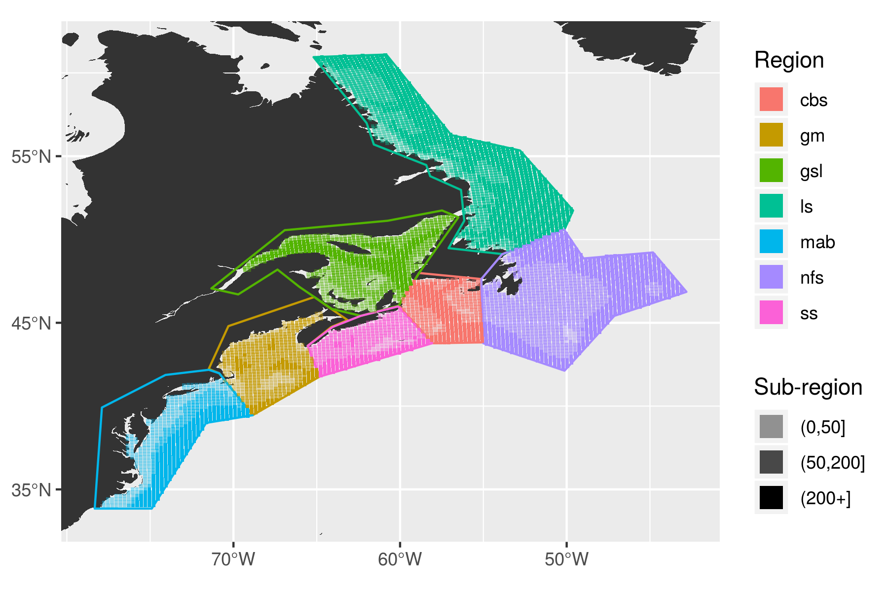
The regions of the coast were devided up by their temperature and salinity regimes based on work by Richaud et al. (2016). The regions were furthered divided into sub-regions based on their depth.
Expand here to see past versions of study_regions.png:
| Version | Author | Date |
|---|---|---|
| 9273f18 | robwschlegel | 2019-08-11 |
The region abbreviations are:
- cbs = Cabot Straight
- gm = Gulf of Maine
- gls = Gulf of St. Lawrence
- ls = Labrador Shelf
- mab = Mid-Atlantic Bight
- nfs = Newfoundland Shelf
- ss = Scotian Shelf
The upper case acronyms used in the following figure captions are as follows:
- SST = Sea surface temperature
- SOM = Self-organising map(s)
- GS = Gulf Stream
- AO = Atlantic Ocean
- LS = Labrador Sea
- LC = Labrador Current
- NS = Nova Scotia
- US = United States
- CN = Canada
It is also worth noting that the scales used to show the variables in the individual node summary figures are not the same across all of the nodes. This was an intentional decision as it allows for more detail to emerge within each node summary. The overall comparisons of nodes are to be done on the figures that show only 2 or 3 variables for all of the nodes at once.
The summary of each individual node has three separate chunks: 1) the MHW metrics, region + season + years of occurrence; 2) the patterns observed in the physical variables; 3) a sentence stating what appears to be the main driver/pattern.
SOM experiment: No Labrador Shelf region (default), 4x3 nodes
There are a total of 289 MHWs considered when putting this 12 node (4x3) SOM together. The largest concentration of MHWs is into the middle two SOM nodes (6 + 7), where there are twice as many events as some of the side and corner nodes. The top left corner, node 1, also has a large amount of events placed within it and the diagonally opposite node (12) has a decent number. Overall I would not have said that any of the nodes have notably fewer events, but further analysis shows that node 8 (middle right) is mostly populated by MHWs from one large event.
Node summary table
The table below contains a concise summary of the nodes following Table 4 in Oliver et al. (2018). The following sub-sections provide more in-depth explanations.
| Node | Region | Season | MHW Properties | Conditions |
|---|---|---|---|---|
| 1 |
Season + region
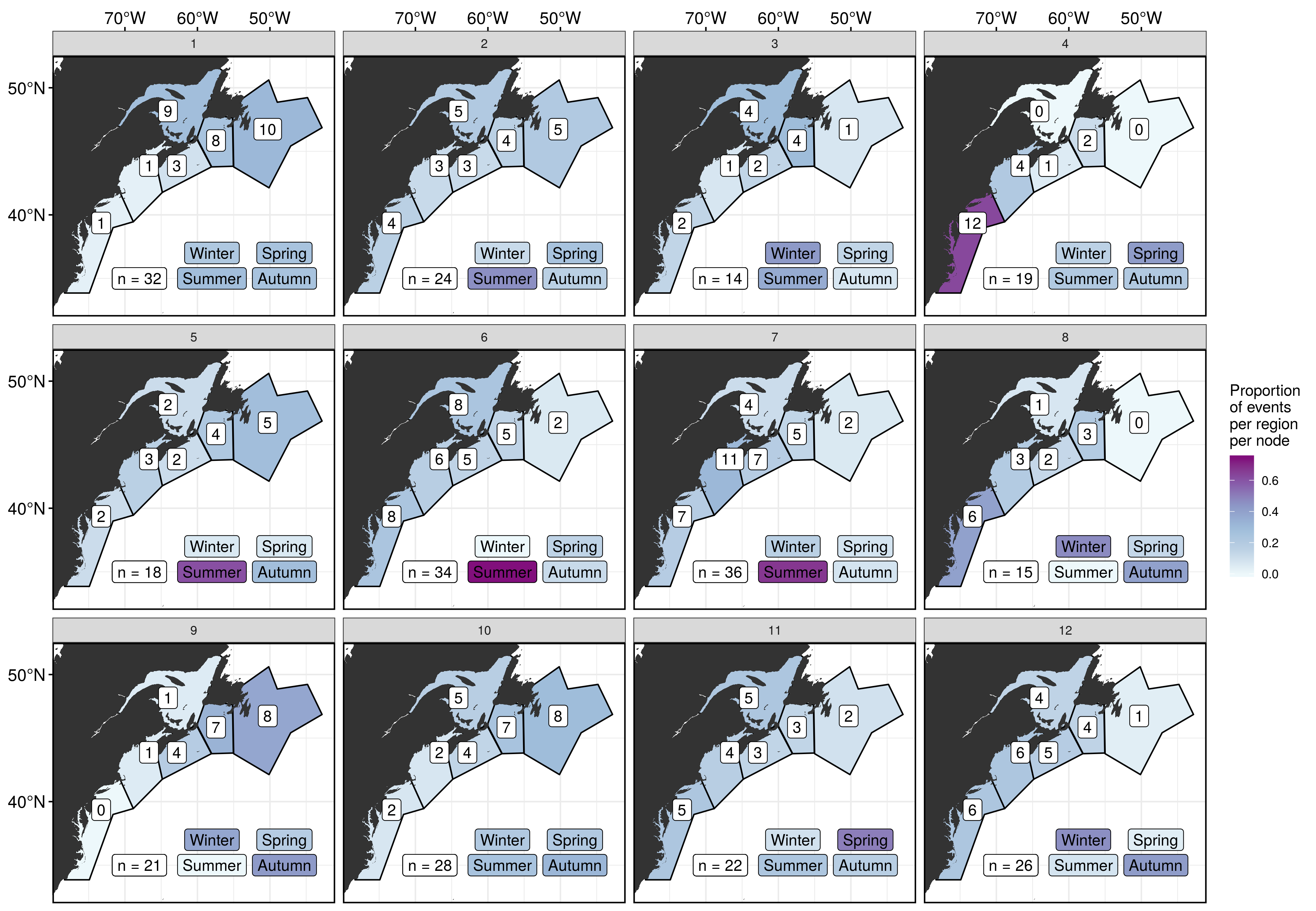
In the figure below we most quickly see that the proportion of MHWs occurring in the middle two nodes are summer events. The seasons are determined by the month during which the peak of the event occurred, with Winter = JFM etc. The nodes on the right-hand have mostly events from the mab. The distribution becomes more even as we move to the centre with the left-hand nodes having mostly nfs and gsl events. The bottom left node has almost no summer events.
Expand here to see past versions of fig_5.png:
| Version | Author | Date |
|---|---|---|
| 9273f18 | robwschlegel | 2019-08-11 |
SST + U + V
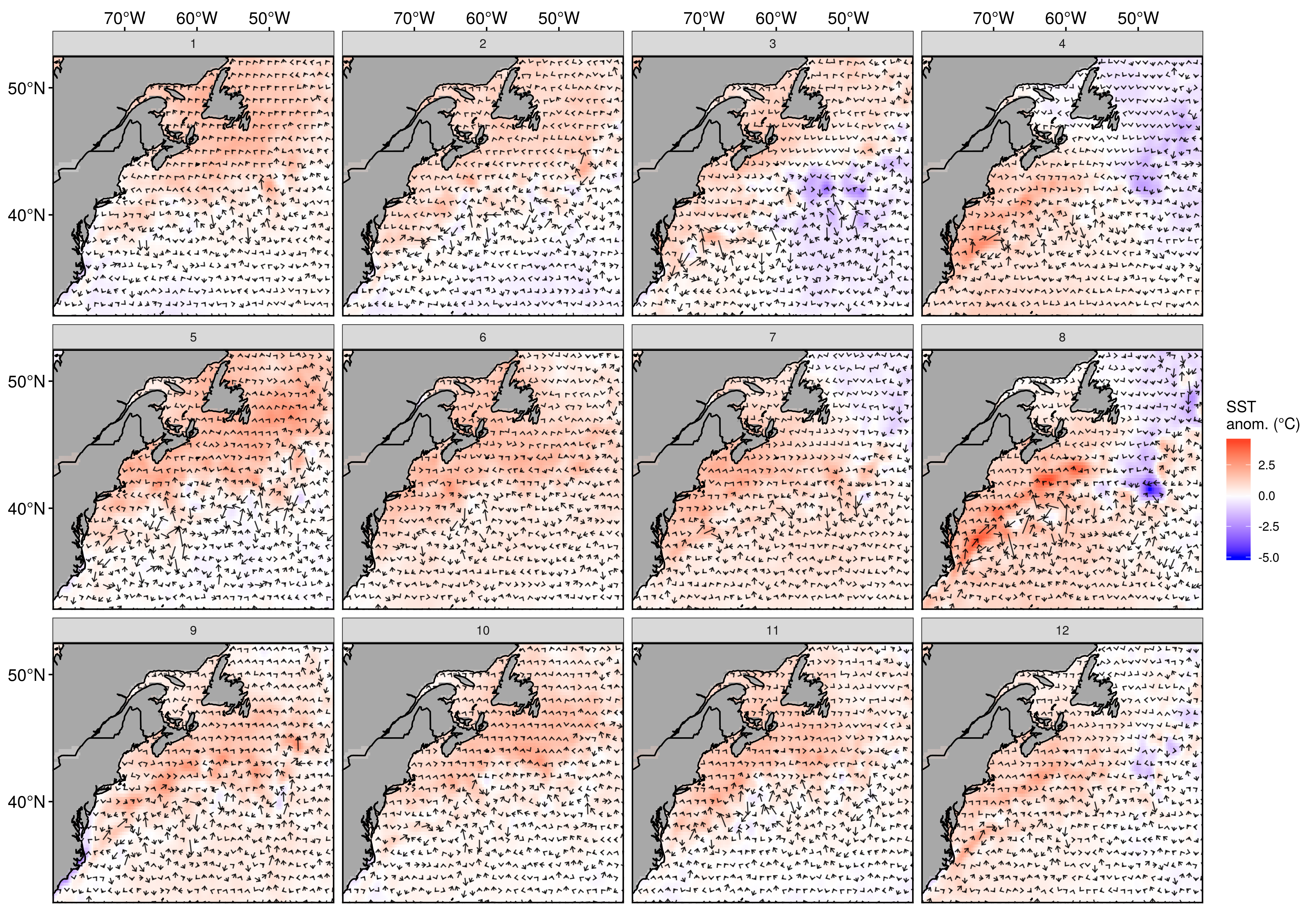
The only U + V anomaly pattern I see is that the centre nodes (6 + 7) and the opposite corners of nodes 1 + 12 show little strength/vorticity in the GS while the other nodes tend to show more. The strength of the GS is apparent in node 8, and the vorticity in the eddy field is very apparent in node 5.
For SST we see moving from the right to the left the LS anomaly tends to go from cool to warm. As we move from the top down the AO tends to become warmer. The gm, gsl, and ss regions are warm in all of the nodes. Most of the SST is anomalously warm in the middle two nodes.
Expand here to see past versions of fig_2.png:
| Version | Author | Date |
|---|---|---|
| 9273f18 | robwschlegel | 2019-08-11 |
Air temp + U + V
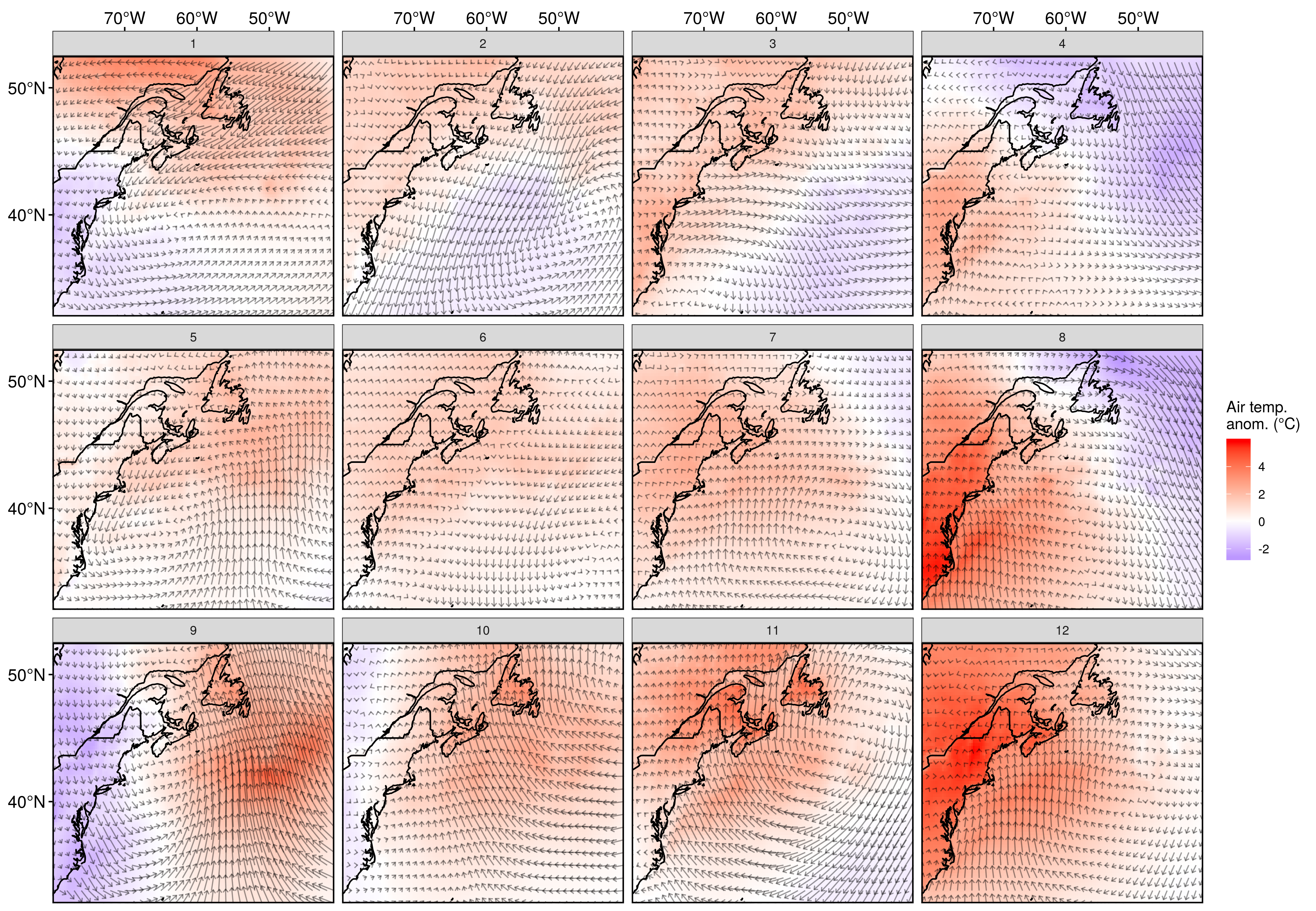
Here we see much clearer patterns.
For air temperature anomalies we see that the air above the LS gets warmer as we move left and down. The air over the USA becomes warmer as we move to the right. Most of the air in the middle two nodes is warm. The air over the AO becomes warmer as we move down the nodes.
One consistent pattern across all of the U + V values is that the top and right-hand sides have strong anomalous wind movement down from the Northeast corner while the bottom right corner nodes have strong northward wind anomalies in their top right corners.
On the right-hand side of the nodes we see generally anti-cyclonic wind movement around a thermal dipole with the southward moving air being anomalously warm. The colder (warmer) th air temperature the faster south (north) the anomalous wind movement is. In the second right-most column (nodes 3 +7 +11) we also see anticyclonic wind anomalies around thermal dipoles. The central position of the anticyclone is different in each node, and the thermal anomalies tend to be less than the right-hand column. Te left-hand two columns have cyclonic wind movement around thermal dipoles with the stronger patterns in the far left column. Node 10 is a bit different in that it appears to have anticyclonic wind movement, but a cold dipole that looks more like the cyclonic movement nodes. The center two nodes have the smaller wind patterns, with node 6 the smallest.
Expand here to see past versions of fig_3.png:
| Version | Author | Date |
|---|---|---|
| 9273f18 | robwschlegel | 2019-08-11 |
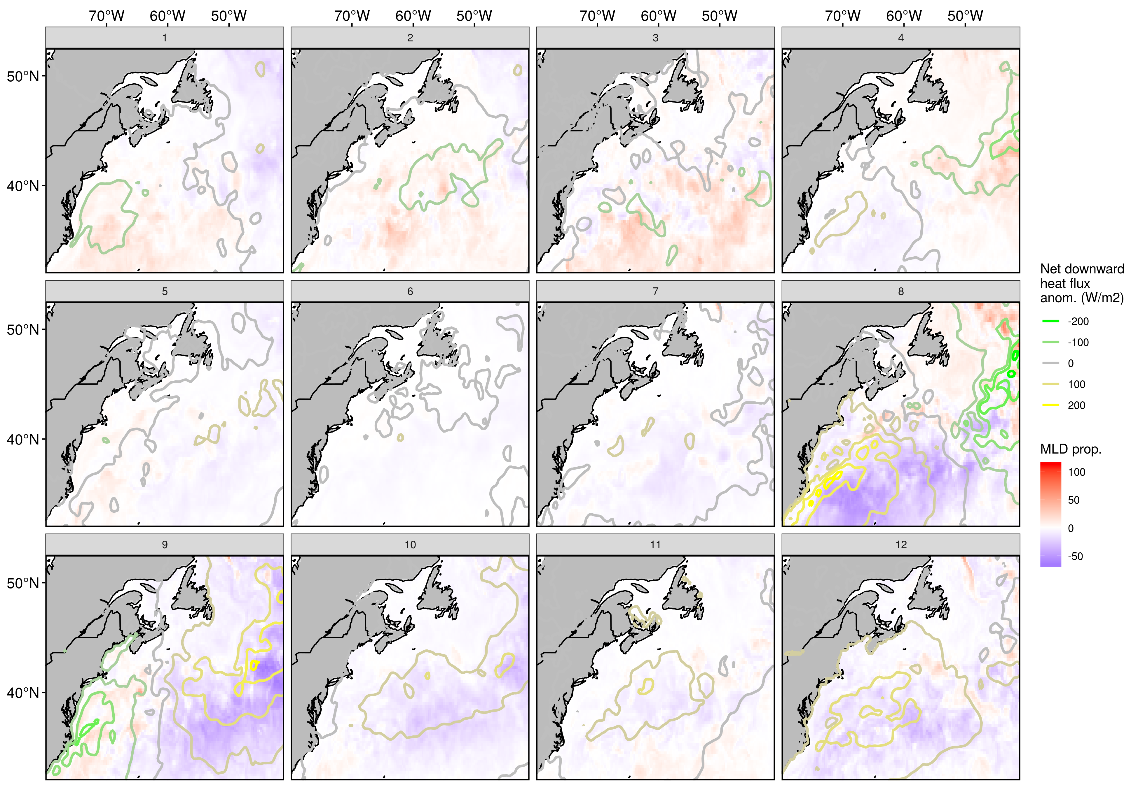
MLD + Net downward heatflux
The MLD in the AO in the top nodes is generally deeper, and shoals as we move to the bottom row. The MLD in the LS is deeper in the right-hand column and shoals as we move left. The MLD for the mab is deeper in the left-hand column and shoals as we move to the right.
The gradients of net downward heatflux change nicely across the nodes and generally speaking we see more positive downward heatflux over areas with anomalously shallow water. There is little happening in the centre two nodes. There is high positive downward heatflux over the LS in the bottom left node (9) with negative heatflux over the mab. This positive heatflux gradient slowly moves over the AO as we move from the left to the right along the bottom row of nodes. There is a negative downward heatflux gradient over the mab in the top left node (1) that slowly moves up and over to the LS as we move towards node 4. This negative gradient is replaced by a positive gradient.
Expand here to see past versions of fig_4.png:
| Version | Author | Date |
|---|---|---|
| 9273f18 | robwschlegel | 2019-08-11 |
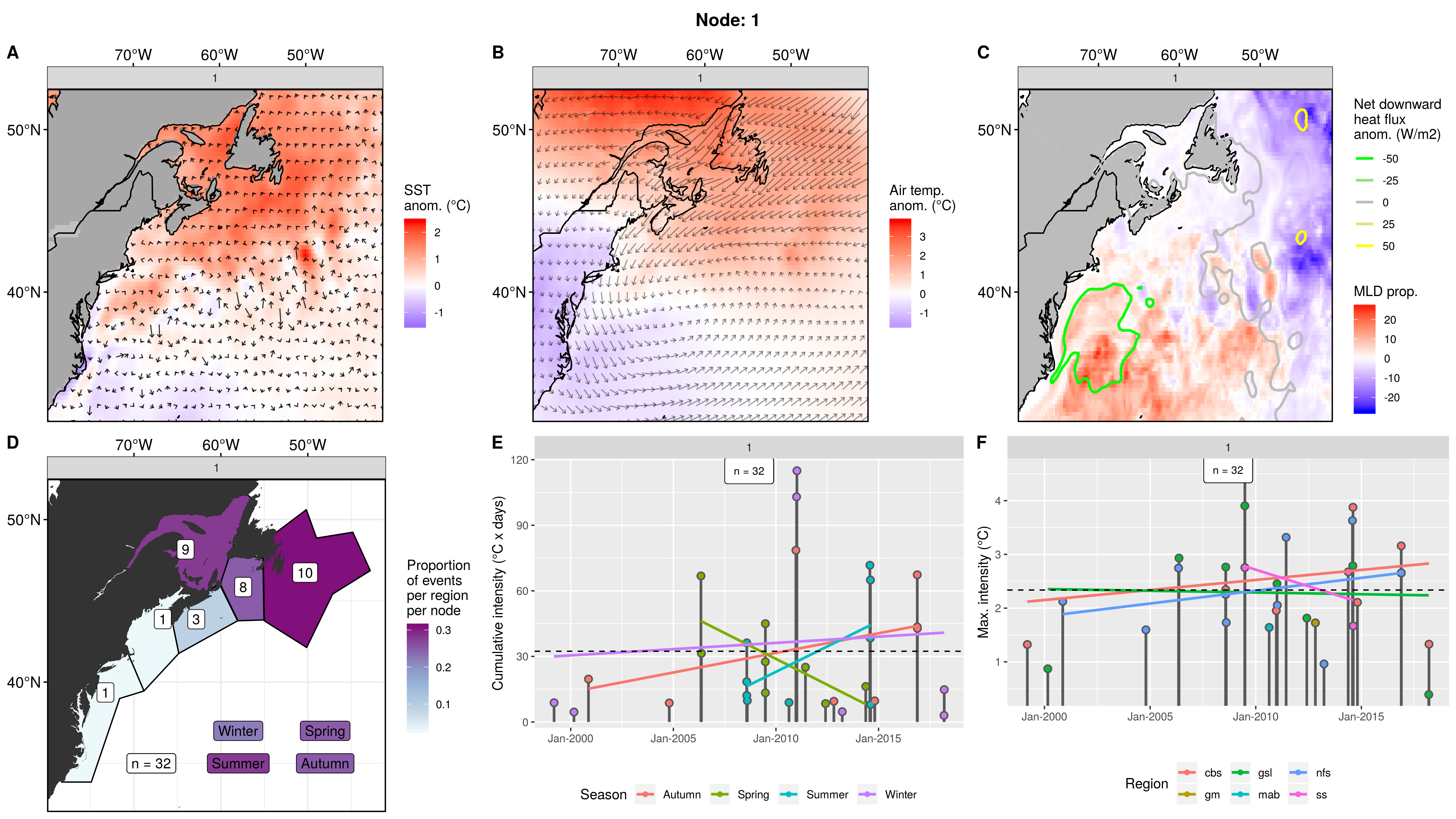
Node 1
This node has a pretty even split of months of occurrence, with a lean towards summer and away from winter. Most of the events took place in the nfs, cbs, or gsl. The most intense events in this node occurred in Autumn/Winter of 2010/11. There are events from 1999 to 2017 with more events in the later half. There is a big mix of very small and somewhat large events for both cumulative and max intensities.
The Southeast AO tends to be cold with a warm GSL and LS. Looking closely one may see that the GS is slightly anomalously slow. The atmosphere is dominated by a cyclonic dipole offshore of the mab/gm. The Southeast AO is up to 20 metres deeper than usual with a negative downward heatflux over it. The LS is shallow but there is not much positive heatflux into it, with the exception of two curiously concentrated points.
Expand here to see past versions of node_1_panels.png:
| Version | Author | Date |
|---|---|---|
| 9273f18 | robwschlegel | 2019-08-11 |
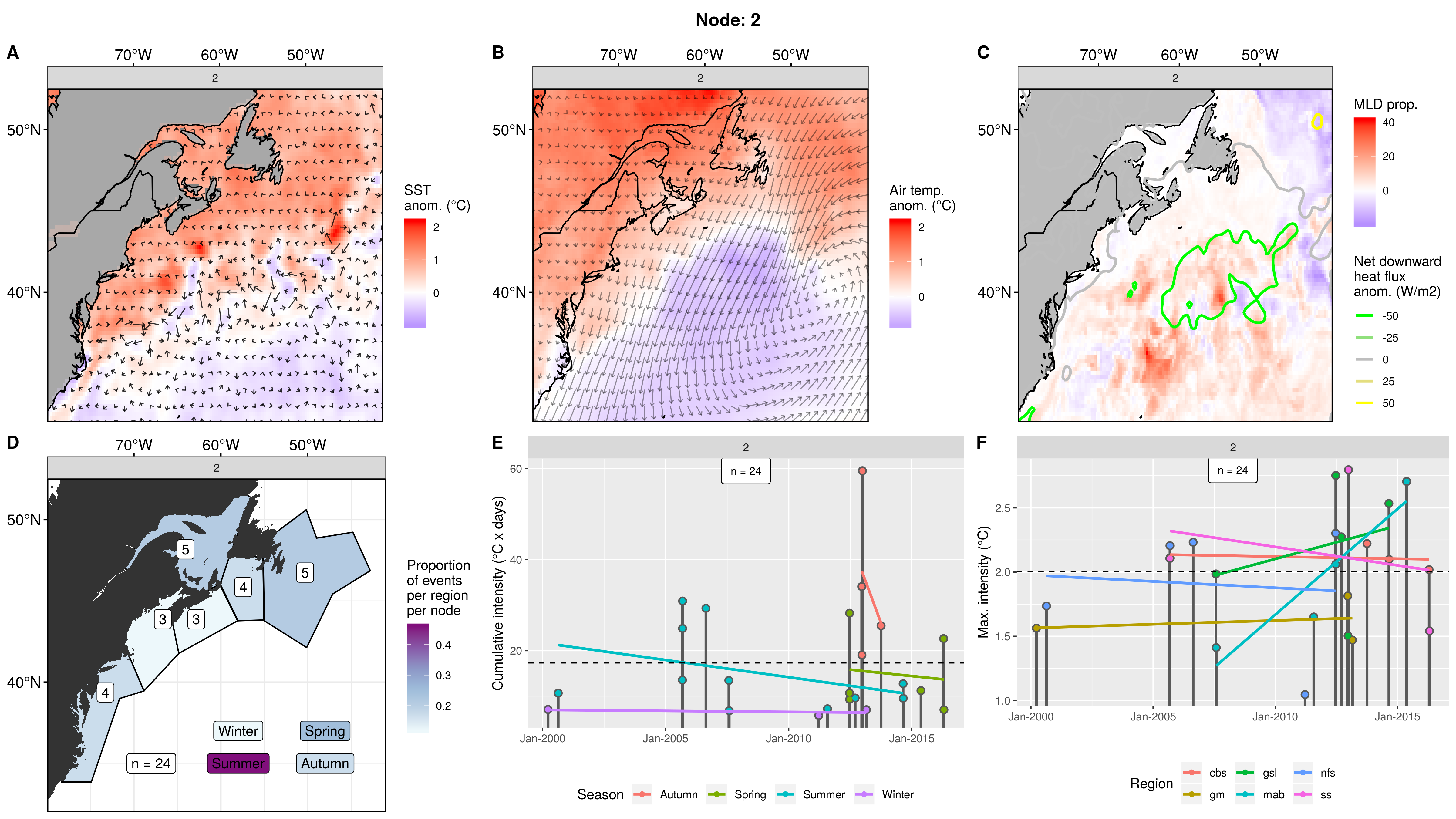
Node 2
A very even distribution of MHWs across all regions. Mostly summer then spring. The occurrence of events spans 2000 to 2016, with the most intense event in 2012. The cumulative and max intensity of these events are very low. The occurrence of these events in autumn happened only twice, 2012 and 2013. When these events occur in winter they have a cumulative intensity of ~10. lol.
A cold AO with a warm yet very turbulent GS with many warm/cold core eddies. It is surprising how well the detail of the eddies comes through given that these are many different events over many years. The rest of the coastal waters and LS are all warm with relatively little movement. Air over AO is cold but warm everywhere else. Strong cyclonic wind anomalies over the area south of where the AO and LS meet. No wind movement over land where the air anomaly is warmest. Positive heatflux over LS, where MLD is slightly shallow. Negative heatflux over deeper AO/GS where it is approaching the LS. The many eddies show up here in a more unusual MLD pattern, too.
Expand here to see past versions of node_2_panels.png:
| Version | Author | Date |
|---|---|---|
| 9273f18 | robwschlegel | 2019-08-11 |
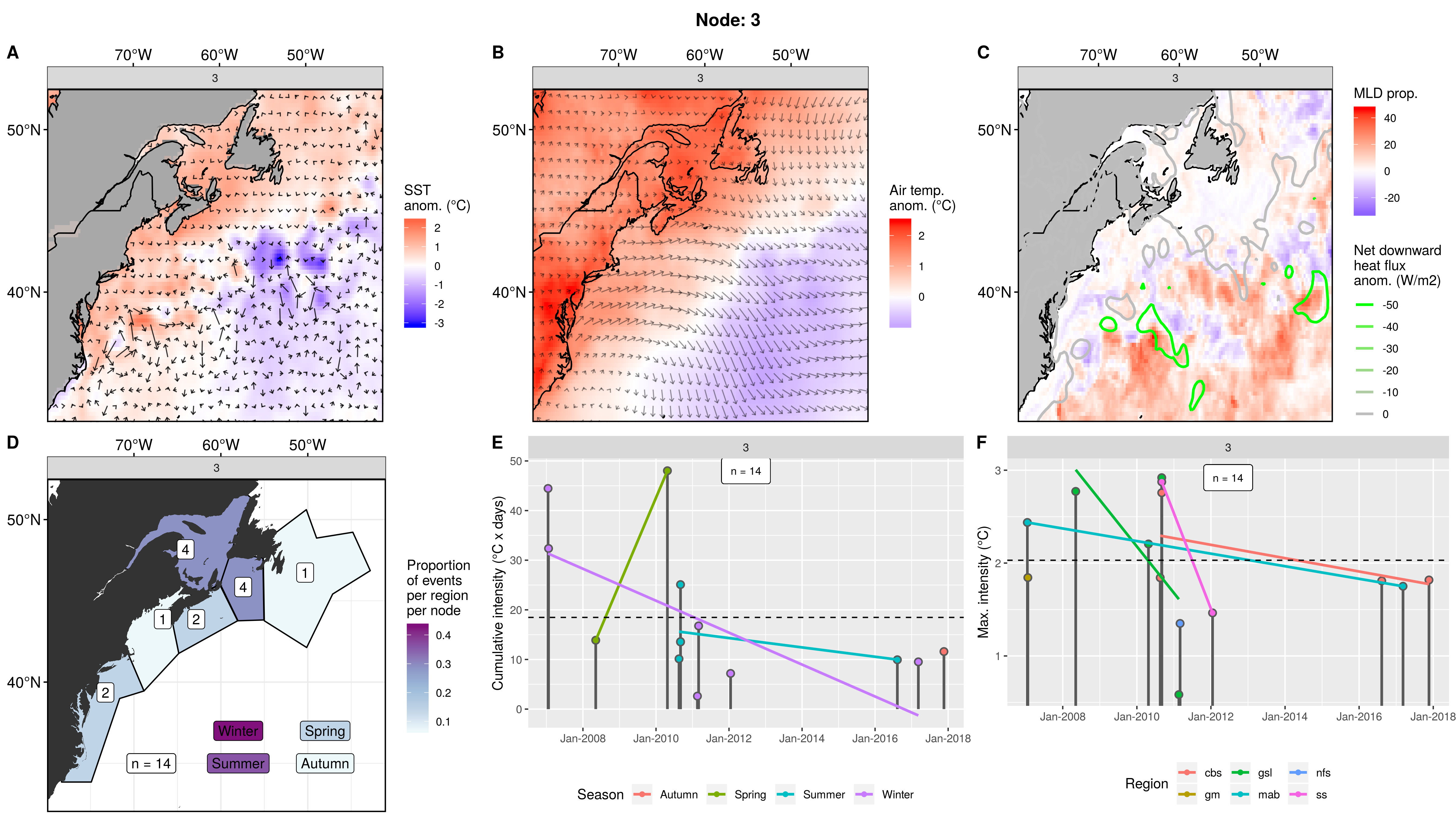
Node 3
Almost half of these events occur in winter, with most of the rest in Summer some how. There are about half as many MHWs in this node than normal at a count of 14. Most events occurred in the gsl and cbs. The occurrence of events spans only 2007 to 2017, with most events occurring in the first half.The cumulative intensities are very low, but with normal max intensities.
Cold (warm) eastern (western) AO with warm water everywhere else. Strong eddies in the GS. There appears to be an anticyclonic cell pulling warm air up the coast and cold air over the AO. But there is also a cyclonic cell in the northeast corner that appears to be doing the same. There is little warm air movement inland. There is no positive heatflux in this node, and relatively weaker heatflux over some of the deeper MLD associated with eddies. Slightly shallower water in the coastal regions.
Expand here to see past versions of node_3_panels.png:
| Version | Author | Date |
|---|---|---|
| 9273f18 | robwschlegel | 2019-08-11 |
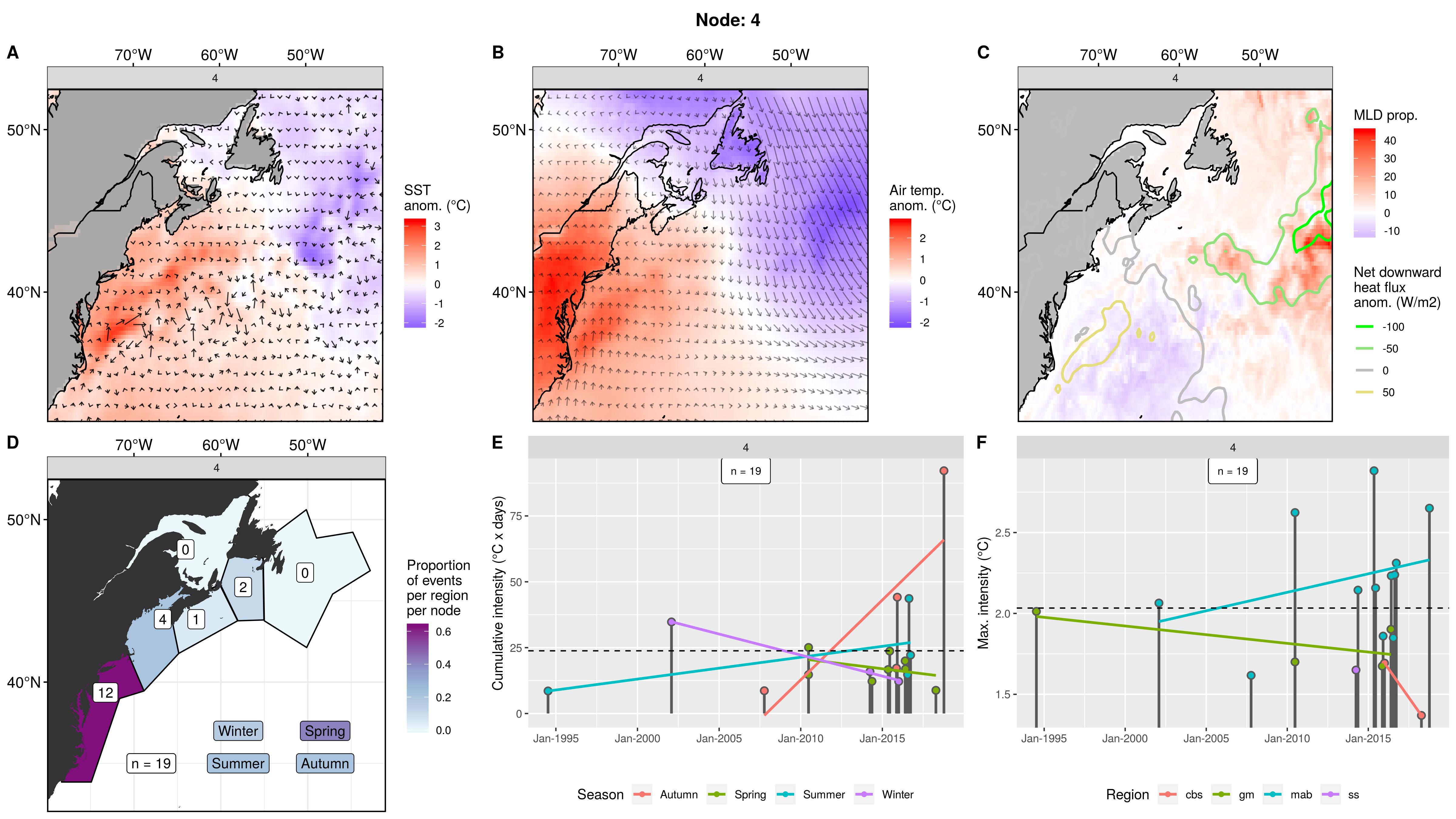
Node 4
These MHWs occurred almost entirely in the mab with a bit trailing out into the gm, ss and cbs. Half of the events occurred in Spring, with the other half split between the other three seasons. Low cumulative intensities, but mid-high max intensities. The MHWs that occurred in the mab tend to have higher max intensities.
Very clearly a strong + warm GS pushing up closer along the shelf during a cold LS. Warm air anomalies over US and GS with strong northward wind anomalies. Cold air over CN with southward air anomalies. These two air flows appear either unconnected or perhaps two separate cyclonic and anticyclonic cells. Positive heatflux into shallower GS with a strong negative flux into deeper point where the LS and GS meet.
Expand here to see past versions of node_4_panels.png:
| Version | Author | Date |
|---|---|---|
| 9273f18 | robwschlegel | 2019-08-11 |
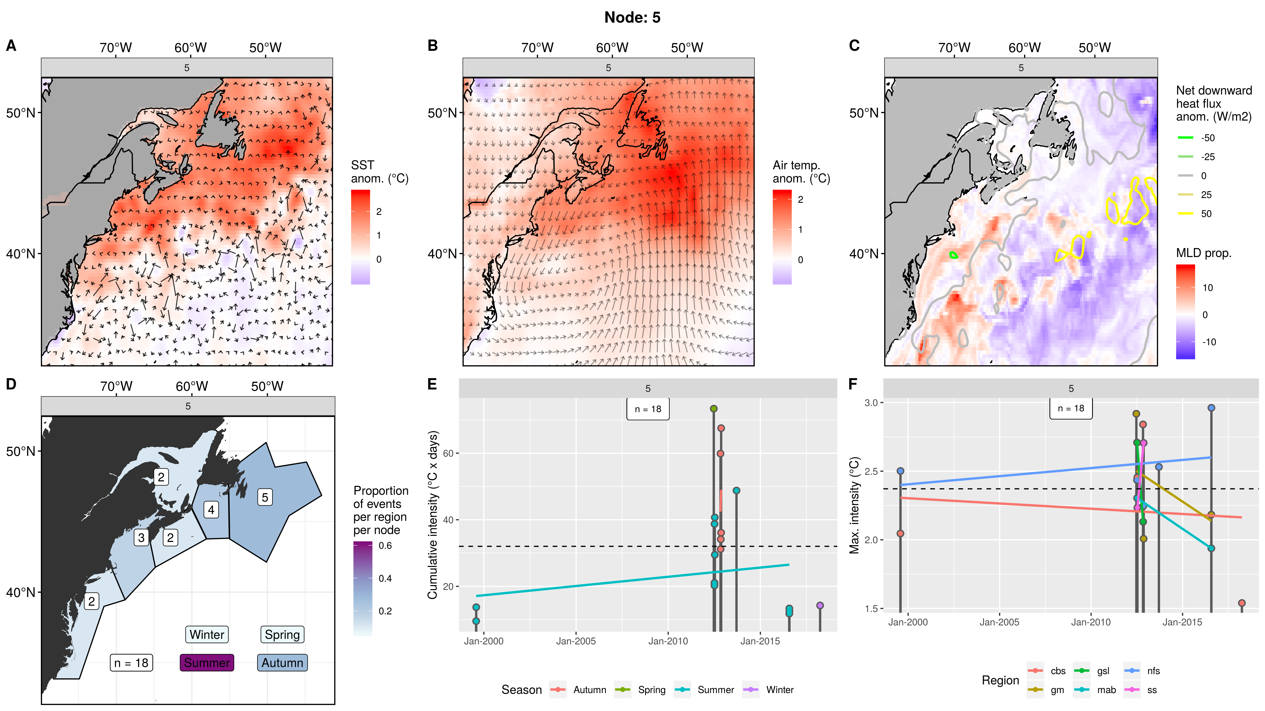
Node 5
These are very much summer events, with a bit spilling out into autumn and only one event in spring and winter. Most events occurred between 2012 to 2017. Two small events occurred in 1999. Low cumulative intensities but relatively high max intensities. The intensity of events in the autumn are greater than the summer. This could be due to phenology shifts of this storm pattern.
Cold AO and GS with very turbulent eddy field. Warmer SST anomaly everywhere else. Warm air anomaly over nearly all of the study area, hottest over the grand banks. Large cyclonic cell sitting over area where GS pulls away from coast. Slightly deeper MLD of waters along coast, possibly due to GS. Also slightly deeper MLD in GS at bottom of study area and in some eddy cores. Some small negative heatflux into mab/gm waters, and some positive heatflux out of GS as it travels out of the study area. Nothing remarkable.
Expand here to see past versions of node_5_panels.png:
| Version | Author | Date |
|---|---|---|
| 9273f18 | robwschlegel | 2019-08-11 |
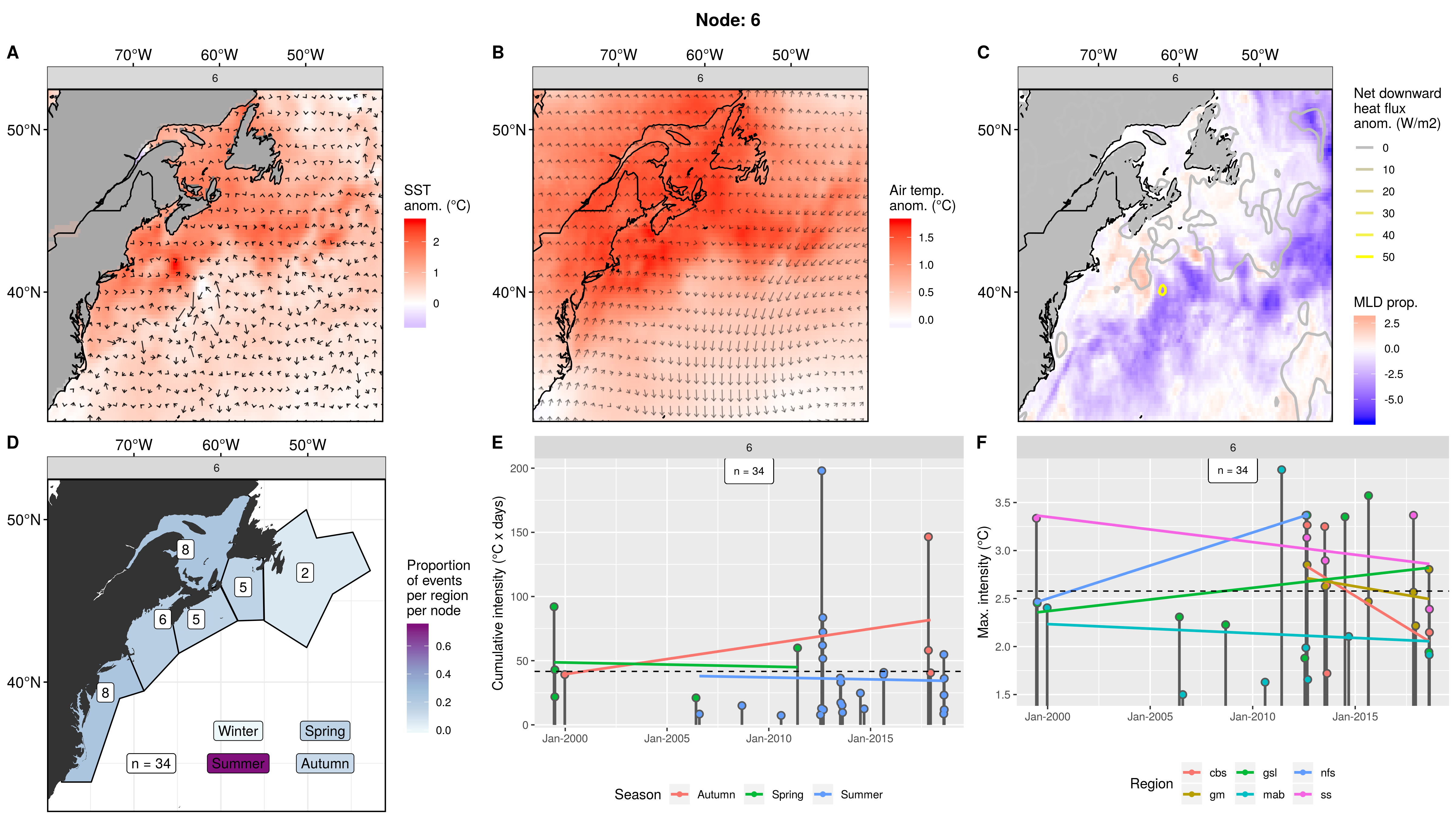
Node 6
A node with many MHWs clustered into it. An even number (8) of MHWs occurred in the mab and gsl, which is a bit strange. A couple less in the gm, ss, and cbs. Only two in the nfs. Almost all of the events occurred in summer, with 4 in autumn and 5 in spring. The cumulative intensities are medium high with a couple of very large MHWs. The max intensity on these events is very high on average, with several medium sized ones.
Warm SST and air anomalies throughout entire study area. Note that the air temp anomalies are actually low, at less than 2.0, compared to most of the other nodes. Very little current anomaly and some faster northward air over US coast while some southward wind anomaly over AO. Wind in the north of the study area has slight northward anomaly. Very little happening w.r.t. MLD and heatflux. It is worth noting that there is no negative heatflux, and little positive heatflux.
Expand here to see past versions of node_6_panels.png:
| Version | Author | Date |
|---|---|---|
| 9273f18 | robwschlegel | 2019-08-11 |
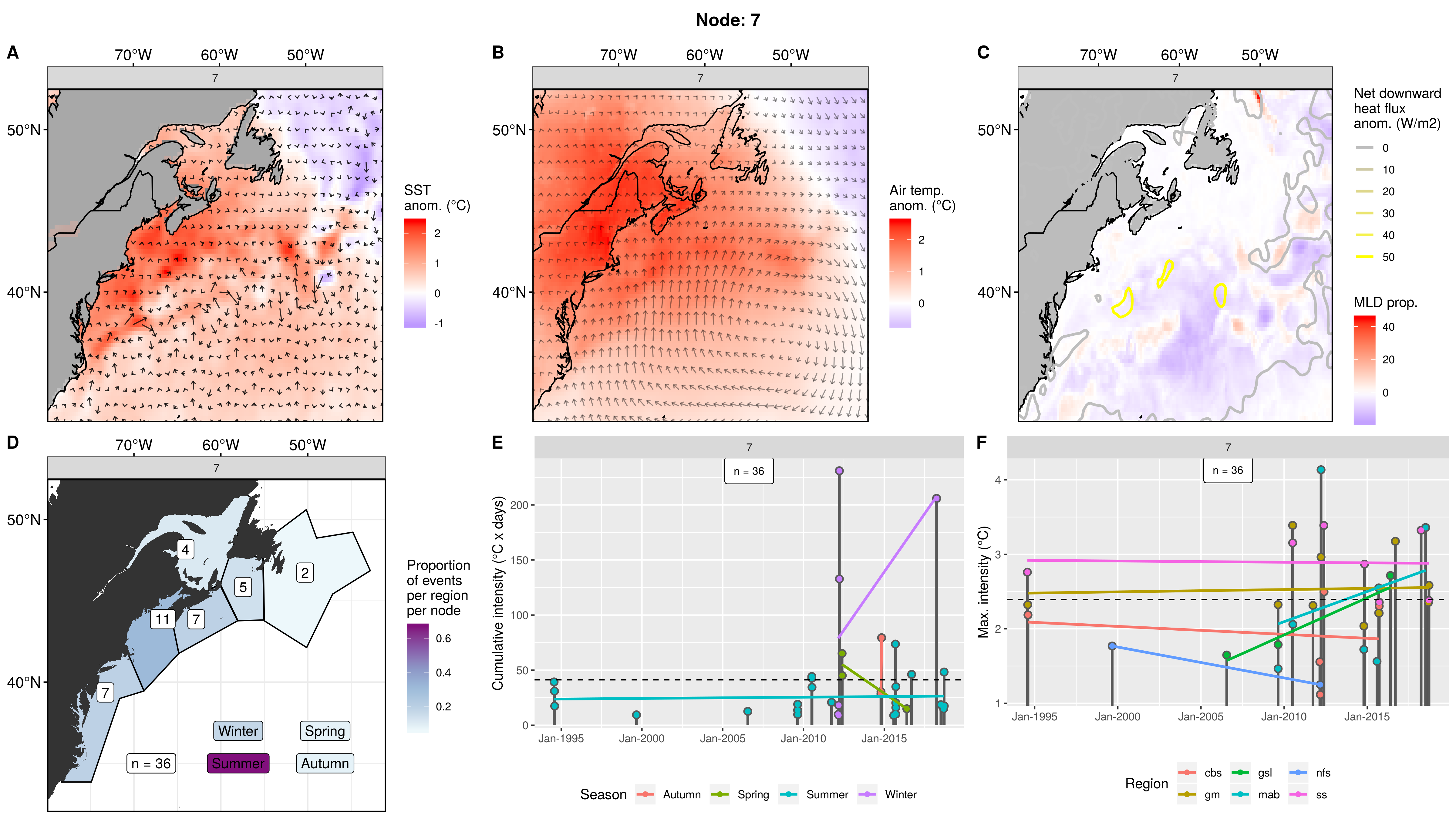
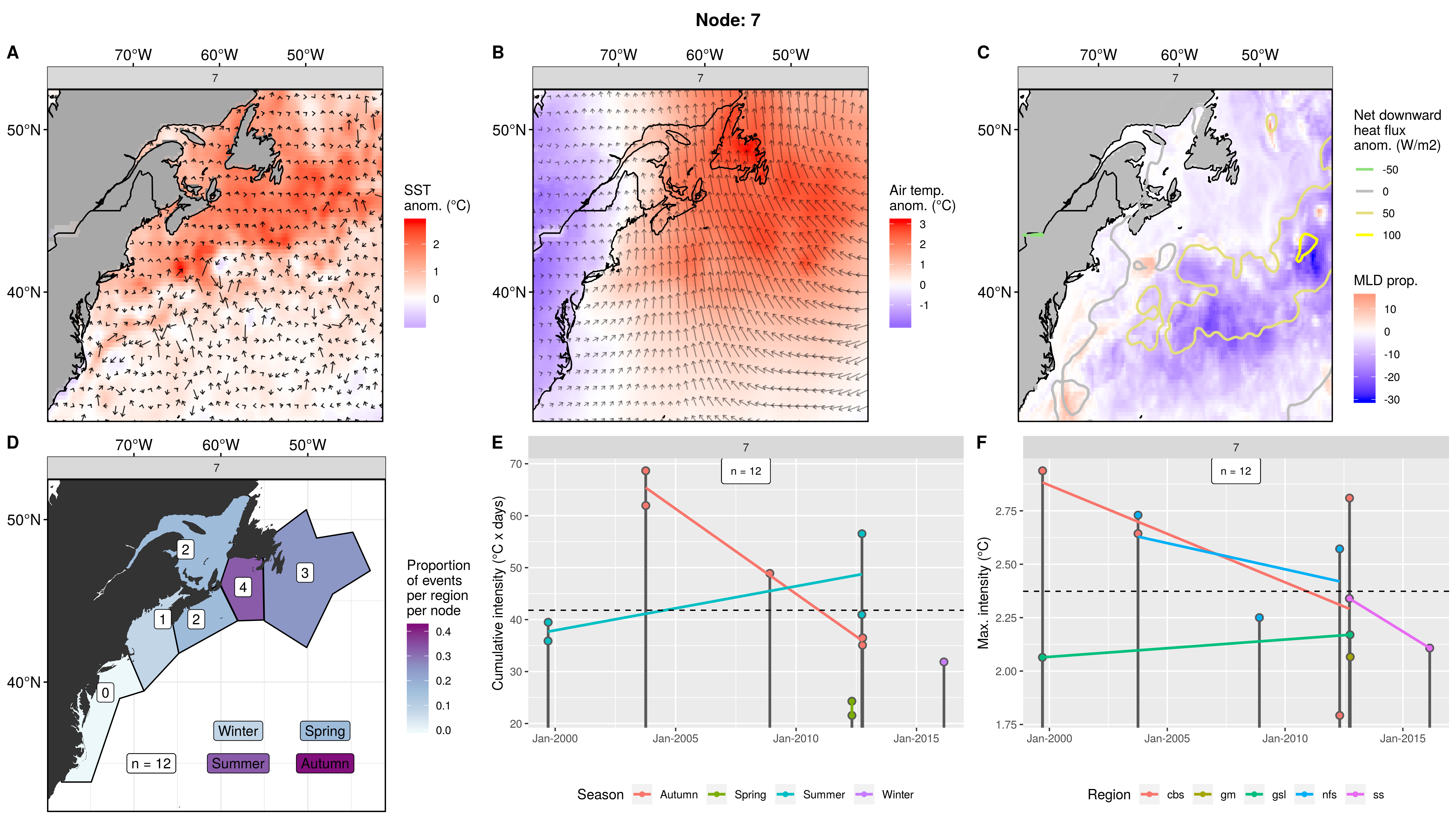
Node 7
Roughly three quarters of events occurred in summer. Highest centre of occurrence in the gm at 11 MHWs, slowly decreasing count of MHW as one moves further away from the gm region, with only two MHWs in the nfs. Even though this is a mostly summer node, the summer events are small at a mean cumulative intensity of ~30. The MHWs in other seasons tend to be larger, with 3 of the 5 winter MHWs that occurred here being massive. The max intensity of events here and medium to very high, with one winter being over 4C! Events occurred like this from 1994 to 2017, but things really started to pick up in 2012.
A slightly warm AO with a stronger GS and warm coastal waters but cold LS. Warm air over US - CN border with large anticyclone cell over eastern AO. Possibly drawing down colder air from the LS. Some pockets of deeper MLD likely due to eddies. Some positive heatflux and no negative heatflux. It’s strange that the maximum intensities are so high while the heatflux anomalies are low. The air and SST anomalies are higher than most nodes though.
Expand here to see past versions of node_7_panels.png:
| Version | Author | Date |
|---|---|---|
| 9273f18 | robwschlegel | 2019-08-11 |
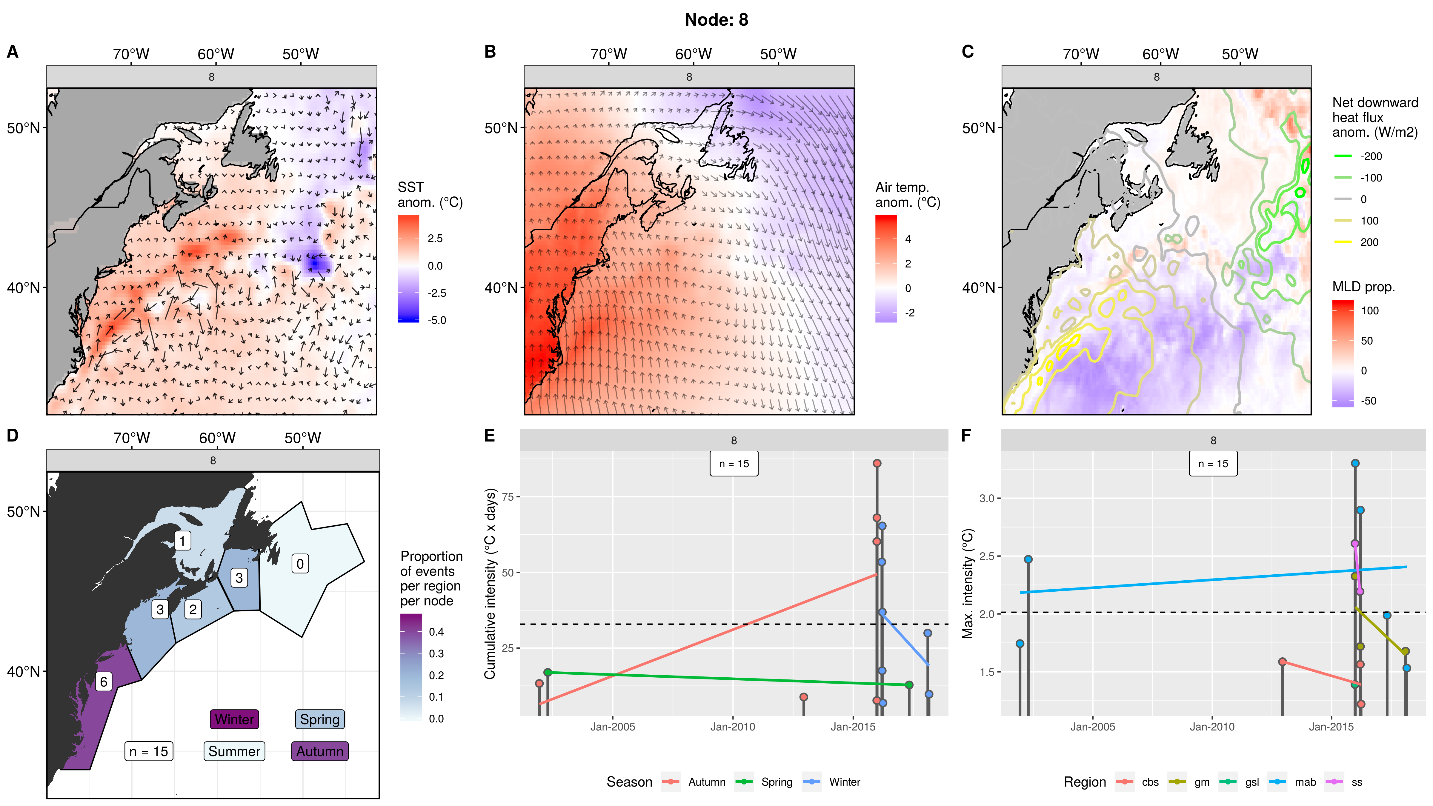
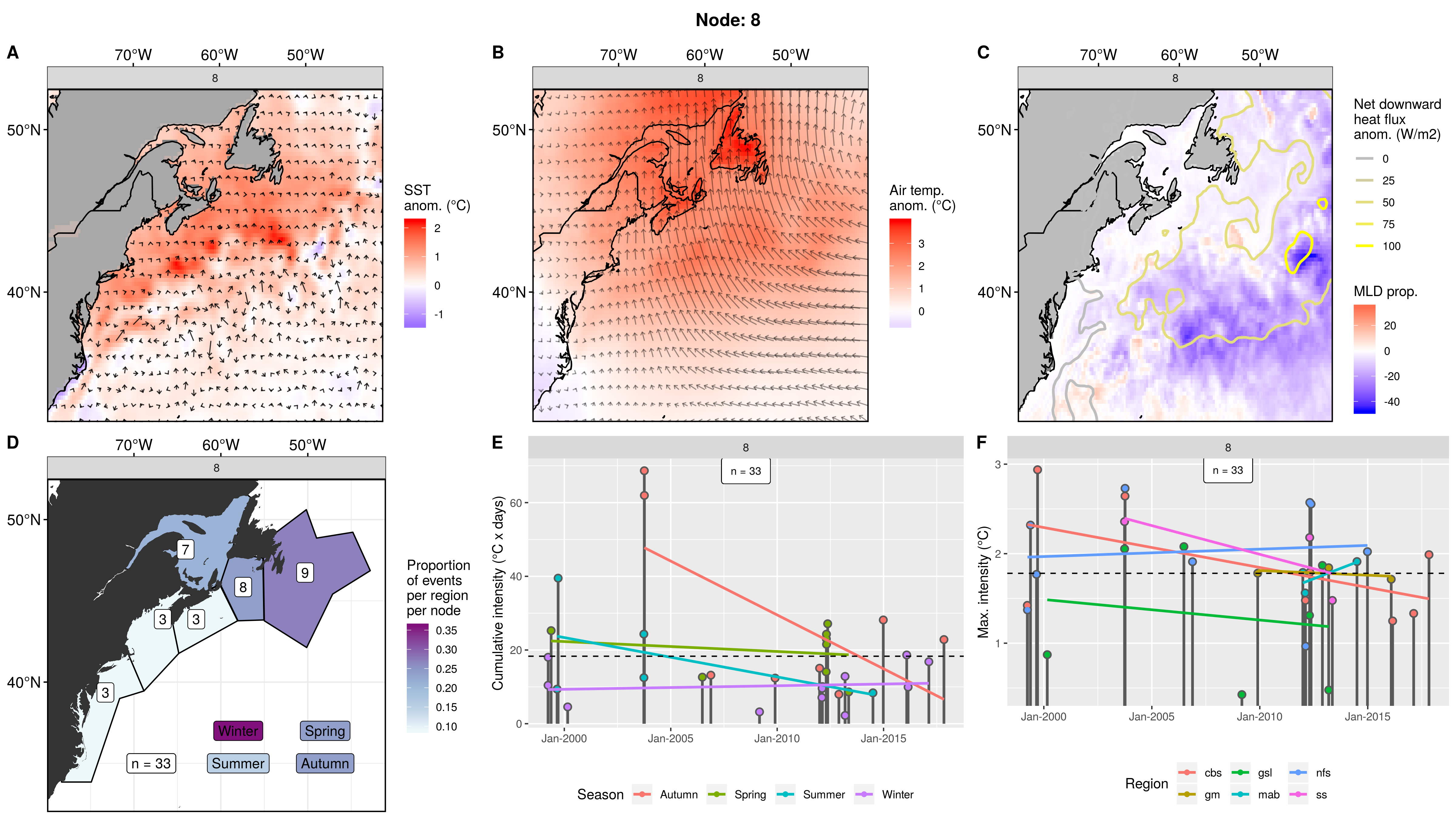
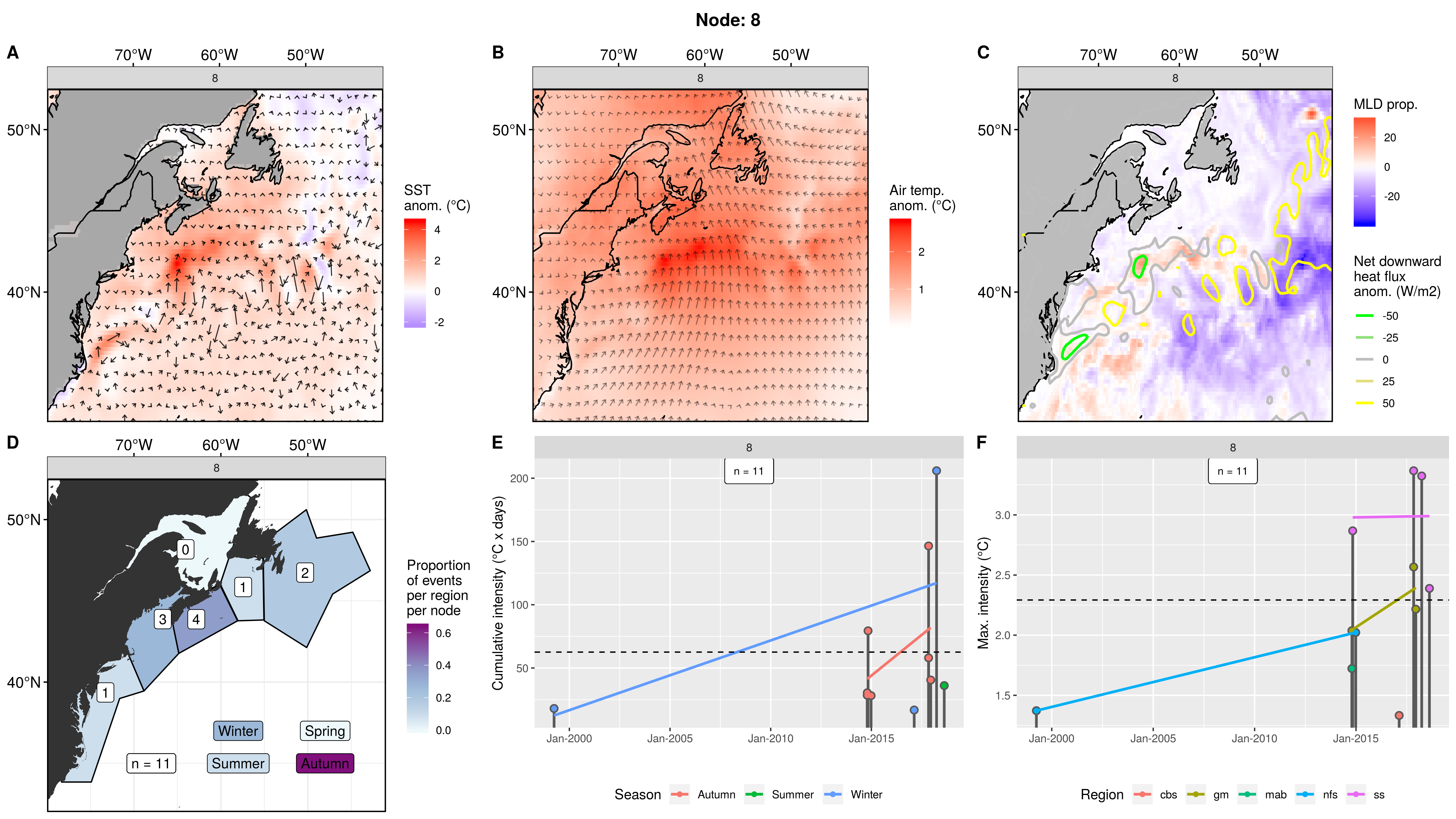
Node 8
This node has only 15 MHWs clustered into it. Almost half of the MHWs occurred in the mab, with fewer in the other coastal regions, only one in the gsl, and 0 in the nfs. The main range of MHWs occurred from 2015 - 2017, with two small events in 2003 and one even smaller event in 2012. This node primarily consists of two events that occurred over autumn and winter of 2016. Most of the other smaller events from years outside of that occurred in the mab.
Obviously strong coast-ward GS with a strong eddy field. High SST anomaly with a super cold core anomaly to the east. Crazy high (~5C) air anomaly over US and GS with concurrent northward winds. Cold southward flowing air from over the cold LS waters. It doesn’t really look like this is one weather system, rather two. Crazy high positive heatflux (~200W/m2) over GS near the coast and very shallow AO, with equally massive negative heatflux over very deep LS. The heatflux anomalies in this node are roughly 4 times larger than most other nodes. Something hectic is happening here but I’m not quite sure what it is.
Expand here to see past versions of node_8_panels.png:
| Version | Author | Date |
|---|---|---|
| 9273f18 | robwschlegel | 2019-08-11 |
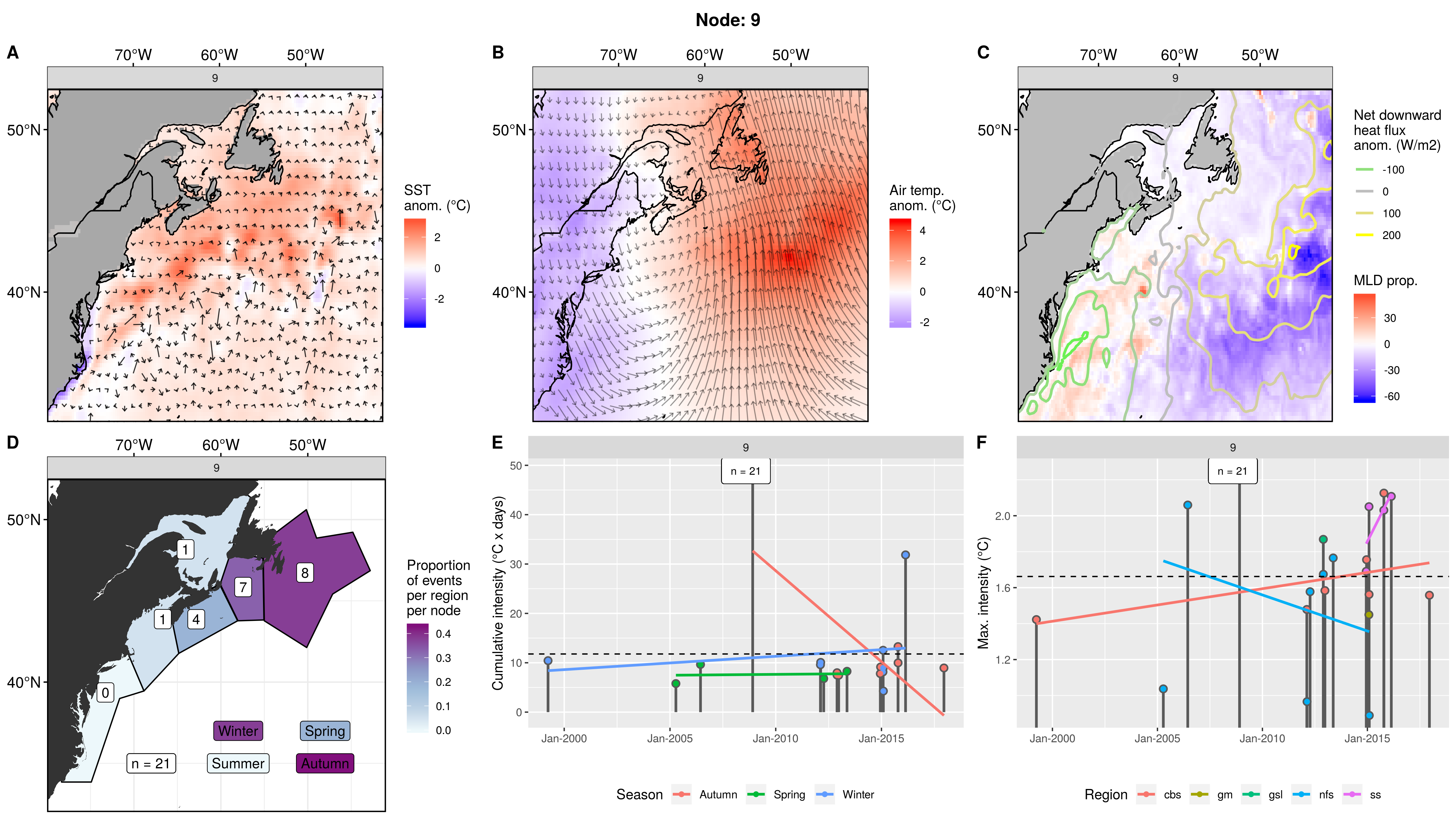
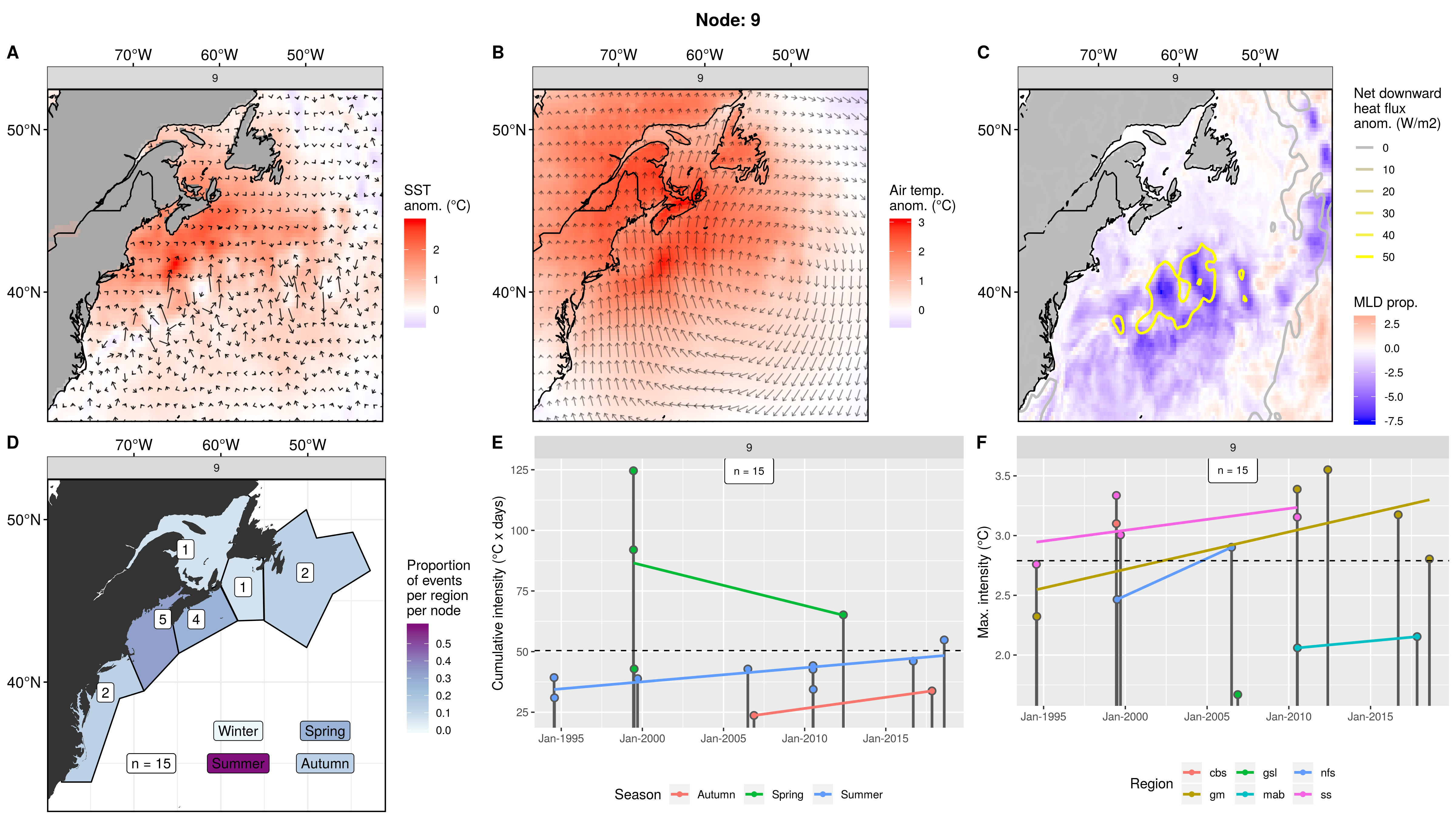
Node 9
Most MHWs occurred here in autumn and winter in either the nfs or cbs, with 4 in the ss. MHW occurrences range from 1999 to 2017. These MHWs are very small.
Cold GS along coastline, with warm waters everywhere else. GS is moving a bit more quickly with some good eddy action. Cold southward air over CN, US, and GS. Very warm northward air over AO + LS. Strong negative heatflux over shallow GS with massive positive heatflux into much deeper AO + LS.
This is very clearly a cyclonic system moving up the coast bringing warm air out to the nfs and pulling cold air down over the mab and gm.
Expand here to see past versions of node_9_panels.png:
| Version | Author | Date |
|---|---|---|
| 9273f18 | robwschlegel | 2019-08-11 |
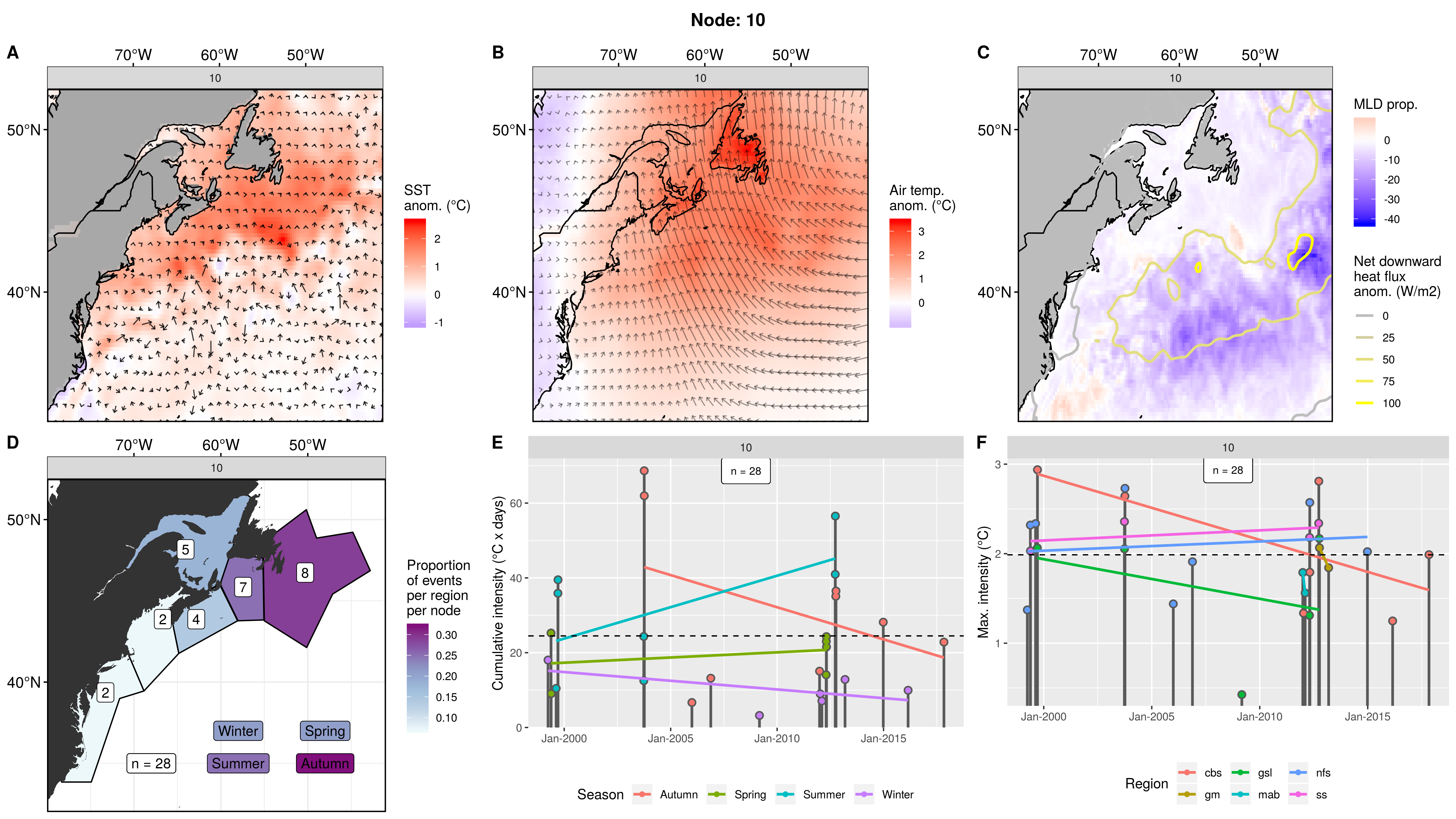
Node 10
About 1/3 of events occurring in the nfs, and decreasing as one moves further away. About one third of events occurred in autumn and a normal spread to the other seasons. The MHWs occurred from 1999 to 2017. The MHWs in this node stand out a bit in that they occurred a bit more in concentrated clumps than usual. Meaning that we see multiple regions experiencing MHWs at the same time. The cumulative intensities are low but the max intensities are lo-medium to high-medium. There is an even spread of events over time.
We see a mostly warm SST anomaly everywhere but much higher over the nfs. Slight cold anomaly in GS near coast. Very mild cold air over US + CN with very high warm anomaly over nfs. There appears to be a warm massive anticyclone centred over the LS but reaching down into the AO. Very little positive MLD to be found, with a very shallow MLD for the AO and LS, but normal over the nfs.Large positive heatflux into he AO + LS.
This looks like some sort of huge tropical storm coming from the east to bring warm air to the nfs.
Expand here to see past versions of node_10_panels.png:
| Version | Author | Date |
|---|---|---|
| 9273f18 | robwschlegel | 2019-08-11 |
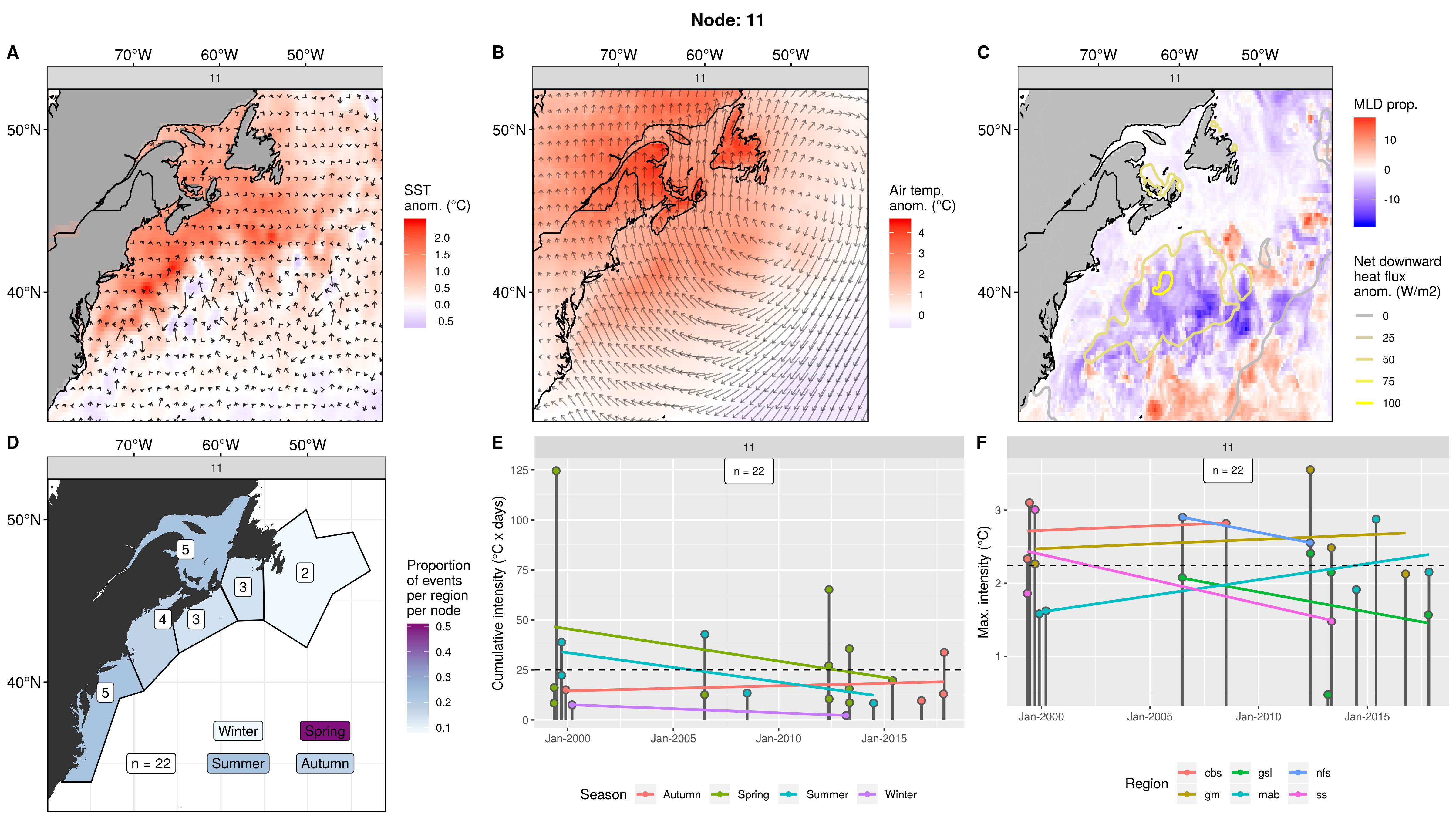
Node 11
Relatively even spread of events with more in the mab and gsl. Half of the events occurred in spring. The range is from 1999 - 2017 and well spread out. The largest MHW was in the cbs in 1999. Overall low cumulative intensities but medium to high max intensities. The winter MHWs are the smallest, with the spring and then summer events being the largest.
Mix of slightly warm and cold eddies in GS. Warmer waters to the north of the GS but less so in the LS. A very large anticyclone over the cbs + nfs that is pulling warm air up onto the coast where it reaches nearly 5C over CN. Slightly deeper southern AO and GS eddies with most of the rest of the study area being slightly shallow. No negative heatflux and strong positive heatflux over AO, with some very strong localised heatflux within the gsl and nfs.
Expand here to see past versions of node_11_panels.png:
| Version | Author | Date |
|---|---|---|
| 9273f18 | robwschlegel | 2019-08-11 |
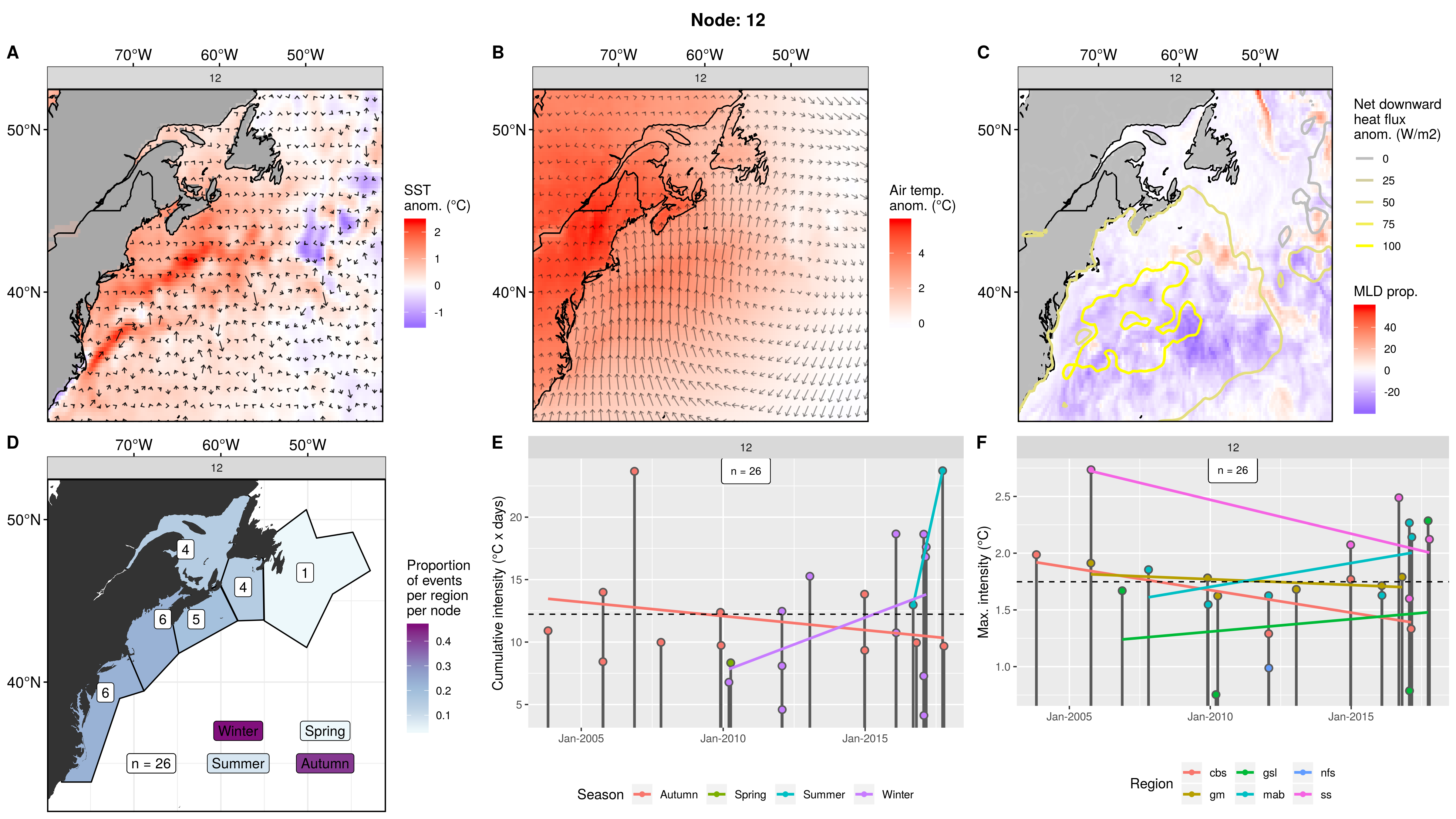
Node 12
An even spread between all regions except only 1 MHW in the nfs. Slightly fewer in gsl and cbs. Almost all events occurred in autumn and winter, with only 1 spring event and 2 in summer. Range is 2003 - 2017. These events are tiny, but some have medium max intensities.
A warm gulf stream and coastal waters with spotty LS. Very warm air over US + CN with northward wind anomaly over the GS + AO. There appears to be an anticyclone happening over the entire study area, centred south of where the AO and LS meet. A generally shallower MLD for the GS and AO, with a deep tongue in the LS. No negative heatflux with high positive heatflux into GS + AO.
This appears to be a big wind cell that is sitting over the AO in autumn - winter that is pushing a bunch of warm air over and into the coastal regions, excluding the nfs as the colder LS appears to maybe be blocking this.
Expand here to see past versions of node_12_panels.png:
| Version | Author | Date |
|---|---|---|
| 9273f18 | robwschlegel | 2019-08-11 |
SOM experiment: Default, 3x3 nodes
Node summary table
The table below contains a concise summary of the nodes following Table 4 in Oliver et al. (2018). The following sub-sections provide more in-depth explanations.
| Node | Region | Season | MHW Properties | Conditions |
|---|---|---|---|---|
| 1 |
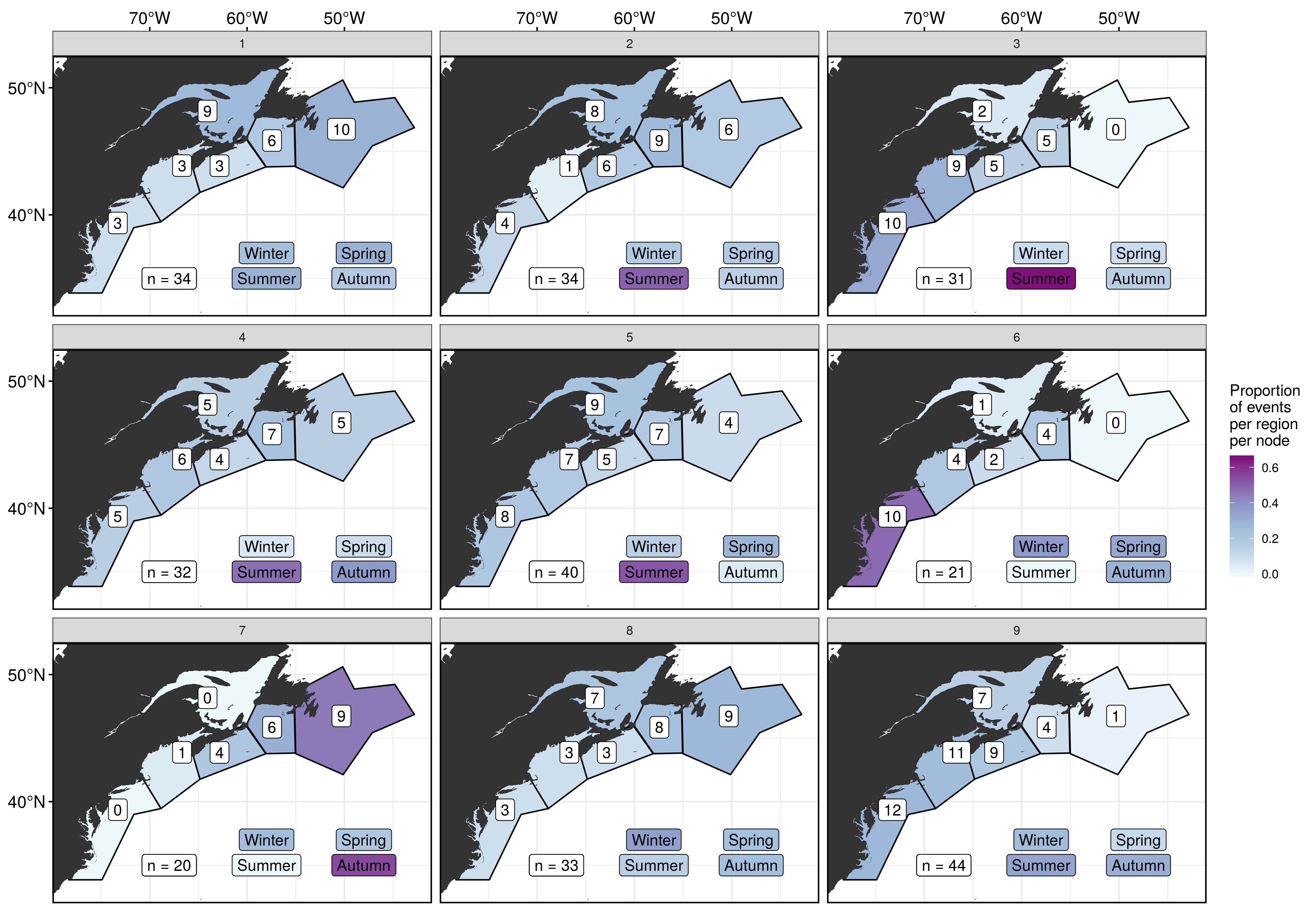
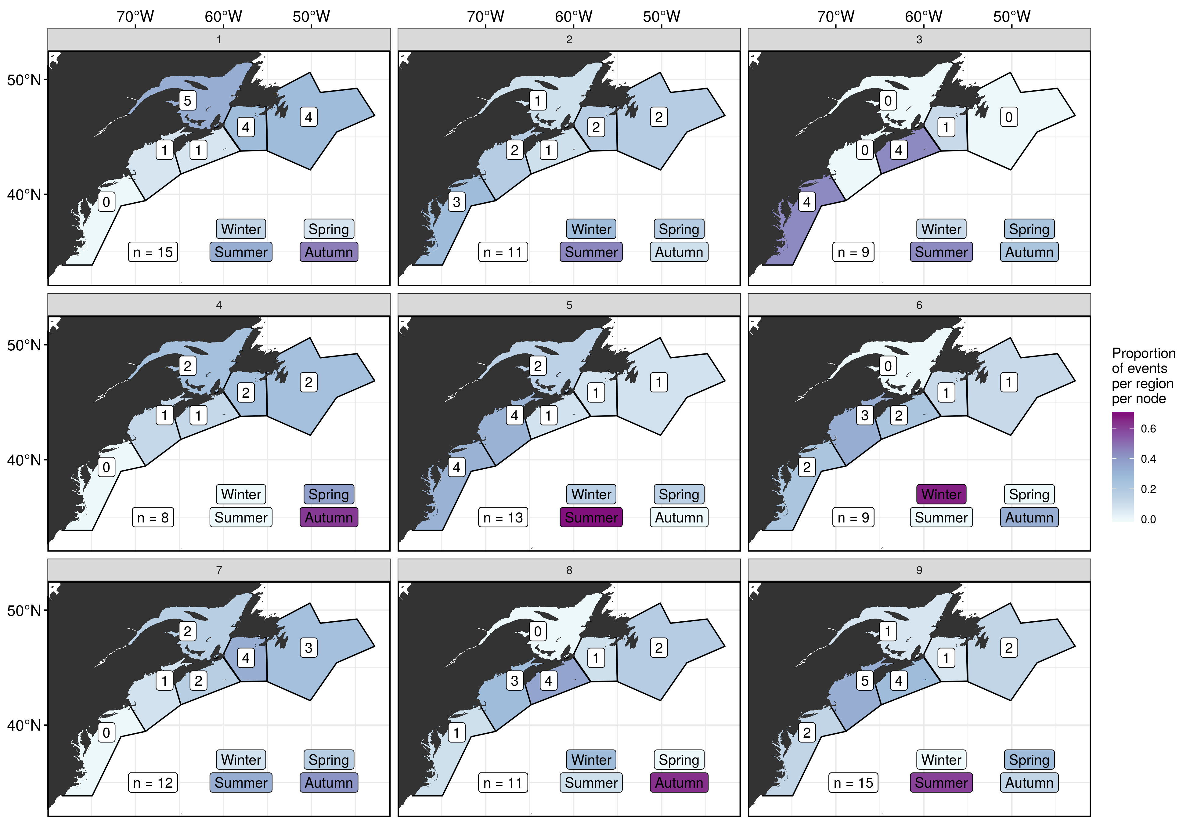
Season + region
The right-hand nodes (3, 6, 9) have (almost) no MHWs counted in the nfs, and generally show a higher proportion of events occurring towards the more southern regions. The middle nodes have a more even distribution of regions of occurrence, while the left-hand nodes are shifted more towards the nfs. There isn’t too clear of a pattern of the season of occurrence, but there is a line of largely summer months running through the middle of the nodes (4, 5, 2) and up out of the top right node (3). The bottom left node (7) has a high autumn proportion and the other nodes have a pretty even mix. There are almost no summer events in nodes 7 + 6, but these are not next to each other.
Expand here to see past versions of fig_5.png:
| Version | Author | Date |
|---|---|---|
| 9273f18 | robwschlegel | 2019-08-11 |
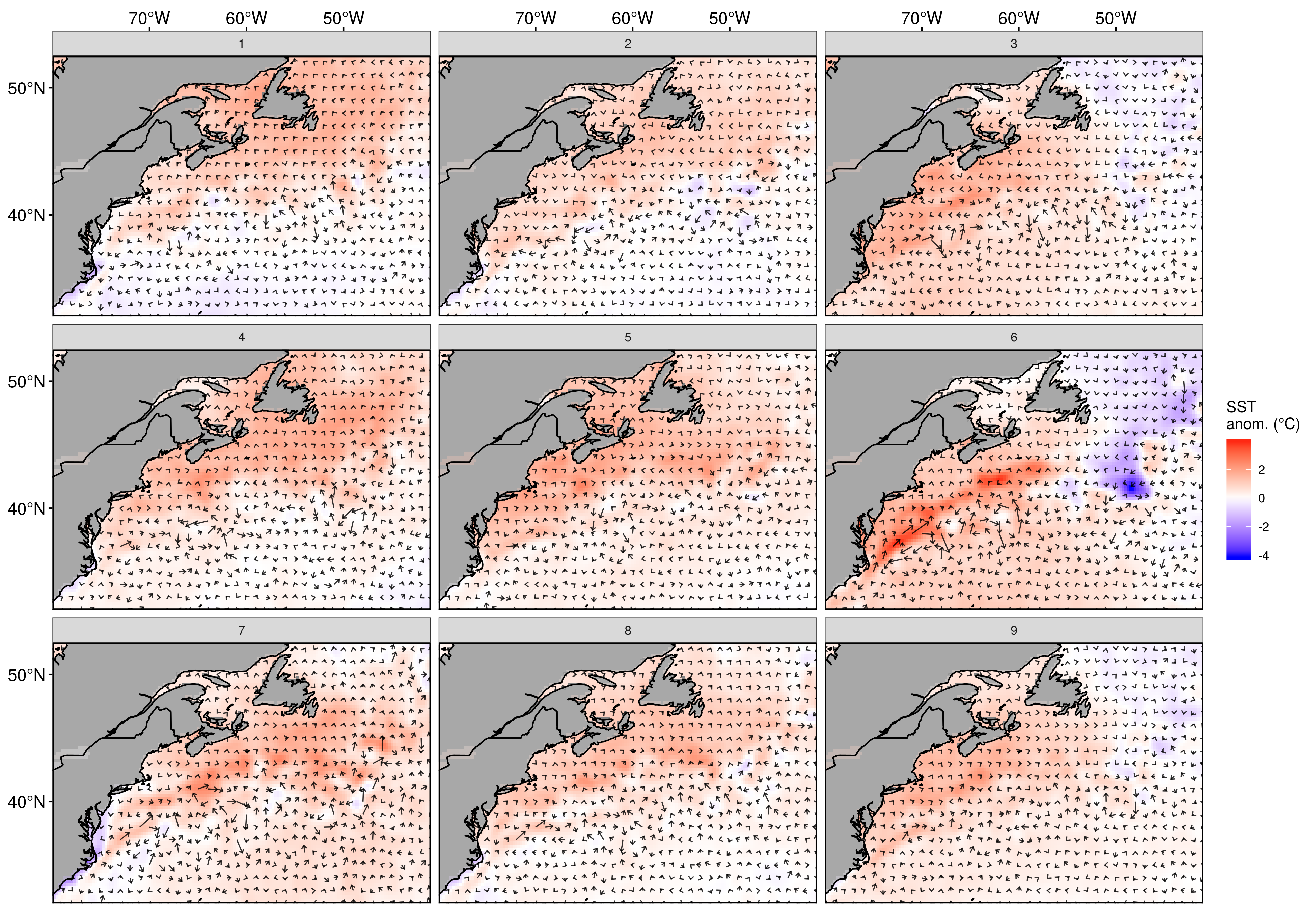
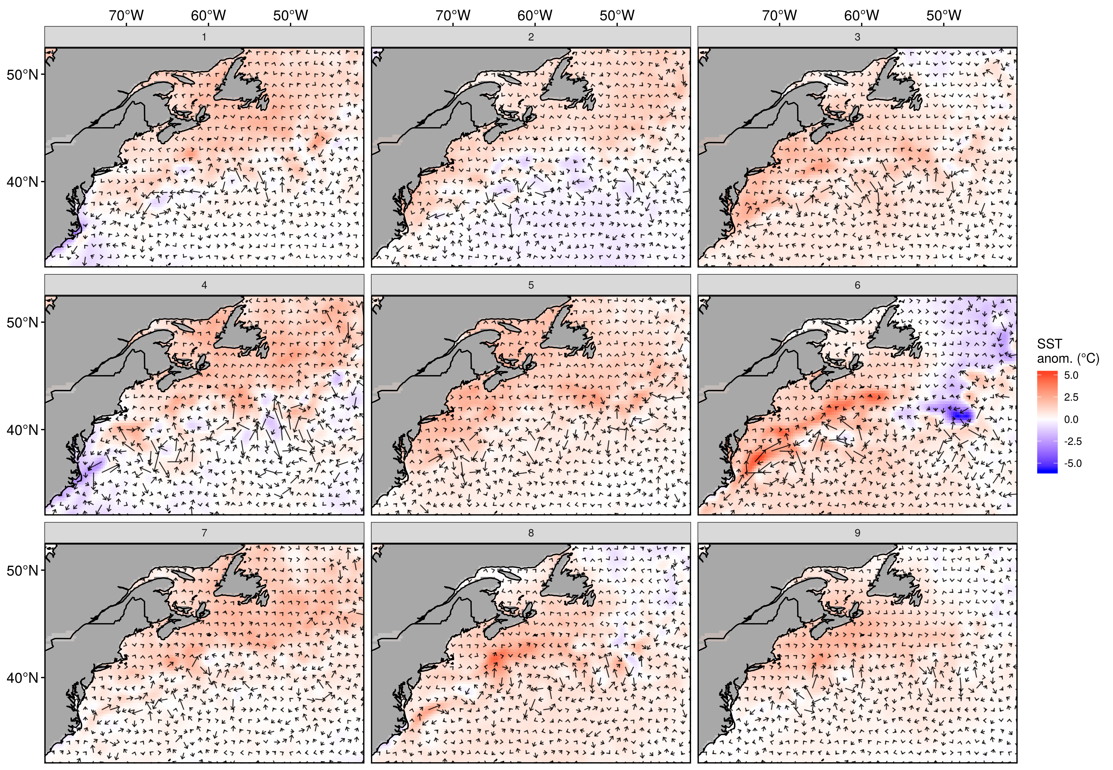
SST + U + V
We see a cooler LS on the right-hand side that arms up as we move to the left and up. The AO is cooler in the top left corner and becomes warmer moving right and down. Nodes 3, 6, and 7 show stronger GS movement.
Expand here to see past versions of fig_2.png:
| Version | Author | Date |
|---|---|---|
| 9273f18 | robwschlegel | 2019-08-11 |
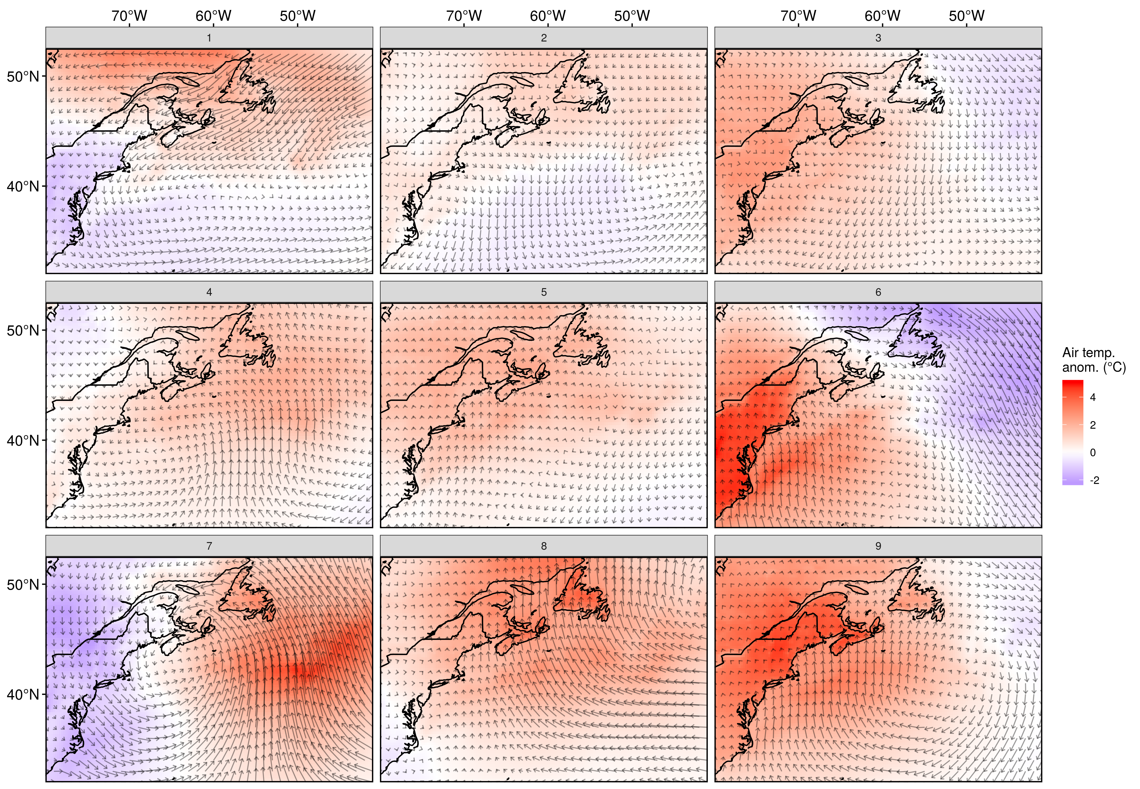
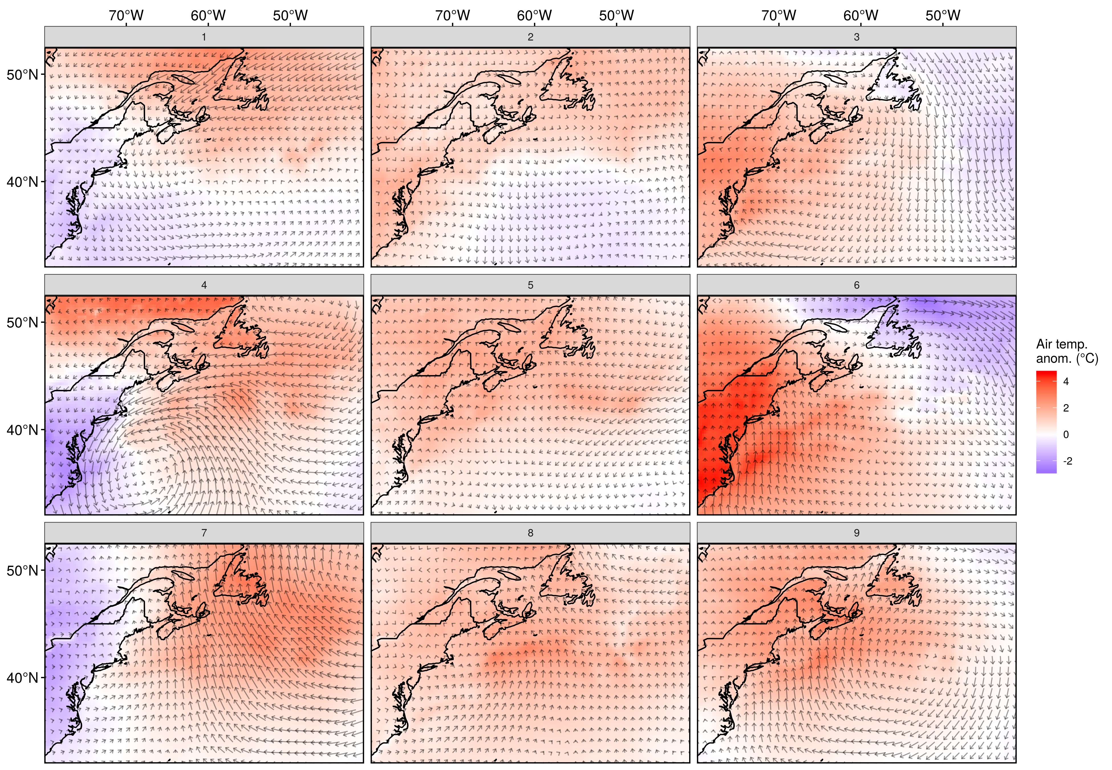
Air temp + U + V
Air over the LS is cooler on the right-hand column and becomes warmer to the left. Air over the AO is cooler in the top left and generally becomes warmer the further away the nodes are from node 1. Node 7 is interesting in that it shows a strong vertical dipole with cold air over CN, US, and GS. The middle node (5) has the least amount of air movement and yet we still see the vague traces of warm air moving north and cold air moving south. Node 1 shows some sort of crazy warm wind pumping south from over the LS pushing cold air down the US coast then out over the AO. Nodes 3, 6, and 9 show vaguely similar anticyclones exchanging hot air up the coast and cold air down. The pattern is strongest in the middle node (6) and the centre of the cell moves to the east as one moves down the column. Node 8 is similar to node 9 but with the cell moved even further east. Node 7 shows a strong cyclone with a thermal dipole between land and sea, with a very warm air anomaly over the AO/LS. Node 4 almost looks like two opposite rotating wind cells coming together over the AO to push warm air anomalously northwards.
Expand here to see past versions of fig_3.png:
| Version | Author | Date |
|---|---|---|
| 9273f18 | robwschlegel | 2019-08-11 |
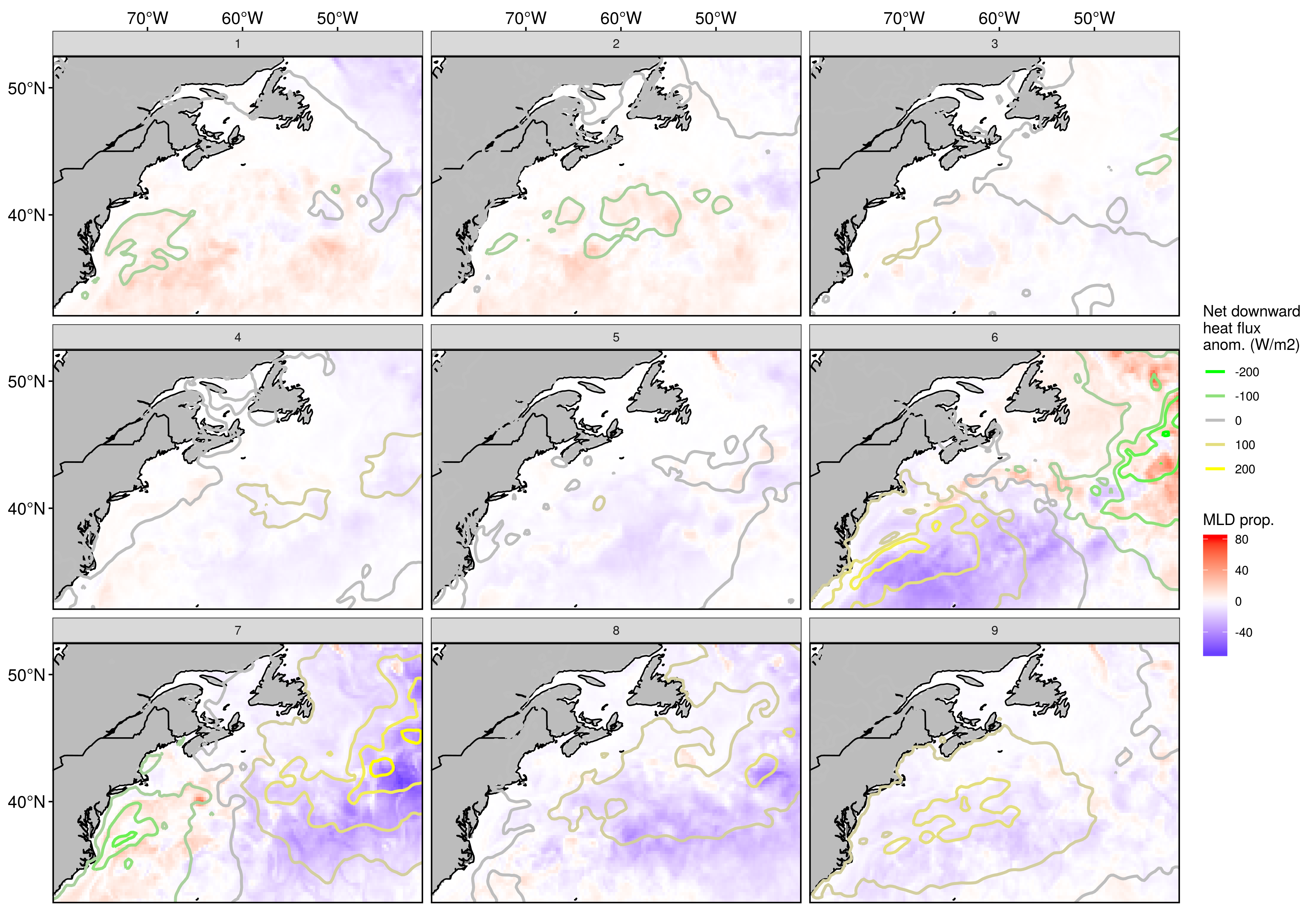
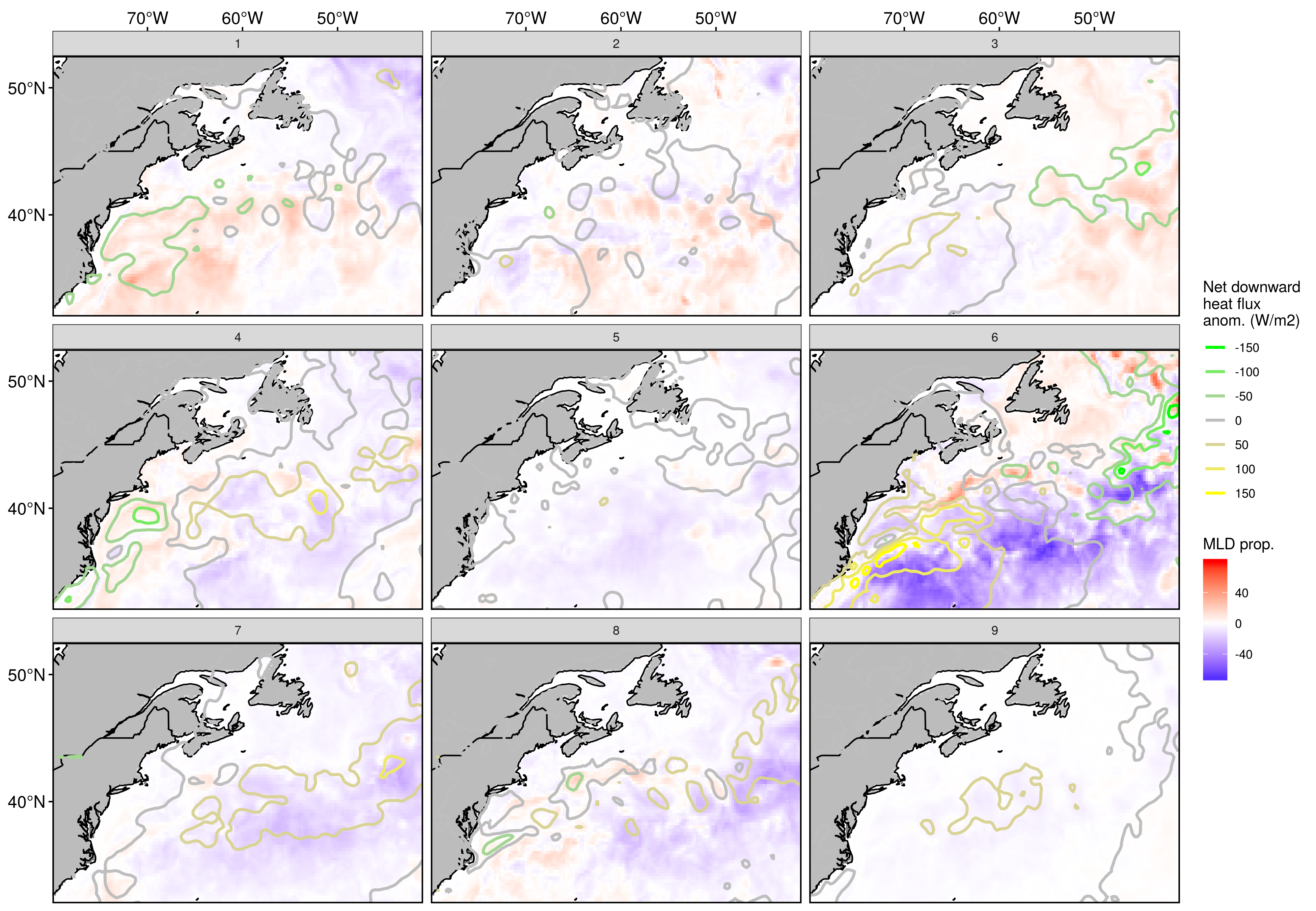
MLD + Net downward heatflux
The top left node (1) shows a decent negative heatflux anomaly over a deep MLD in the GS + AO, while a bit shallow and weakly positive over the LS. This flips over to the opposite as we move diagonally down to the bottom right node (9). Node 7 has a very deep GS with a very strong negative heatflux while showing a shallow AO + GS with a very strong positive heatflux. The opposite of node 7 may be seen in node 6.
Expand here to see past versions of fig_4.png:
| Version | Author | Date |
|---|---|---|
| 9273f18 | robwschlegel | 2019-08-11 |
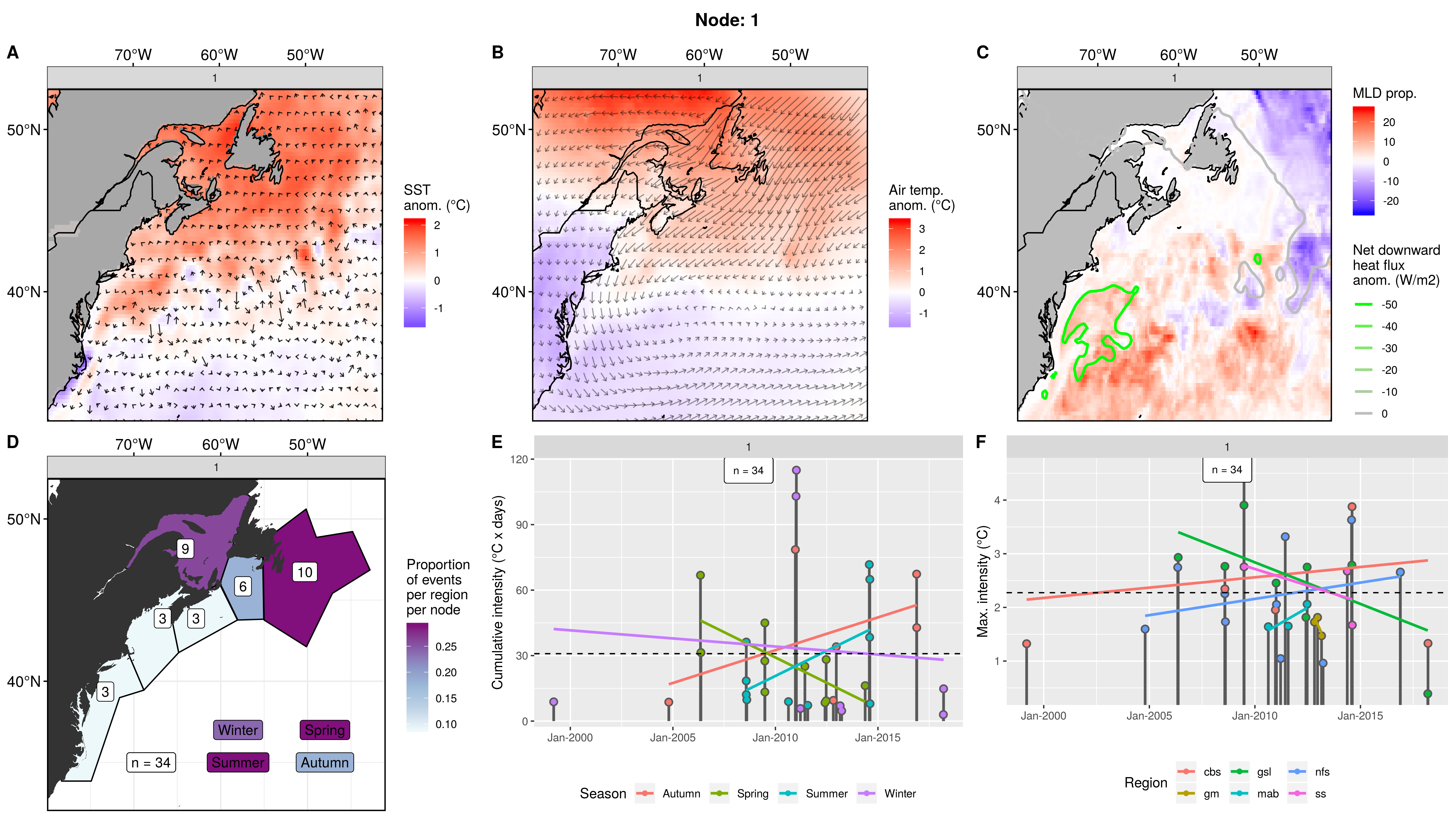
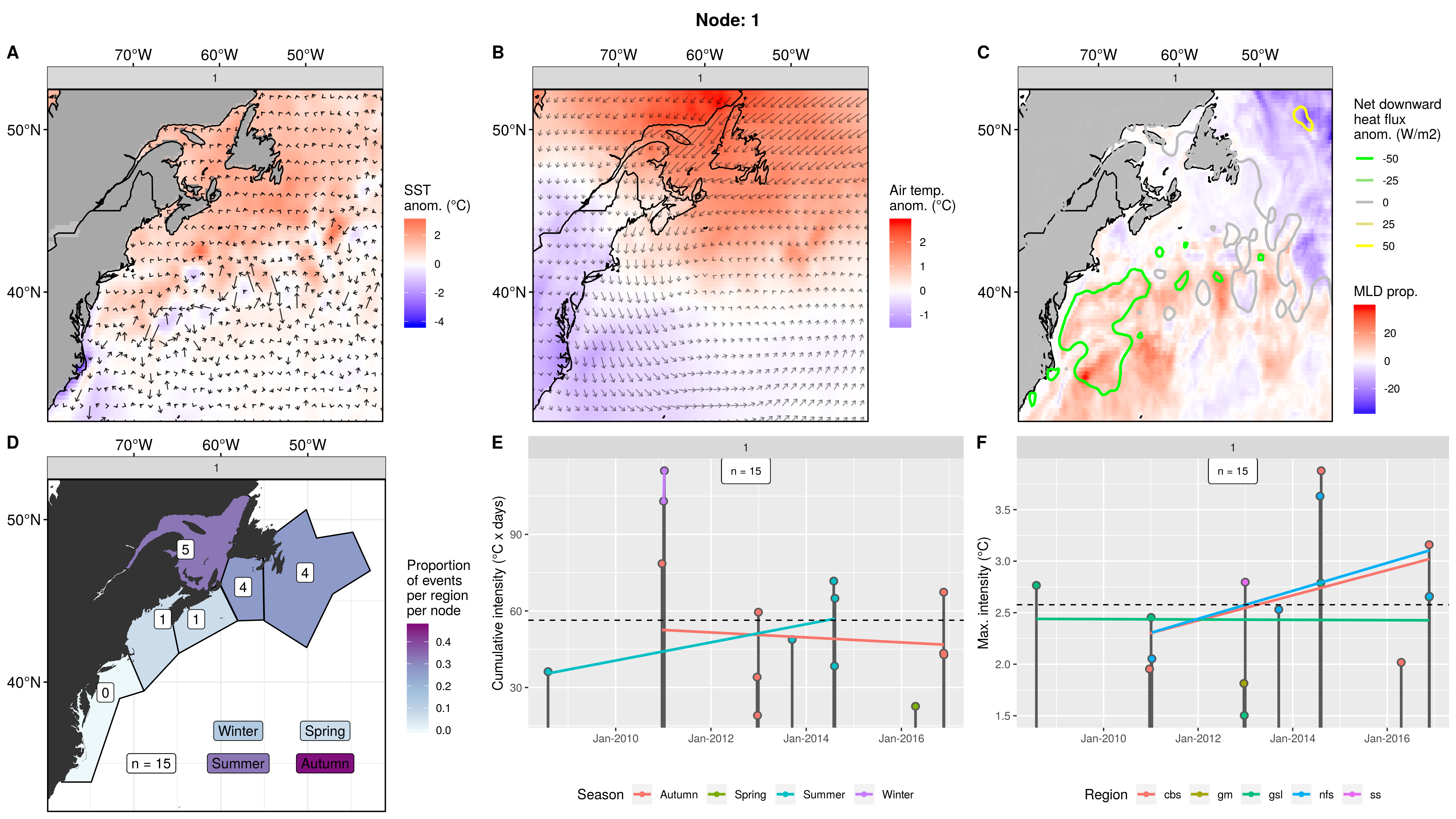
Node 1
This node is mostly nfs and gsl MHWs. With some in the cbs and only 3 each in the other regions. Keep in mind now that because there are only 9 nodes, there are on average ~35 per node. Events here occurred from 1999 - 2017but are clumped up more around the middle of that range. There is a tendency towards spring - summer events, but the autumn events are as large as those, with the winter events being either the smallest or the largest. The average size of these events are small, with many very small events, a few mediums and a couple of large events. There are many small maximum intensities but many of them are large at 3C or greater.
Cold GS and AO SST with some eddy activity. Warm water around the gsl, cbs, and nfs. The wind pattern in this node is wild. Very strong winds from the northeast push very warm wind down onto the gsl region, but this air becomes anomalously cool as it reaches the US. The LS is a bit shallow, but there is no positive heatflux into it. There is a small negative heatflux over the deeper GS and very little negative heatflux over the deeper AO.
This looks like some sort of crazy wind coming from Greenland bringing aseasonally warm air onto the nfs and gsl. This air appears to be somewhat cooler than what would normally be happening over the GS/AO at that time and so doesn’t usually cause events in the more southern coastal regions.
Expand here to see past versions of node_1_panels.png:
| Version | Author | Date |
|---|---|---|
| 9273f18 | robwschlegel | 2019-08-11 |
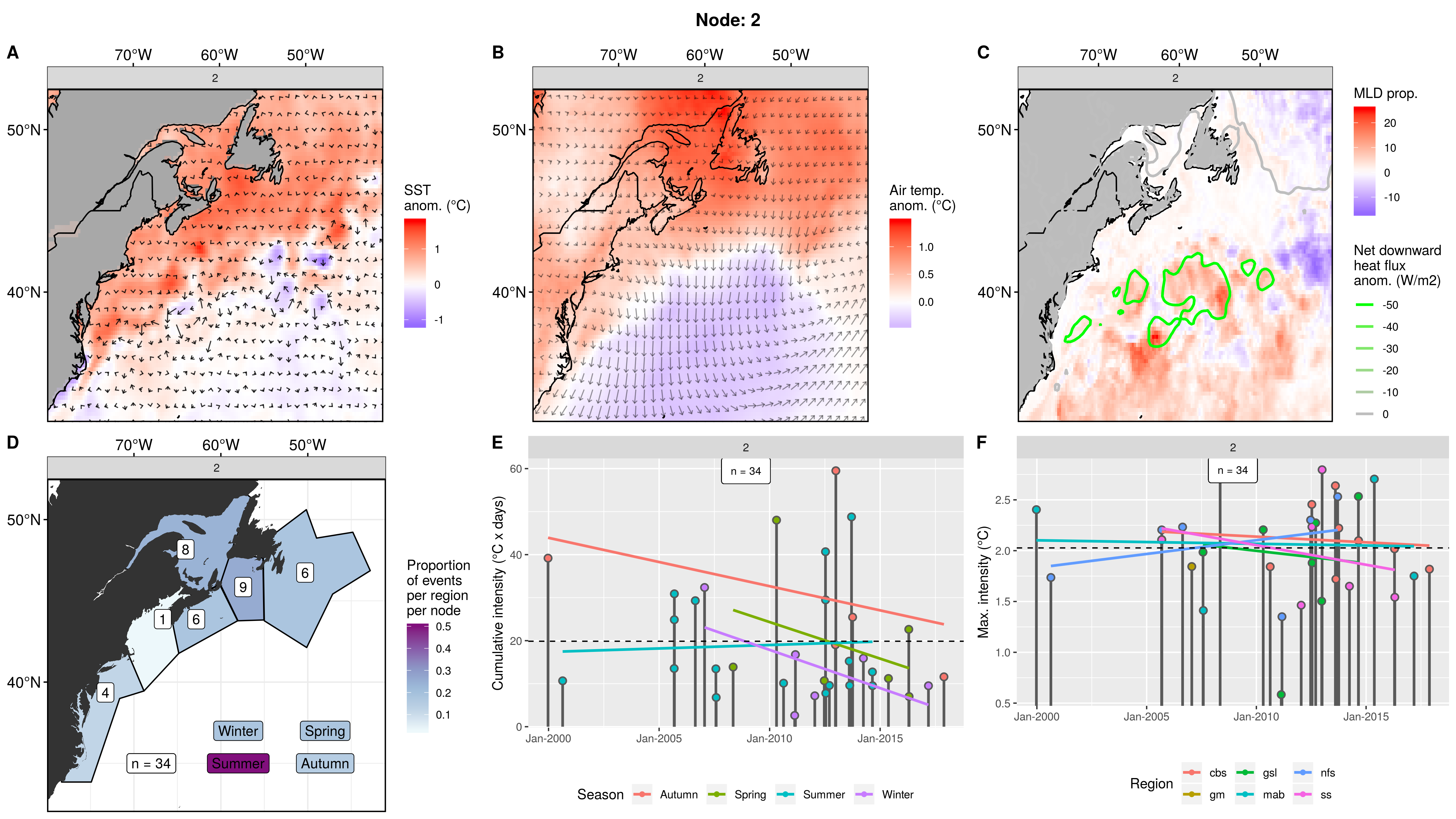
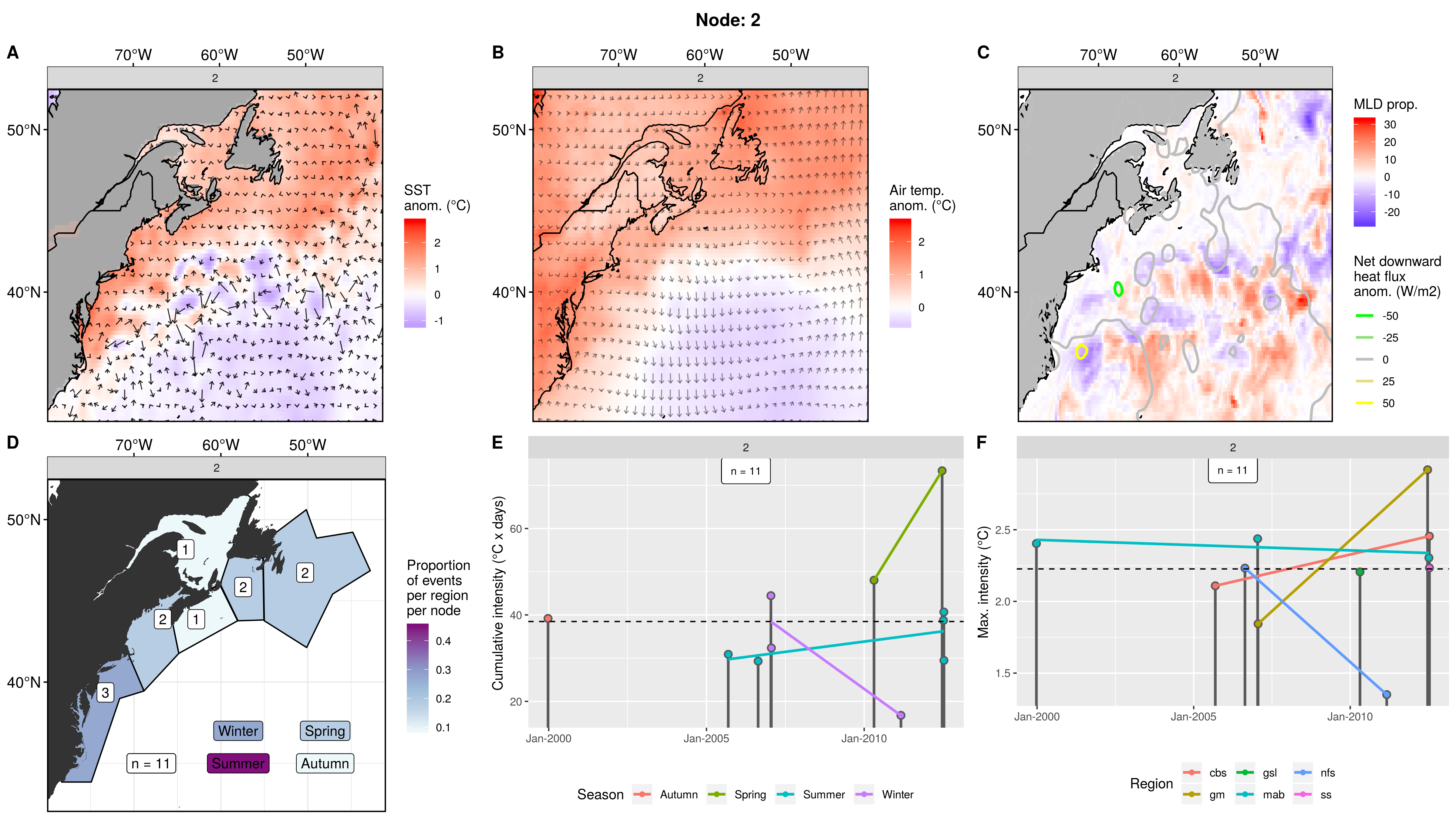
Node 2
Half of the events in this node occurred in the summer and are centralised over the cbs, becoming fewer the further away the regions are. Curiously there is only 1 MHW in the gm. MHWs occurred from 1999 - 2017 and are well distributed with no season appearing to be much larger than the others. The cumulative and max intensities show the normal range for MHWs in the study area.
Not much happening in the GS or AO with some eddy activity. Lukewarm SST anomalies in the other regions. Lukewarm air over CN + US with the warmer anomaly centred to the north of the gsl. Very mild cold anomaly over the AO with the border between warm and cold about where the GS is. At this border the wind anomalies begin to point southward and increase in speed. There is a small cyclone in the left middle of the study area. Most of the study area has a ~10 metre MLD anomaly with a weak negative downward heatflux roughly mirroring the MLD. The MLD over the shelf is very normal and slightly deeper in the LS.
This node shows what is usually aseasonally warm summer air sitting over the northern portion of the study region. As the wind begins to move anomalously southward, especially after crossing the GS, it is no longer anomalously warm.
Expand here to see past versions of node_2_panels.png:
| Version | Author | Date |
|---|---|---|
| 9273f18 | robwschlegel | 2019-08-11 |
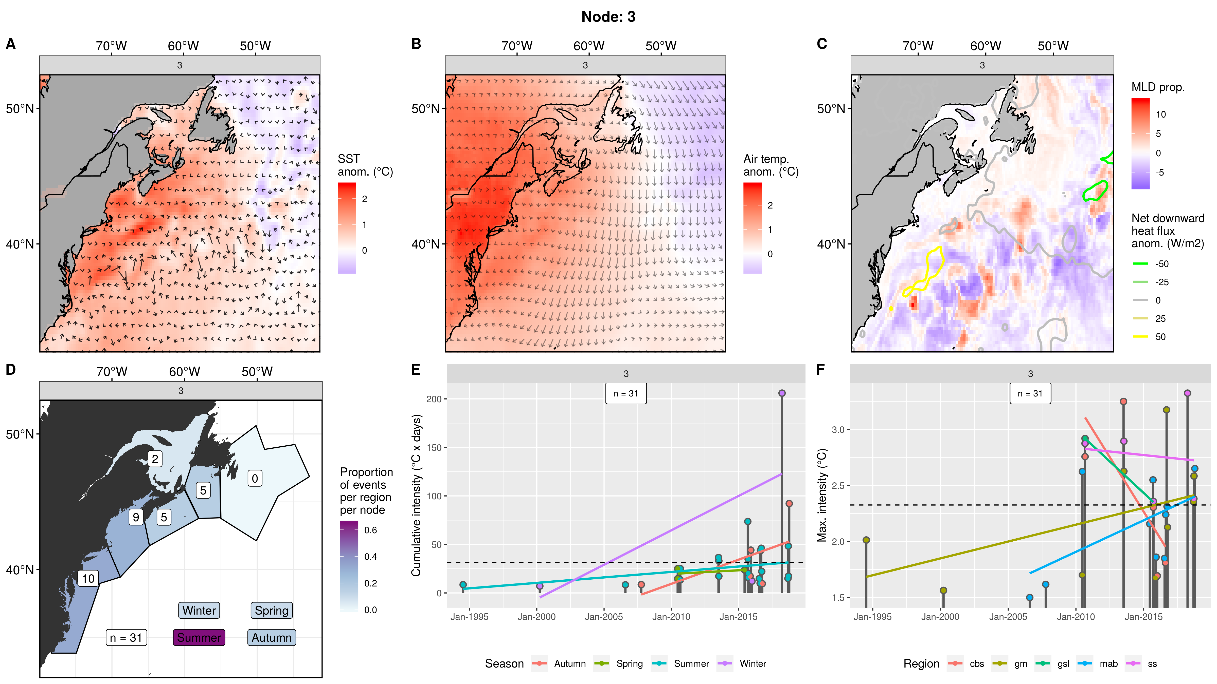
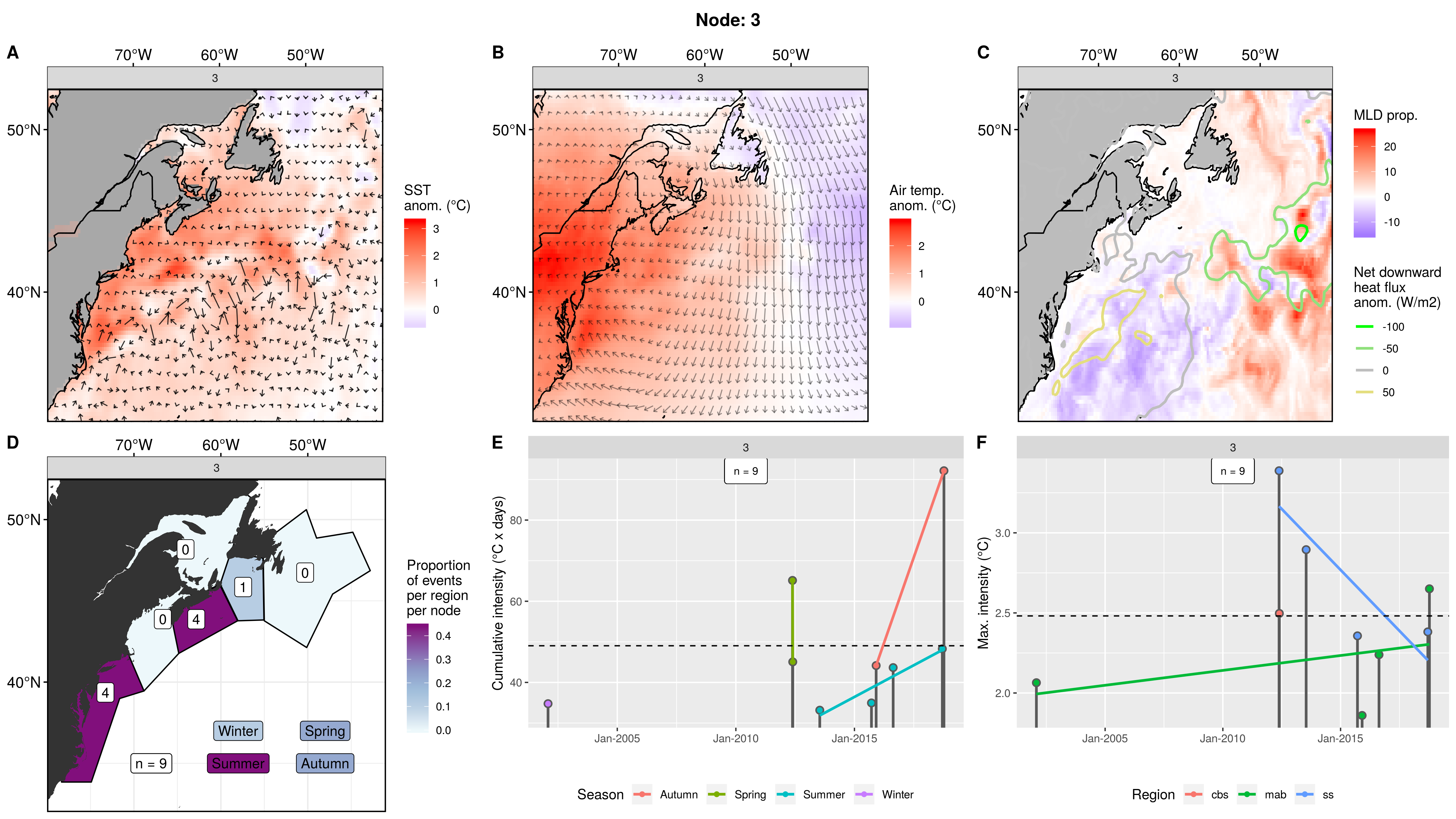
Node 3
More than half of the MHWs in this node are from the summer and are strongly focused on the southern regions, with 10 MHWs counted in the mab and the numbers decreasing from there with only 2 in the gsl and 0 in the nfs. Events occurred here from 1994 - 2017, but didn’t start to occur regularly until 2010. A winter 2017 event here is massive, with the rest of the events showing a more normal range of cumulative intensities. The max intensities in this node are on the high end, especially in the second half of the occurrence of the time series.
A very warm GS and AO, perhaps pushing onto the shelf, with some eddy movement. Mildly cold LS. Weak cold air anomaly over the LS and very warm over the US. Less warm over the GS, AO, and other coastal regions. Anomalous southern wind coming from LS and moving down and out over the AO. No real MLD anomalies to speak of, just eddy cores showing up. There is a weak positive heatflux into the GS and some negative heatflux over the LS/AO meeting area.
The lack of a core for a wind cell, in combination with the very flat MLD anomalies makes me think that this is a large warm body of air being advected either up the coast or from over land that is sitting a rather high air anomaly over the southern coastal regions, but turns away before reaching the nfs, perhaps due to the colder LS.
Expand here to see past versions of node_3_panels.png:
| Version | Author | Date |
|---|---|---|
| 9273f18 | robwschlegel | 2019-08-11 |
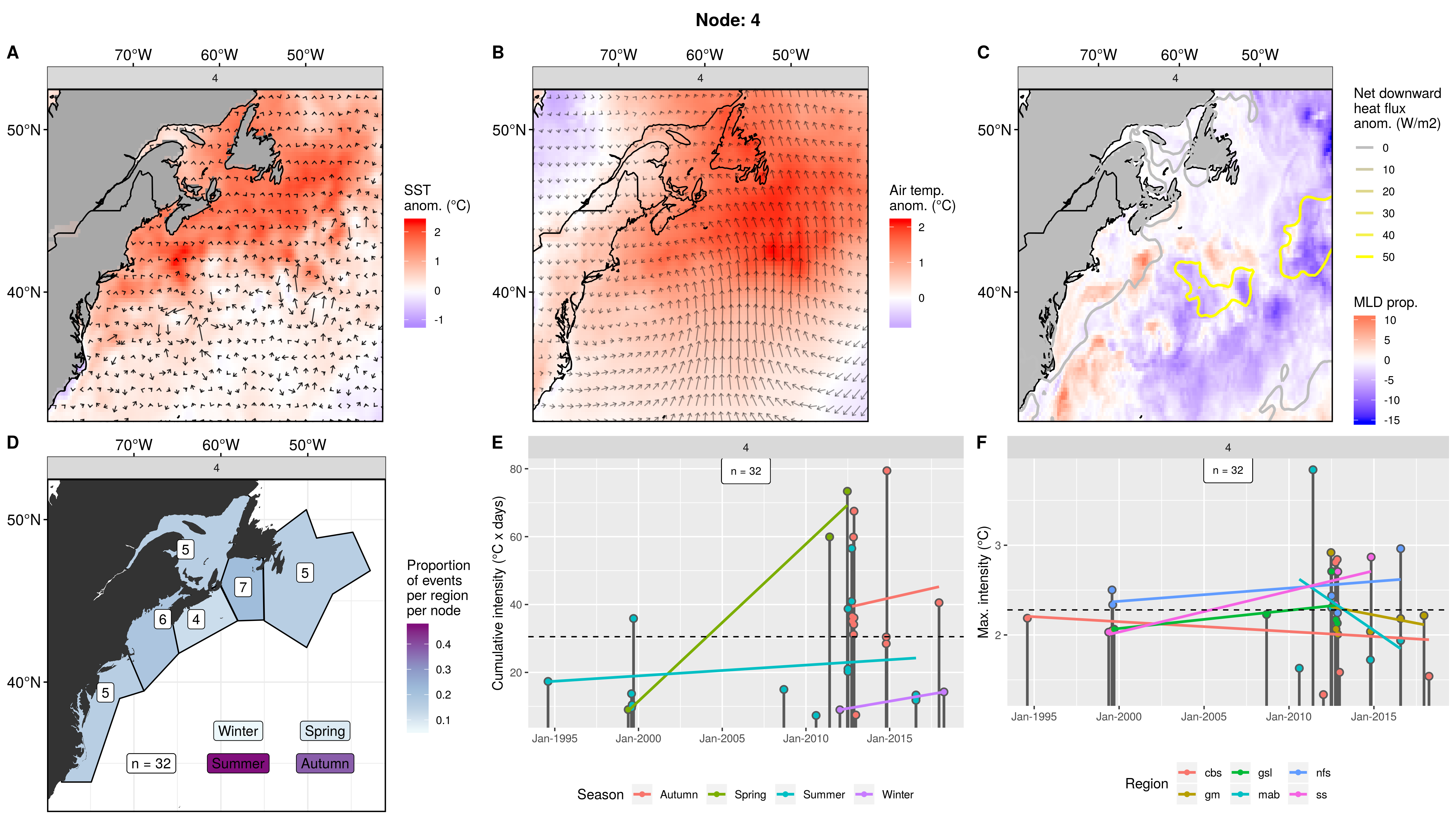
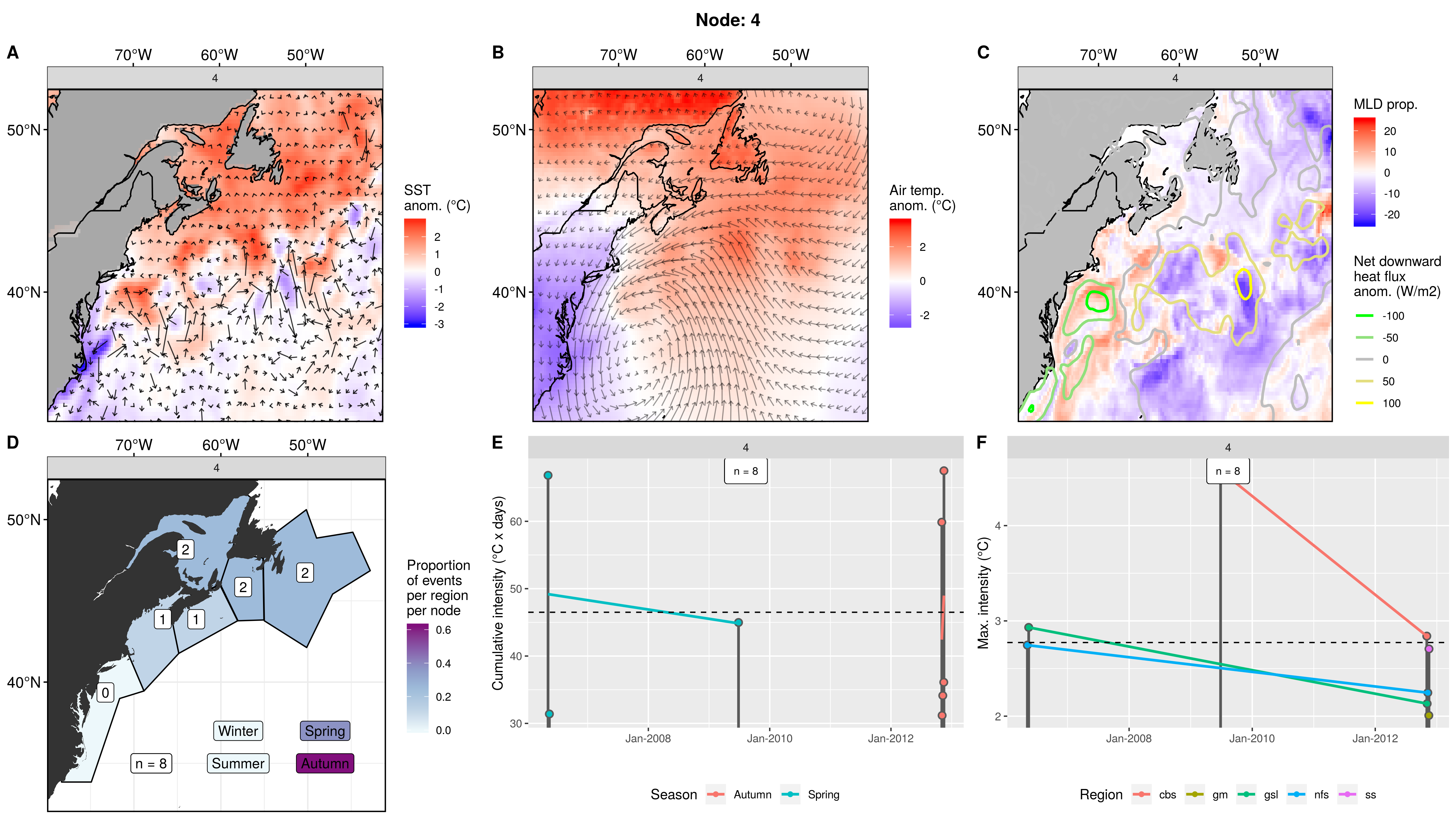
Node 4
The distribution of MHWs by region is very even, with almost all events occurring in summer - autumn. There are only 2 winter and 3 spring events. MHWs occur from 1994 - 2017, with most in the second half. These events are a bit larger on average than the other nodes.
Not much happening in the GS or AO, but warm SST everywhere else. Possibly two opposite rotating cells meeting over the AO pushing warm air up towards the coast. The air over nfs continues northwards while the wind over the other regions looses any anomalous movement. The air over inland CN is slightly cool, which one doesn’t usually see in these results. Either side of the GS is a bit deep, with the rest of the study area being slightly shallow. There is a weak positive heatflux over the shallower regions.
I’m thinking this is some sort of ocean based wind cell that is bringing warm air up from the AO onto the coast. Because it is affecting all regions equally it must be very broad.
Expand here to see past versions of node_4_panels.png:
| Version | Author | Date |
|---|---|---|
| 9273f18 | robwschlegel | 2019-08-11 |
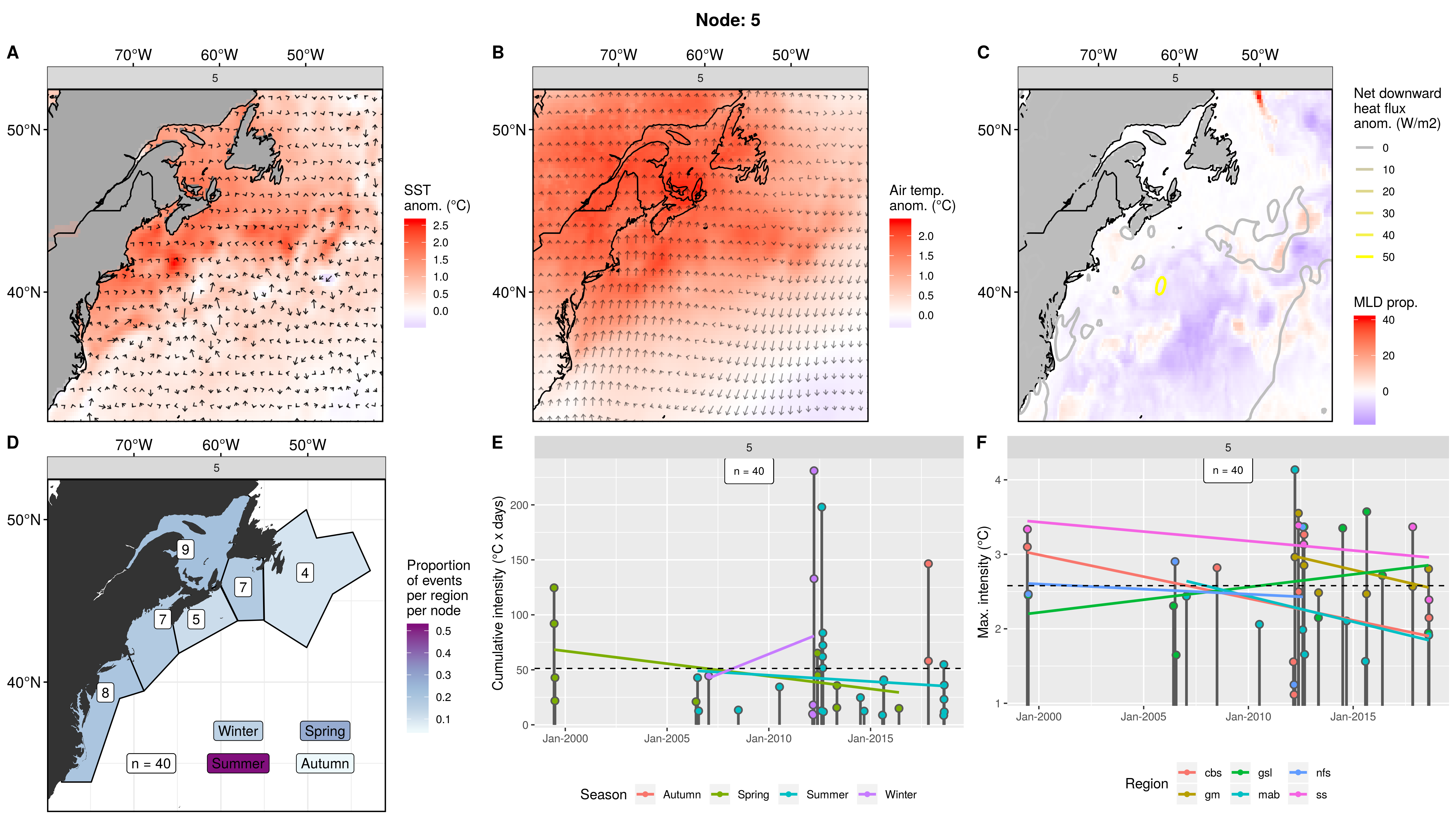
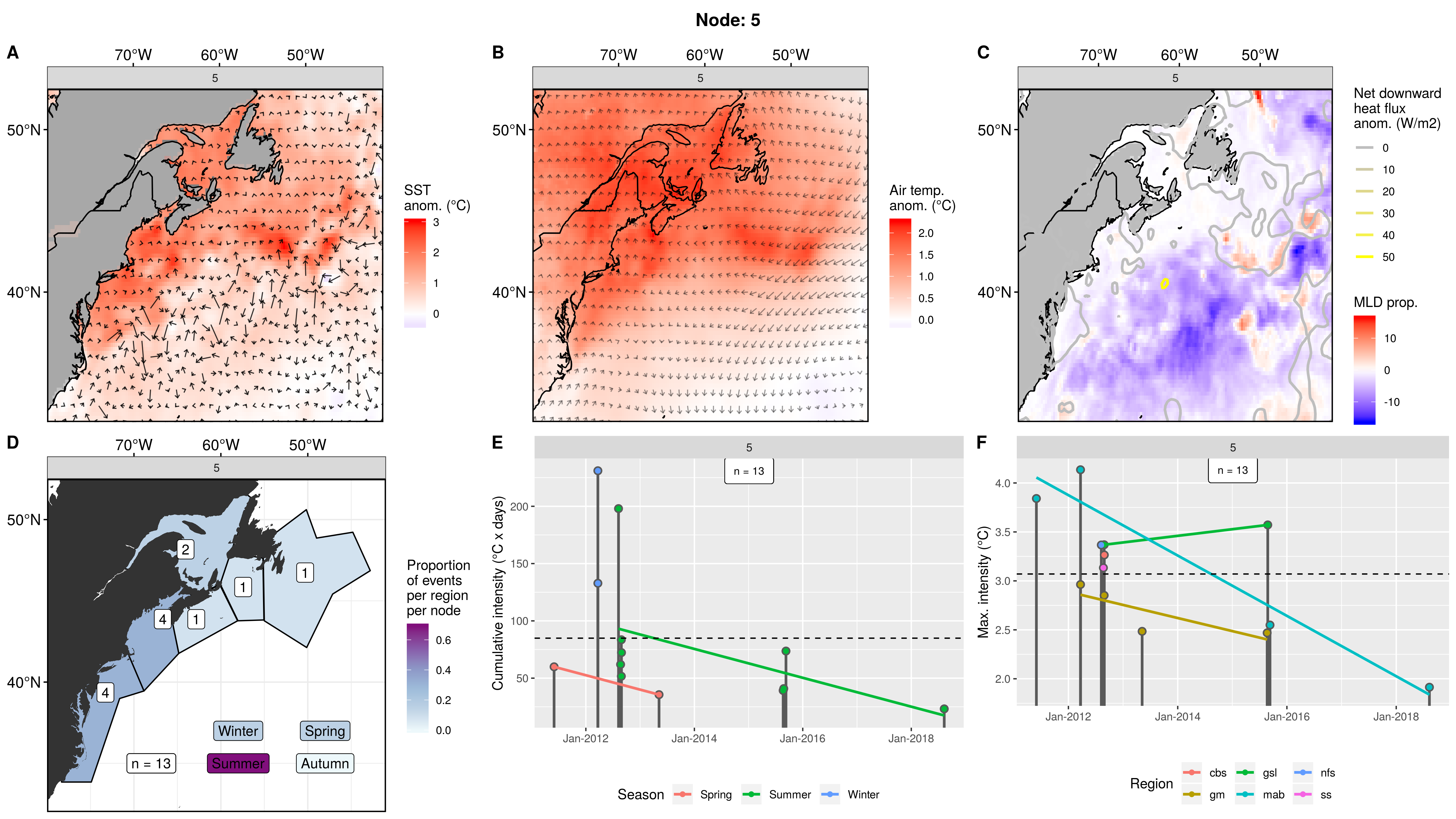
Node 5
The MHWs are pretty evenly spread, with the highest count in the gsl and then the mab, with the nfs having a few less. Over half of the events were in summer and a good amount in spring. Only 2 events occurred in autumn and these were both in 2017. The range of events is mostly from 2006 - 2018, with one pulse of 4 events in the spring of 1999. The smaller events tend to occur by themselves, but the larger events (and some are massive) tend to occur simultaneously across multiple regions. In fact the MHWs in this node are more clumped up than usual. The max intensities are also very high.
Warm SST everywhere, highest to the north of the flow of the GS. Warm air nearly everywhere but highest over the US - CN border + NS. There is a vague anticyclone centred over the AO. The AO and GS are ~10 metres shallower than normal, with a deep tongue of water in the LS. Weak positive heatflux over almost the whole study area, centred over the waters south of the ss.
This looks like some sort of possibly ocean based wind cell that is helping to push warm air up the coast that then sits around the gsl, but for some reason doesn’t really impact nfs as much as the rest of the coastline.
Expand here to see past versions of node_5_panels.png:
| Version | Author | Date |
|---|---|---|
| 9273f18 | robwschlegel | 2019-08-11 |
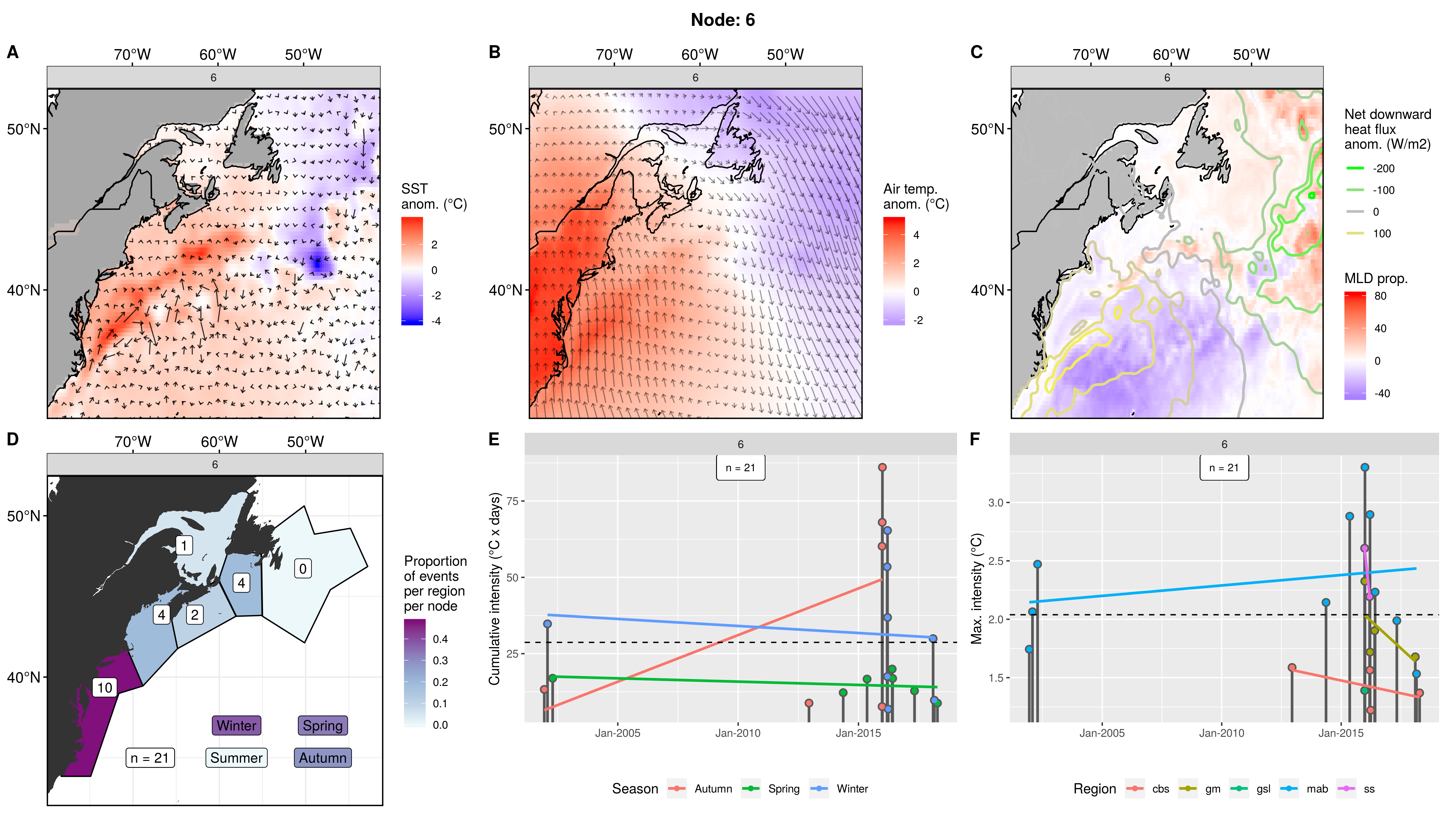
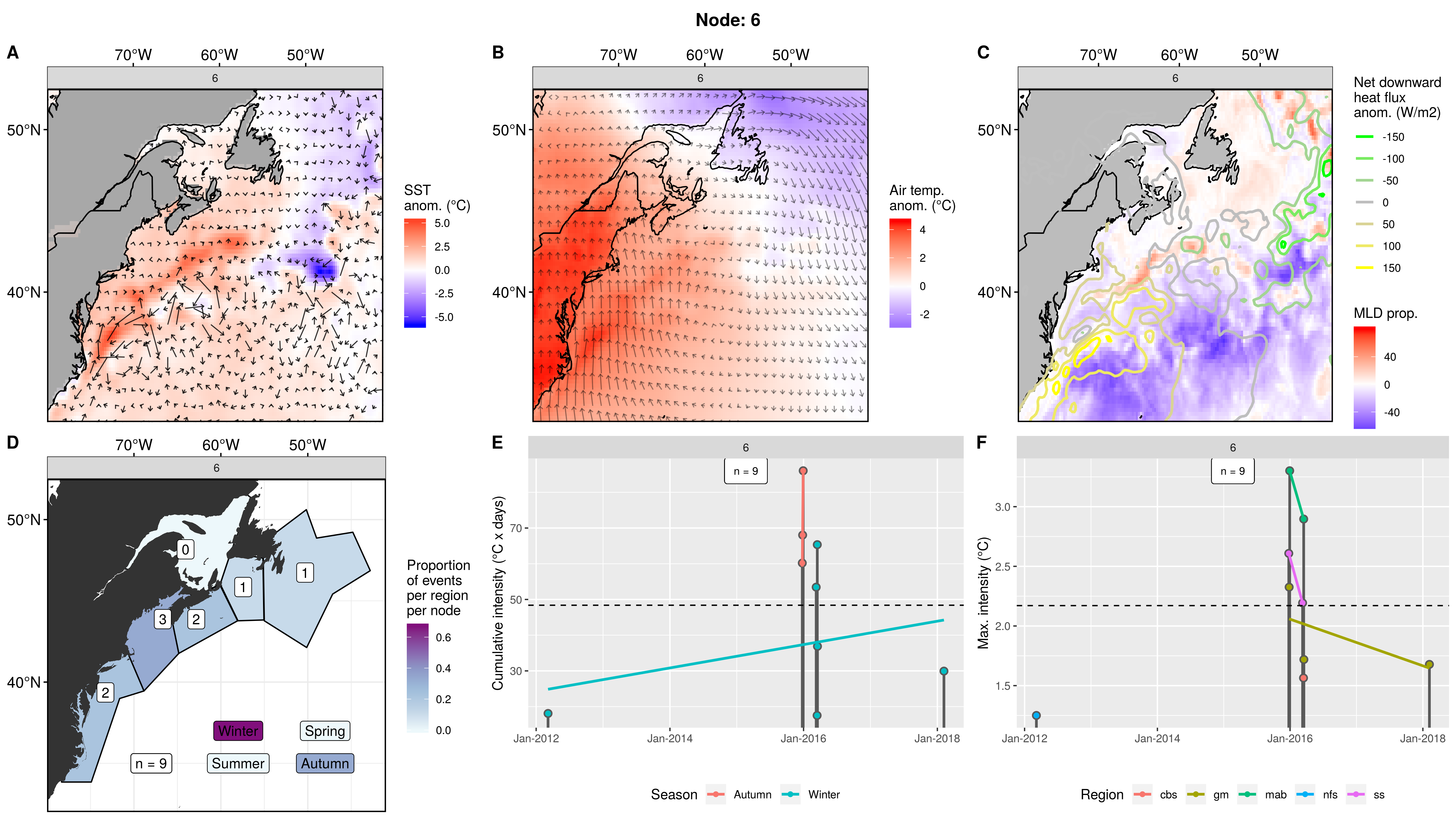
Node 6
Almost entirely mab MHWs with some bleed into the other regions and none in the nfs. Mostly winter MHWs, some in spring or autumn, 0 in summer. Mostly 2013 – 2018 with 3 events in the mab over autumn – spring, 2002 – 2003. There were two decent sized pulses of events in autumn – winter 2016. The max intensities range from low-middle to high.
A very strong warm GS that meets a very cold LS. Massive atmospheric thermal dipole after NS before the gsl. Crazy high air temperature anomaly over US (5C). Warmer air has northward anomaly and colder air has southward anomaly. Very shallow GS and AO with strong positive heatflux while an extremely deep (~40 – 80 metres)LS and eastern AO.
These MHWs are caused by a confluence of a warm fast moving GS bringing warm water closer to the coast and a massive heat anomaly over land that is being advected northward by what may be an anticyclonic storm system, but it looks a little wonky.
Expand here to see past versions of node_6_panels.png:
| Version | Author | Date |
|---|---|---|
| 9273f18 | robwschlegel | 2019-08-11 |
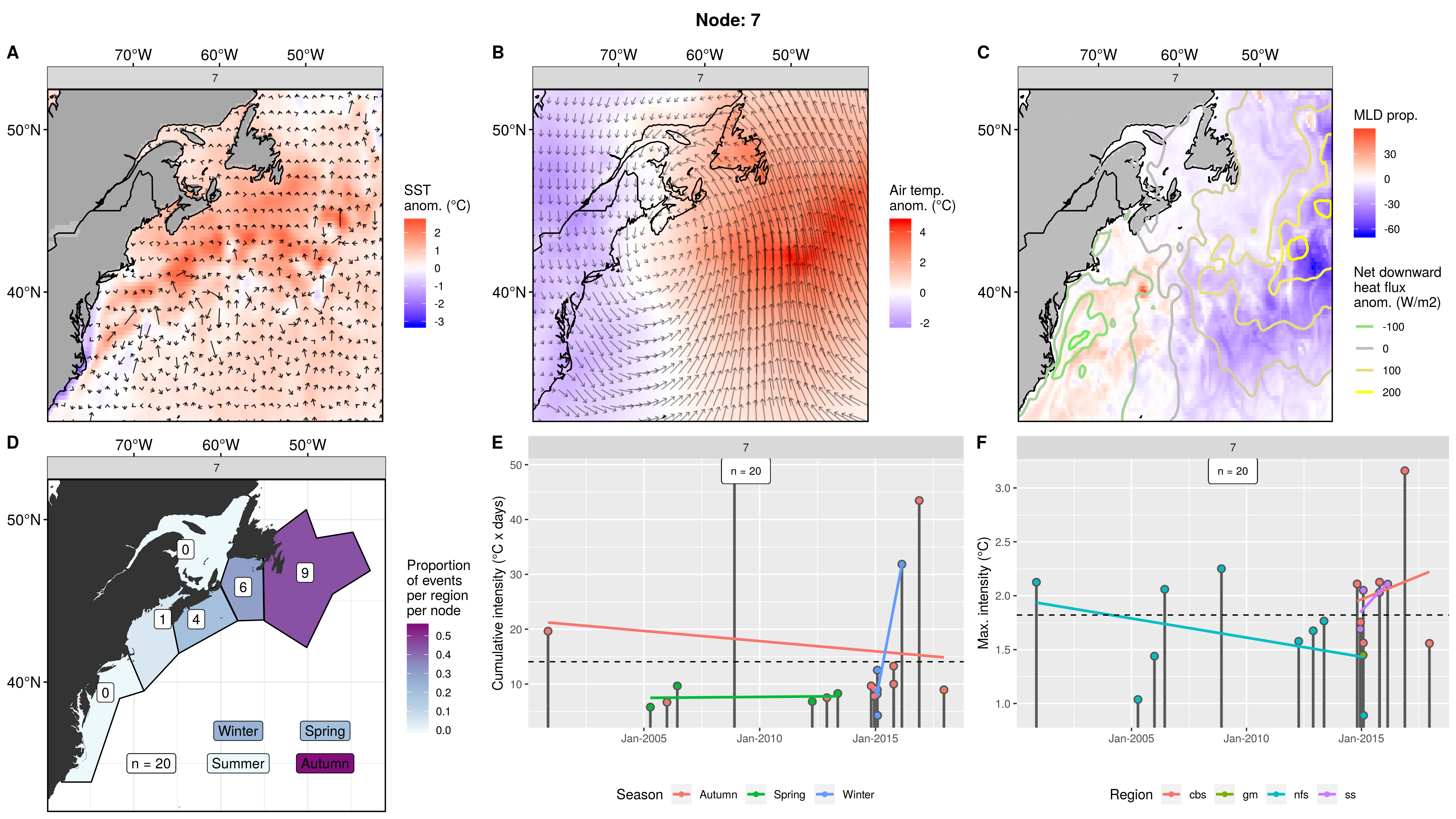
Node 7
Almost half of the MHWs occurred in the nfs, with the next largest in the cbs then ss. Only 1 in the gm and none in the gsl or mab. More than half of the events occurred in the autumn, 4 in spring and winter, and 0 in summer. The MHWs in this node are little tiny ones, with only 3 of the 20 events having cumulative intensities over 30, with the highest near 50. Range is 2002 – 2017, a bit clumped up during the second half. In a very interesting twist, this event only occurred in the nfs region from 2002 – 2014 before we start to see this pattern reaching to the cbs and nfs. A surprisingly clear bit of support for a phenological shift. The maximum intensities of the events are on the higher side on average, with a single event being over 3C.
Very cold GS along the coast (possible upwelling?) but warm SST everywhere else. Warmest SST anomalies on the northern range of the GS as it moves over the AO. Very high air temperature anomaly over the AO/LS that is in the middle of a very strong northwestward wind anomaly. There is a very well defined cyclone centred over the ss that is at the middle of a thermal dipole, with the air anomaly over land being cold. Very shallow LS/AO (-60 metres) with a massive positive heatflux that roughly follows the MLD. Strong negative heatflux out of the deeper GS.
This looks to be a massive autumn storm that moves up from perhaps Mexico, bringing extremely anomalously warm air up with it over the ocean and shoves it onto the nfs while simultaneously pulling cold air down from CN that appears to actually be impacting the temperature of the GS.
Expand here to see past versions of node_7_panels.png:
| Version | Author | Date |
|---|---|---|
| 9273f18 | robwschlegel | 2019-08-11 |
Node 8
MHWs centred around nfs, with many events in cbs and gsl, too. Only 3 events each in the other regions. Relatively even for seasons with a weighting towards winter and away from summer. MHWs occurred from 1999 – 2017, evenly distributed with only a couple of clumps. low-normal range of cumulative intensities and a normal range of max intensities.
Cold GS along coast with some warmer eddies pushing up near the shelf south of ss, everywhere else warm. Very warm air anomaly over Newfoundland, and slightly cold overland near the GS coast. Large anticyclone bringing warm air up over the ocean and across the nfs. Most of the study area is either normal MLD or shallow. This shoaling corresponds with increased strong positive heatflux. The GS is a bit deeper than normal and has almost no heatflux.
This is an any season storm that is bringing warm air up from over the AO and dumping it onto the coast, mostly on the nfs and surrounding regions.
Expand here to see past versions of node_8_panels.png:
| Version | Author | Date |
|---|---|---|
| 9273f18 | robwschlegel | 2019-08-11 |
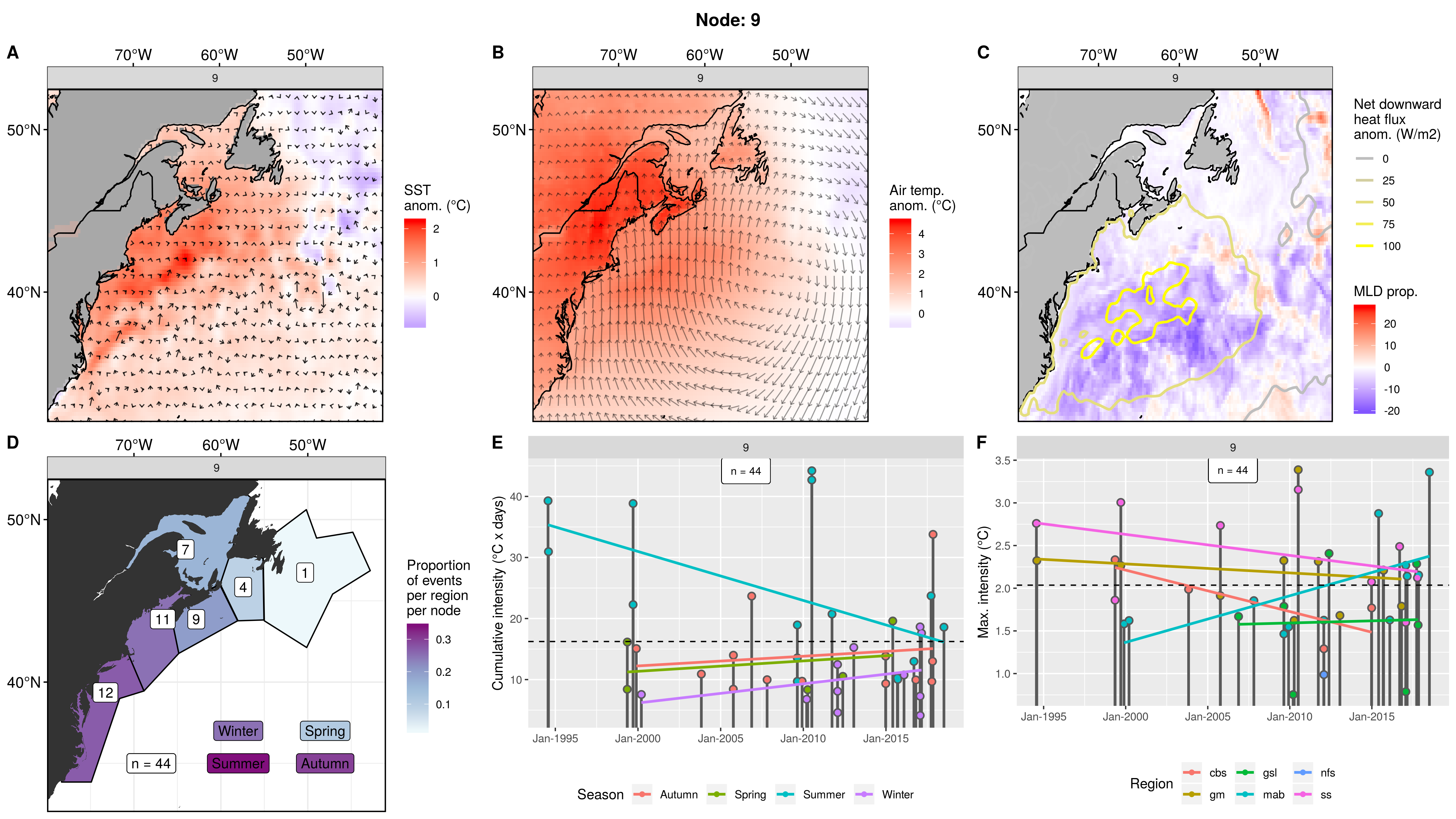
Node 9
MHWs centred on the mab, radiating out less from there with only 1 MHW in the nfs. The are mostly summer then autumn events, with some in winter and only 5 in spring. This node has a very large count of MHWs at 44. These events are very small on average, with the largest events occurring in summer, but only with cumulative intensities of 40. The max intensities are a bit high on average. Events occur here from 1994 – 2018.
The waters above the GS are warm with the SST anomaly in the AO only mildly warm while the LS is only a little cool. Massive anticyclone sitting just southwest of the LS. Enormous hot air anomaly over US - CN border + NS but almost no wind anomaly over land. Large positive heatflux centred over the GS after it has moved away from the coast. There is a ~-10 – -20 MLD anomaly for most of the GS and AO with some deeper waters under the centre of the anticyclone.
This node appears to show a large, mostly summer – autumn, storm that is bringing hot air up onto the continent and then leaving it there, but it doesn’t quite reach over to the nfs. It may also be driving the GS to be a bit stronger.
Expand here to see past versions of node_9_panels.png:
| Version | Author | Date |
|---|---|---|
| 9273f18 | robwschlegel | 2019-08-11 |
SOM experiment: Default, no events under 14 days, 3x3 nodes
In this SOM experiment we removed all events shorter than 14 days (2 weeks). This is a bit of a thumb suck but is based on the idea that thermal stress probably only starts to become a problem for most organisms after 2 weeks. This is of course very debatable. The other reason for setting the 14 day duration limit is that it filters our MHWs down from 289 to 103. The thinking behind this is that ~100 synoptic states is a nicer number for a 3x3 SOM, and hypothetically it will produce crisper results.
Node summary table
The table below contains a concise summary of the nodes following Table 4 in Oliver et al. (2018). The following sub-sections provide more in-depth explanations.
| Node | Region | Season | MHW Properties | Conditions |
|---|---|---|---|---|
| 1 |
Season + region
With this reduced run of MHWs we see the same pattern as before that the left-hand column has predominantly nfs focused MHWs and no mab MHWs. Moving to the right however the pattern of increasing mab MHWs and decreasing nfs MHWs does not hold up great, but it is vaguely there. We also see that the highest proportion of gsl MHWs occur in the top left node (1) and decrease as we move diagonally away. There doesn’t appear to be too much of a pattern in seasonal occurrence across the nodes, but there are many nodes with a high proportion of events from only one season. Much more so than with the larger MHW sample sizes above. I think that we don’t see many nfs MHWs because they tend to be smaller and were probably screen out more so than for the other regions.
Expand here to see past versions of fig_5.png:
| Version | Author | Date |
|---|---|---|
| 9273f18 | robwschlegel | 2019-08-11 |
SST + U + V
The nodes here are similar to the 3x3 nodes above in that we see a cooler LS in the right-hand column that tends to warm up as we move left. The AO is cooler in the top row and warms as we move down. The GS is colder in the left-hand column and warms as we move right. All panels show marked eddy activity, more so than the previous two SOM experiments. This is almost certainly because there are fewer synoptic states per node so the minor details like eddies don’t get smoothed out as much.
Expand here to see past versions of fig_2.png:
| Version | Author | Date |
|---|---|---|
| 9273f18 | robwschlegel | 2019-08-11 |
Air temp + U + V
Many of these nodes are nearly identical to the 3x3 SOM experiment. Only nodes 4, 7, and 8 appear somewhat different. This may be due to splitting or joining of other nodes. The LS tends to be cooler in the right-hand column and warms to the left. The air over the AO is cooler in the top left node (1) and warms diagonally away. The middle two nodes (5, 8) are warm everywhere. We see anticyclones in the right-hand column and cyclones in the left. The middle nodes 2 and 5 show somewhat southward moving anomalies, while node 8 shows northward movement. Node 7 shows perhaps a convergence of two opposite spinning cells.
Expand here to see past versions of fig_3.png:
| Version | Author | Date |
|---|---|---|
| 9273f18 | robwschlegel | 2019-08-11 |
MLD + Net downward heatflux
The similarities between these nodes and the default 3x3 results persist, but the MLD anomalies for nodes 1 + 2 are a bit different around the GS as it moves across the study area. The general pattern across the nodes is that the left-hand column has a positive MLD anomaly over the GS with a negative heatflux, while showing a negative MLD anomaly over the LS and AO with a positive heatflux term. This pattern is muted in the middle column, and reversed in the right-hand column.Node 8 looks like it would better be swapped with node 7, so there must be some other more important variable at play here. Node 9 in particular shows very little anomalies for either MLD or heatflux.
Expand here to see past versions of fig_4.png:
| Version | Author | Date |
|---|---|---|
| 9273f18 | robwschlegel | 2019-08-11 |
Node 1
This node is tied with node 9 for the highest count of MHWs at 15, meaning this is a common pattern for lengthy/large MHWs. The MHWs take place largely in the gsl, nfs, and cbs, with only 1 event each in the ss + gm and 0 MHWs in the mab. About half the events occurred in autumn, with spill-over into summer, only 2 winter events and 1 spring event. These events occurred from 2008 – 2016 in 7 distinct pulses, 4 of which triggered MHWs in 2 – 3 regions at once. The cumulative intensity and max intensities are on the higher end.
The GS is a bit cold here with the SST of the AO being unremarkable, the rest of the coastal regions are warmer. The atmosphere shows a massive thermal dipole cyclone situated to the south of the cbs with winds pushing anomalously warm air down from northern CA over the nfs + gsl + cbs but the warm anomaly looses power as it reaches NS. The GS and much of the AO are anomalously deep with a weak negative heatflux. The LS shows the opposite while the coastal waters from the gm and up are just barely shallower than normal with a minor negative heatflux.
This is clearly some sort of storm that is somehow pulling air south along the coastline, but the temperature of that air stops being anomalous once it passes the cbs.
Expand here to see past versions of node_1_panels.png:
| Version | Author | Date |
|---|---|---|
| 9273f18 | robwschlegel | 2019-08-11 |
Node 2
This node shows a good spread of affected regions, with the weighting towards the two ends (mab + nfs), which is a bit odd. About half of these were summer events, with winter , spring, and autumn being decreasingly present in that order. MHWs occurred from 1999 – 2012. There were 7 occurrences of this event for a total of 11 MHWs. The events here are on the low side of average with only one being slightly noteworthy.
A cold AO with a lot of cold core eddies. Warm coastal regions but the cold cores are pushing towards the ss. Warm air anomaly over land and the coastal waters but cold over the AO. Anomalous southward air movement along the border between the warm and cold air that turns back up northwards in a vaguely cyclonic motion. The MLD anomaly is all over the place and appears to be dominated by the eddy field. There is some positive heatflux over the partially shallower GS but also negative heatflux just downstream from that. This is the messiest MLD node I’ve seen in this study.
This one is a bit odd. I’m thinking that because of all of the cold core eddy activity that the GS is being forced funny somewhere outside of the study area while we are also getting some sort of cold air cell that is causing even more mixing over the AO. This is all going on while the air over the continent is warm and wanting to just sit on the coastal waters.
Expand here to see past versions of node_2_panels.png:
| Version | Author | Date |
|---|---|---|
| 9273f18 | robwschlegel | 2019-08-11 |
Node 3
MHWs being triggered in the mab + ss, with 1 in the cbs. These are half summer events with spill-over into spring + autumn and 1 winter event. 2 of the 7 occurrence of this events triggered MHWs in two regions. The main range of MHWs in this node is 2012 – 2018, with the one winter event in 2002. These are medium sized events with higher range of max intensities.
A warm AO and very warm fast moving turbulent shelf pushing GS. LS is a mix of warm and cold. Warm air anomaly over US with fast southward wind anomaly in cold air over LS/AO. This turns northward cyclonically offshore of the mab. Shallow MLD over GS with positive heatflux. LS and AO have mostly positive MLD anomaly and negative heatflux.
This appears to be a GS driven MHW pattern. It looks like it is transporting warm water and air northwards, which is causing the MHWs in the mab and ss. But this doesn’t explain the presence of the strong southward wind anomaly over the LS.
Expand here to see past versions of node_3_panels.png:
| Version | Author | Date |
|---|---|---|
| 9273f18 | robwschlegel | 2019-08-11 |
Node 4
Mostly northern regions showing up as MHWs in this node, fading to 0 events in the mab. This pattern occurred only 3 times from 2006 – 2012, causing 8 MHWs. The first two occurrences were in spring. The third and last occurrence was in autumn and caused MHWs in 5 regions at once. The cumulative intensities are normal, but the max intensities are on the high end, with one being over 5C!
The GS is incredibly cool here with massive eddy activity. Some of which appear to be pushing warm water towards the shelf. The coastal regions from the gm up become increasingly warmer. There is an enormous cyclonic anomaly sitting offshore of the mab, drawing cold air down over the US and the gm + mab. There is also a little anticyclone above the nfs that appears to be helping to push warm air of over the shelf there. The GS is maybe pushing up onto the coast south of Cape Cod, judging by the anomalous positive MLD signal there in conjunction with a strong negative heatflux term. Most of the rest of the AO and LS are shallow with positive heatflux.
This appears to be a pretty rare spring or autumn storm that is pulling air up from the south and dumping it onto the coast mostly north of NS. The proximity of the storm to the coastline is such that it is drawing anomalously cool air down over the southern regions.
Expand here to see past versions of node_4_panels.png:
| Version | Author | Date |
|---|---|---|
| 9273f18 | robwschlegel | 2019-08-11 |
Node 5
Mostly MHWs in the southern regions, weakening in the northern regions but everywhere saw at least 1 MHW. Almost all summer events with just 2 in spring and winter. 6 occurrences of this pattern led to the 13 MHWs, with one pulse in summer 2013 causing MHWs in 5 regions at once. The cumulative intensity of the events is massive and most of the max intensities are as well. This is by far the node with the largest MHWs in the entire study. MHWs from 2011 to 2018.
The GS is perhaps moving a bit faster and is more turbulent with shelf waters being very warm. In fact the SST for the entire study area is warm. The air anomaly is warm everywhere, too, with a focus over the coastal regions centred on the gm. There is little anomalous wind movement over the study regions. Perhaps just enough to be holding the warm air in place over the shelf. Most of the study region shows a negative MLD anomaly and minor positive heatflux.
This node looks like the GS may be transporting warm water northwards that then interacts with a lazy atmosphere to allow the whole heat blanket to just sit on the coast. Judging from the size of the MHWs this does not look like a case of advection, rather that things are sitting sedentary for long periods of time.
Expand here to see past versions of node_5_panels.png:
| Version | Author | Date |
|---|---|---|
| 9273f18 | robwschlegel | 2019-08-11 |
Node 6
No MHWs in the gsl and a roughly even distribution otherwise, focused on the gm. These are almost always winter events with one pulse in autumn. MHWs occurred from 2012 – 2018 in 4 pulses. The middle two pulses caused 3 and 4 MHWs respectively. The cumulative and max intensities are on the higher end. Interestingly, the order of the max intensity of the MHWs in each region during the two large pulses are the same. The solo 2012 occurrence of this pattern caused only 1 small MHW in the nfs and so I would guess this isn’t actually matching this pattern well, but was just clumped in here by the SOM.
A very fast moving GS coming up along the coast bringing crazy hot water up against the shelf. This is then offset by it meeting a cold LS and appearing to then deflect anomalously south, judging by the eddy field vectors. Very hot air anomaly overland with strong anomalous northward winds. The wind turns east and then south in an anticyclonic pattern upon reaching the gsl and cooling. The GS itself is not anomalously shallow, but the waters to either side of it are. The main thrust of the GS is covered by a focused large positive heatflux anomaly. The LS and Grand Banks are anomalously deep in most places with the LS having a strong negative heatflux.
This is another chicken vs. egg situation where it is not clear if the strong GS is driving warm water northwards, which then causes a warm air anomaly, or if the air anomaly is already there and acts to supercharge the GS. Either way, we see a strong positive heatflux from the atmosphere into the GS which is then transporting warm water against the shelf waters.
Expand here to see past versions of node_6_panels.png:
| Version | Author | Date |
|---|---|---|
| 9273f18 | robwschlegel | 2019-08-11 |
Node 7
These MHWs are centred around the cbs and decrease in count from there, with 0 in the mab. Mostly autumn and summer MHWs with two in spring and one in winter. Occurred from 1999 – 2015 in 6 pulses causing 12 events. Medium intensities.
Overall warm SST, with the waters over the cbs + nfs the warmest. Cold air overland with high anomaly over the nfs. Large anticyclone located to the east of the study area that is bringing warm air up and over the nfs. Mostly negative MLD anomalies with correspondingly strong positive heatflux.
This appears to be a summer/autumn storm that is tracking in from over the AO onto the nfs during a time when the air over the continent is colder than usual.
Expand here to see past versions of node_7_panels.png:
| Version | Author | Date |
|---|---|---|
| 9273f18 | robwschlegel | 2019-08-11 |
Node 8
MHWs centered over the ss and becoming less frequent from there. The occurrence of this pattern is 2014 – 2018, with one small winter nfs MHW in 1999. There are some massive MHWs in this node. There is one small winter nfs MHW in 1999.
This node is very similar to node 7, but with a cool LS and warm air over the continent. The track of the storm appears to be over-land, too. The warmer cores within the GS have a negative heatflux anomaly while most of the study area is shallow with a small positive heatflux.
This is a funny pattern in that it appears that the GS is causing these MHWs, but it meanders out away from the coast for a bit, missing the mab, and then, perhaps to the strong warm wind anomaly, tries to turn back into the shelf. This explains the pattern of observed MHWs by region being centred around the ss but with no events in the gsl.
Expand here to see past versions of node_8_panels.png:
| Version | Author | Date |
|---|---|---|
| 9273f18 | robwschlegel | 2019-08-11 |
Node 9
MHWs centred over the gm and reducing from there. Mostly summer events with some spill-over into spring and autumn. Ranged evenly from 1994 to 2018. One pulse in spring/summer of 1999 caused some large MHWs. The max intensities are on the high end.
Unremarkable GS with cool LS and warm shelf waters. Very clear anticyclonic storm moving north over the AO pulling up warm air over the coastal waters south of NS. Minor negative MLD in most of study area with a small positive heatflux centred within the storms eye.
Summer storm bringing warm air north, especially onto NS itself. [I wonder if this is what caused the heatwave in September 2018.]
Expand here to see past versions of node_9_panels.png:
| Version | Author | Date |
|---|---|---|
| 9273f18 | robwschlegel | 2019-08-11 |
References
Oliver, E. C., Lago, V., Hobday, A. J., Holbrook, N. J., Ling, S. D., and Mundy, C. N. (2018). Marine heatwaves off eastern tasmania: Trends, interannual variability, and predictability. Progress in oceanography 161, 116–130.
Richaud, B., Kwon, Y.-O., Joyce, T. M., Fratantoni, P. S., and Lentz, S. J. (2016). Surface and bottom temperature and salinity climatology along the continental shelf off the canadian and us east coasts. Continental Shelf Research 124, 165–181.
Session information
R version 3.6.1 (2019-07-05)
Platform: x86_64-pc-linux-gnu (64-bit)
Running under: Ubuntu 16.04.5 LTS

Matrix products: default
BLAS:   /usr/lib/openblas-base/libblas.so.3
LAPACK: /usr/lib/libopenblasp-r0.2.18.so

locale:
 [1] LC_CTYPE=en_CA.UTF-8       LC_NUMERIC=C
 [3] LC_TIME=en_CA.UTF-8        LC_COLLATE=en_CA.UTF-8
 [5] LC_MONETARY=en_CA.UTF-8    LC_MESSAGES=en_CA.UTF-8
 [7] LC_PAPER=en_CA.UTF-8       LC_NAME=C
 [9] LC_ADDRESS=C               LC_TELEPHONE=C
[11] LC_MEASUREMENT=en_CA.UTF-8 LC_IDENTIFICATION=C

attached base packages:
[1] stats     graphics  grDevices utils     datasets  methods   base

loaded via a namespace (and not attached):
 [1] workflowr_1.1.1   Rcpp_0.12.18      digest_0.6.16
 [4] rprojroot_1.3-2   R.methodsS3_1.7.1 backports_1.1.2
 [7] git2r_0.23.0      magrittr_1.5      evaluate_0.11
[10] highr_0.7         stringi_1.2.4     whisker_0.3-2
[13] R.oo_1.22.0       R.utils_2.7.0     rmarkdown_1.10
[16] tools_3.6.1       stringr_1.3.1     yaml_2.2.0
[19] compiler_3.6.1    htmltools_0.3.6   knitr_1.20
This reproducible R Markdown analysis was created with workflowr 1.1.1