Preparing the data
Robert Schlegel
2020-02-25
Last updated: 2020-02-26
Checks: 7 0
Knit directory: MHWflux/
This reproducible R Markdown analysis was created with workflowr (version 1.6.0). The Checks tab describes the reproducibility checks that were applied when the results were created. The Past versions tab lists the development history.
Great! Since the R Markdown file has been committed to the Git repository, you know the exact version of the code that produced these results.
Great job! The global environment was empty. Objects defined in the global environment can affect the analysis in your R Markdown file in unknown ways. For reproduciblity it’s best to always run the code in an empty environment.
The command set.seed(20200117) was run prior to running the code in the R Markdown file. Setting a seed ensures that any results that rely on randomness, e.g. subsampling or permutations, are reproducible.
Great job! Recording the operating system, R version, and package versions is critical for reproducibility.
Nice! There were no cached chunks for this analysis, so you can be confident that you successfully produced the results during this run.
Great job! Using relative paths to the files within your workflowr project makes it easier to run your code on other machines.
Great! You are using Git for version control. Tracking code development and connecting the code version to the results is critical for reproducibility. The version displayed above was the version of the Git repository at the time these results were generated.
Note that you need to be careful to ensure that all relevant files for the analysis have been committed to Git prior to generating the results (you can use wflow_publish or wflow_git_commit). workflowr only checks the R Markdown file, but you know if there are other scripts or data files that it depends on. Below is the status of the Git repository when the results were generated:
Ignored files:
    Ignored:    .Rhistory
    Ignored:    .Rproj.user/

Unstaged changes:
    Modified:   code/functions.R
    Modified:   code/workflow.R
Note that any generated files, e.g. HTML, png, CSS, etc., are not included in this status report because it is ok for generated content to have uncommitted changes.
These are the previous versions of the R Markdown and HTML files. If you’ve configured a remote Git repository (see ?wflow_git_remote), click on the hyperlinks in the table below to view them.
| File | Version | Author | Date | Message |
|---|---|---|---|---|
| Rmd | 891e53a | robwschlegel | 2020-02-26 | Published site for first time. |
| Rmd | 1be0a1e | robwschlegel | 2020-02-26 | Completed the data prep for the project |
| Rmd | bcd165b | robwschlegel | 2020-02-26 | Writing |
| Rmd | 29883d6 | robwschlegel | 2020-02-26 | Calculated the MHWs from GLORYS data. Am now wrestling with the pipeline for ERA5 loading. |
| Rmd | c4343c0 | robwschlegel | 2020-02-26 | Pushing quite a few changes |
| Rmd | 80324fe | robwschlegel | 2020-02-25 | Adding the foundational content to the site |
Introduction
Much of the code in this vignette is taken entirely or partially from the study area prep, the MHW prep, and the gridded data prep vignettes from the drivers of MHWs in the NW Atlantic project. Because this process has already been established we are going to put it all together in this one vignette in a more streamlined manner.
All of the libraries and functions used in this vignette, and the project more broadly may be found here.
# get everything up and running in one go
source("code/functions.R")
library(SDMTools) # For finding points within polygons
Study area
A reminder of what the study area looks like. It has been cut into 6 regions, adapted from work by Richaud et al. (2016).
frame_base +
  geom_polygon(data = NWA_coords, alpha = 0.7, size = 2,
               aes(fill = region, colour = region)) +
  geom_polygon(data = map_base, aes(group = group))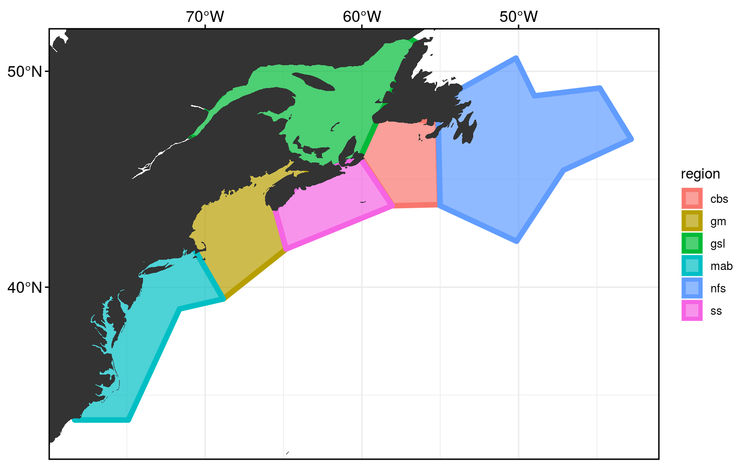
Pixels per region
In this study it was decided to use the higher resolution 1/12th degree GLORYS data. This means we will need to re-calculate which pixels fall within which region so we can later determine how to create our average SST time series per region as well as the other averaged heat flux term time series.
# Load one GLORYS file to extract the lon/lat coords
GLORYS_files <- dir("../data/GLORYS", full.names = T, pattern = "MHWflux")
GLORYS_grid <- tidync(GLORYS_files[1]) %>%
  hyper_tibble() %>%
  dplyr::rename(lon = longitude, lat = latitude) %>%
  dplyr::select(lon, lat) %>%
  unique()

# Load one ERA5 file to get the lon/lat coords
ERA5_files <- dir("../../oliver/data/ERA/ERA5/LWR", full.names = T, pattern = "ERA5")
ERA5_grid <- tidync(ERA5_files[1]) %>%
  hyper_filter(latitude = dplyr::between(latitude, min(NWA_coords$lat), max(NWA_coords$lat)),
               longitude = dplyr::between(longitude, min(NWA_coords$lon)+360, max(NWA_coords$lon)+360),
               time = index == 1) %>%
  hyper_tibble() %>%
  dplyr::rename(lon = longitude, lat = latitude) %>%
  dplyr::select(lon, lat) %>%
  unique() %>%
  mutate(lon = lon-360)

# Function for finding and cleaning up points within a given region polygon
pnts_in_region <- function(region_in, product_grid){
  region_sub <- NWA_coords %>%
    filter(region == region_in)
  coords_in <- pnt.in.poly(pnts = product_grid[,c("lon", "lat")], poly.pnts = region_sub[,c("lon", "lat")]) %>%
    filter(pip == 1) %>%
    dplyr::select(-pip) %>%
    mutate(region = region_in)
  return(coords_in)
}

# Run the function
GLORYS_regions <- plyr::ldply(unique(NWA_coords$region), pnts_in_region,
                              .parallel = T, product_grid = GLORYS_grid)
saveRDS(GLORYS_regions, "data/GLORYS_regions.Rda")
ERA5_regions <- plyr::ldply(unique(NWA_coords$region), pnts_in_region,
                            .parallel = T, product_grid = ERA5_grid)
saveRDS(ERA5_regions, "data/ERA5_regions.Rda")
GLORYS_regions <- readRDS("data/GLORYS_regions.Rda")
ERA5_regions <- readRDS("data/ERA5_regions.Rda")
# Combine for visual
both_regions <- rbind(GLORYS_regions, ERA5_regions) %>%
mutate(product = c(rep("GLORYS", nrow(GLORYS_regions)),
rep("ERA5", nrow(ERA5_regions))))
# Visualise to ensure success
ggplot(NWA_coords, aes(x = lon, y = lat)) +
# geom_polygon(aes(fill = region), alpha = 0.2) +
geom_point(data = both_regions, aes(colour = region)) +
geom_polygon(data = map_base, aes(group = group), show.legend = F) +
coord_cartesian(xlim = NWA_corners[1:2],
ylim = NWA_corners[3:4]) +
labs(x = NULL, y = NULL) +
facet_wrap(~product)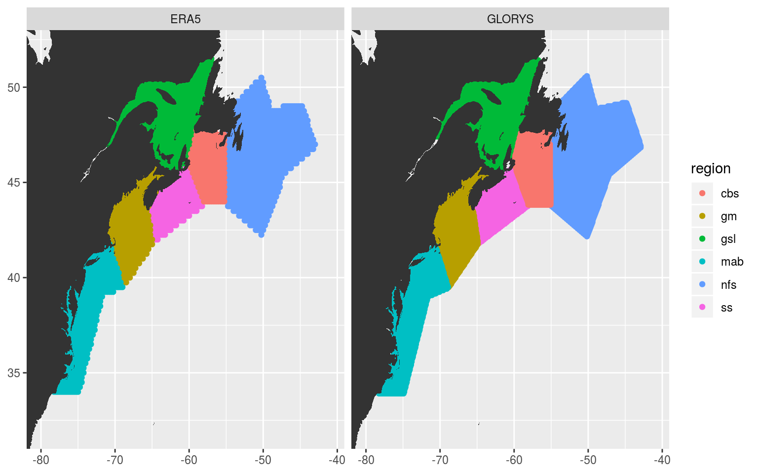
Average time series per region
With our pixels per region sorted we may now go about creating the average time series for each region from the GLORYS and ERA5 data. First we will load a brick of the data constrained roughly to the study area into memory before assigning the correct pixels to their regions. Once the pixels are assigned we will summarise them into one mean time series per variable per region. These mean time series are what the rest of the analyses will depend on.
The code for loading and processing the GLORYS data.
# Set number of cores
  # NB: This is very RAM heavy, be carfeul with core use
doParallel::registerDoParallel(cores = 25)

# The GLORYS file location
GLORYS_files <- dir("../data/GLORYS", full.names = T, pattern = "MHWflux")
system.time(
GLORYS_all_ts <- load_all_GLORYS_region(GLORYS_files) %>%
  dplyr::arrange(region, t)
) # 187 seconds on 25 cores
saveRDS(GLORYS_all_ts, "data/GLORYS_all_ts.Rda")
The code for the ERA5 data. NB: The ERA5 data are on an hourly 0.25x0.25 spatiotemporal grid. This loading process constrains them to a daily 0.25x0.25 grid.
# See the code/workflow script for the code used for ERA5 data prep
# There is too much code to run from an RMarkdown document
MHWs per region
We will be using the SST value from GLORYS for calculating the MHWs and will use the standard Hobday definition with a base period of 1993-01-01 to 2018-12-25. We are using an eneven length year as the data do not quite extend to the end of December. It was decided that the increased accuracy of the climatology from the 2018 year outweighed the negative consideration of having a clim period that excludes a few days of winter.
# Load the data
GLORYS_all_ts <- readRDS("data/GLORYS_all_ts.Rda")

# Calculate the MHWs
GLORYS_region_MHW <- GLORYS_all_ts %>%
  dplyr::select(region:temp) %>%
  group_by(region) %>%
  nest() %>%
  mutate(clims = map(data, ts2clm,
                     climatologyPeriod = c("1993-01-01", "2018-12-25")),
         events = map(clims, detect_event),
         cats = map(events, category, S = FALSE)) %>%
  select(-data, -clims)

# Save
saveRDS(GLORYS_region_MHW, "data/GLORYS_region_MHW.Rda")
Clims + anoms per variable
The analyses to come are going to be performed on anomaly values, not the original time series. In order to calculate the anomalies we are first going to need the climatologies for each variable. We will use the Hobday definition of climatology creation and then subtract the expected climatology from the observed values. We are again using the 1993-01-01 to 2018-12-25 base period for these calculations to ensure consistency throughout the project.
# Load the data
GLORYS_all_ts <- readRDS("data/GLORYS_all_ts.Rda")
ERA5_all_ts <- readRDS("data/ERA5_all_ts.Rda")
ALL_ts <- left_join(ERA5_all_ts, GLORYS_all_ts, by = c("region", "t"))

# Calculate GLORYS clims and anoms
ALL_anom <- ALL_ts %>%
  pivot_longer(temp:t2m, names_to = "var", values_to = "val") %>%
  group_by(region, var) %>%
  nest() %>%
  mutate(clims = map(data, ts2clm, y = val, roundClm = 6,
                     climatologyPeriod = c("1993-01-01", "2018-12-25"))) %>%
  dplyr::select(-data) %>%
  unnest(cols = clims) %>%
  mutate(anom = val-seas)

# Save
ALL_anom <- saveRDS(ALL_anom, "data/ALL_anom.Rda")
And that’s all there is to it. In the next vignette we will take the periods of time over whiche MHWs occurred per region and pair those up with the GLORYS and ERA5 data. This will be used to investigate which drivers are best related to the onset and decline of MHWs.
References
Richaud, B., Kwon, Y.-O., Joyce, T. M., Fratantoni, P. S., and Lentz, S. J. (2016). Surface and bottom temperature and salinity climatology along the continental shelf off the canadian and us east coasts. Continental Shelf Research 124, 165–181.
sessionInfo()R version 3.6.2 (2019-12-12)
Platform: x86_64-pc-linux-gnu (64-bit)
Running under: Ubuntu 16.04.6 LTS
Matrix products: default
BLAS: /usr/lib/openblas-base/libblas.so.3
LAPACK: /usr/lib/libopenblasp-r0.2.18.so
locale:
[1] LC_CTYPE=en_CA.UTF-8 LC_NUMERIC=C
[3] LC_TIME=en_CA.UTF-8 LC_COLLATE=en_CA.UTF-8
[5] LC_MONETARY=en_CA.UTF-8 LC_MESSAGES=en_CA.UTF-8
[7] LC_PAPER=en_CA.UTF-8 LC_NAME=C
[9] LC_ADDRESS=C LC_TELEPHONE=C
[11] LC_MEASUREMENT=en_CA.UTF-8 LC_IDENTIFICATION=C
attached base packages:
[1] stats graphics grDevices utils datasets methods base
other attached packages:
[1] SDMTools_1.1-221 tidync_0.2.3 heatwaveR_0.4.2.9001
[4] lubridate_1.7.4 forcats_0.4.0 stringr_1.4.0
[7] dplyr_0.8.4 purrr_0.3.3 readr_1.3.1
[10] tidyr_1.0.2 tibble_2.1.3 ggplot2_3.2.1
[13] tidyverse_1.3.0
loaded via a namespace (and not attached):
[1] httr_1.4.1 jsonlite_1.6.1 viridisLite_0.3.0 foreach_1.4.4
[5] R.utils_2.7.0 modelr_0.1.5 assertthat_0.2.1 cellranger_1.1.0
[9] yaml_2.2.1 pillar_1.4.3 backports_1.1.5 lattice_0.20-35
[13] glue_1.3.1 digest_0.6.23 promises_1.1.0 rvest_0.3.5
[17] colorspace_1.4-1 htmltools_0.4.0 httpuv_1.5.2 R.oo_1.22.0
[21] pkgconfig_2.0.3 broom_0.5.3 haven_2.2.0 scales_1.1.0
[25] whisker_0.4 later_1.0.0 git2r_0.26.1 farver_2.0.3
[29] generics_0.0.2 withr_2.1.2 lazyeval_0.2.2 cli_2.0.1
[33] magrittr_1.5 crayon_1.3.4 readxl_1.3.1 evaluate_0.14
[37] R.methodsS3_1.7.1 fs_1.3.1 ncdf4_1.17 fansi_0.4.1
[41] doParallel_1.0.15 nlme_3.1-137 xml2_1.2.2 tools_3.6.2
[45] data.table_1.12.8 hms_0.5.3 lifecycle_0.1.0 plotly_4.9.1
[49] munsell_0.5.0 reprex_0.3.0 compiler_3.6.2 RNetCDF_2.1-1
[53] rlang_0.4.4 grid_3.6.2 iterators_1.0.10 rstudioapi_0.10
[57] htmlwidgets_1.5.1 labeling_0.3 rmarkdown_2.0 gtable_0.3.0
[61] codetools_0.2-15 DBI_1.0.0 R6_2.4.1 ncmeta_0.2.0
[65] knitr_1.27 workflowr_1.6.0 rprojroot_1.3-2 stringi_1.4.5
[69] parallel_3.6.2 Rcpp_1.0.3 vctrs_0.2.2 dbplyr_1.4.2
[73] tidyselect_1.0.0 xfun_0.12