NAFLD patient cohort by Hoang et al.
Last updated: 2020-12-23
Checks: 7 0
Knit directory: meta-liver/
This reproducible R Markdown analysis was created with workflowr (version 1.6.2). The Checks tab describes the reproducibility checks that were applied when the results were created. The Past versions tab lists the development history.
Great! Since the R Markdown file has been committed to the Git repository, you know the exact version of the code that produced these results.
Great job! The global environment was empty. Objects defined in the global environment can affect the analysis in your R Markdown file in unknown ways. For reproduciblity it’s best to always run the code in an empty environment.
The command set.seed(20201218) was run prior to running the code in the R Markdown file. Setting a seed ensures that any results that rely on randomness, e.g. subsampling or permutations, are reproducible.
Great job! Recording the operating system, R version, and package versions is critical for reproducibility.
Nice! There were no cached chunks for this analysis, so you can be confident that you successfully produced the results during this run.
Great job! Using relative paths to the files within your workflowr project makes it easier to run your code on other machines.
Great! You are using Git for version control. Tracking code development and connecting the code version to the results is critical for reproducibility.
The results in this page were generated with repository version d4f78fa. See the Past versions tab to see a history of the changes made to the R Markdown and HTML files.
Note that you need to be careful to ensure that all relevant files for the analysis have been committed to Git prior to generating the results (you can use wflow_publish or wflow_git_commit). workflowr only checks the R Markdown file, but you know if there are other scripts or data files that it depends on. Below is the status of the Git repository when the results were generated:
Ignored files:
    Ignored:    .DS_Store
    Ignored:    .Rhistory
    Ignored:    .Rproj.user/
    Ignored:    analysis/human-diehl-nafld_cache/
    Ignored:    analysis/human-hampe13-nash_cache/
    Ignored:    analysis/human-hampe14-misc_cache/
    Ignored:    analysis/human-ramnath-fibrosis_cache/
    Ignored:    analysis/meta-chronic-vs-acute_cache/
    Ignored:    analysis/meta-mouse-vs-human_cache/
    Ignored:    analysis/mouse-acute-apap_cache/
    Ignored:    analysis/mouse-acute-bdl_cache/
    Ignored:    analysis/mouse-acute-ccl4_cache/
    Ignored:    analysis/mouse-acute-lps_cache/
    Ignored:    analysis/mouse-acute-ph_cache/
    Ignored:    analysis/mouse-acute-tunicamycin_cache/
    Ignored:    analysis/mouse-chronic-ccl4_cache/
    Ignored:    analysis/plot-acute-apap_cache/
    Ignored:    analysis/plot-acute-bdl_cache/
    Ignored:    analysis/plot-acute-ccl4_cache/
    Ignored:    analysis/plot-acute-ph_cache/
    Ignored:    analysis/plot-chronic-ccl4_cache/
    Ignored:    analysis/plot-chronic-vs-acute_cache/
    Ignored:    analysis/plot-precision-recall_cache/
    Ignored:    analysis/plot-study-overview_cache/
    Ignored:    code/.DS_Store
    Ignored:    code/README.html
    Ignored:    data/.DS_Store
    Ignored:    data/README.html
    Ignored:    data/annotation/
    Ignored:    data/human-diehl-nafld/
    Ignored:    data/human-hampe13-nash/
    Ignored:    data/human-hampe14-misc/
    Ignored:    data/human-hoang-nafld/
    Ignored:    data/human-ramnath-fibrosis/
    Ignored:    data/meta-chronic-vs-acute/
    Ignored:    data/meta-mouse-vs-human/
    Ignored:    data/mouse-acute-apap/
    Ignored:    data/mouse-acute-bdl/
    Ignored:    data/mouse-acute-ccl4/
    Ignored:    data/mouse-acute-lps/
    Ignored:    data/mouse-acute-ph/
    Ignored:    data/mouse-acute-tunicamycin/
    Ignored:    data/mouse-chronic-ccl4/
    Ignored:    external_software/.DS_Store
    Ignored:    external_software/README.html
    Ignored:    external_software/stem/.DS_Store
    Ignored:    figures/
    Ignored:    output/.DS_Store
    Ignored:    output/README.html
    Ignored:    output/human-diehl-nafld/
    Ignored:    output/human-hampe13-nash/
    Ignored:    output/human-hampe14-misc/
    Ignored:    output/human-hoang-nafld/
    Ignored:    output/human-ramnath-fibrosis/
    Ignored:    output/meta-chronic-vs-acute/
    Ignored:    output/meta-mouse-vs-human/
    Ignored:    output/mouse-acute-apap/
    Ignored:    output/mouse-acute-bdl/
    Ignored:    output/mouse-acute-ccl4/
    Ignored:    output/mouse-acute-lps/
    Ignored:    output/mouse-acute-ph/
    Ignored:    output/mouse-acute-tunicamycin/
    Ignored:    output/mouse-chronic-ccl4/
    Ignored:    renv/library/
    Ignored:    renv/staging/

Unstaged changes:
    Modified:   analysis/_site.yml
Note that any generated files, e.g. HTML, png, CSS, etc., are not included in this status report because it is ok for generated content to have uncommitted changes.
These are the previous versions of the repository in which changes were made to the R Markdown (analysis/human-hoang-nafld.Rmd) and HTML (docs/human-hoang-nafld.html) files. If you’ve configured a remote Git repository (see ?wflow_git_remote), click on the hyperlinks in the table below to view the files as they were in that past version.
| File | Version | Author | Date | Message |
|---|---|---|---|---|
| Rmd | d4f78fa | christianholland | 2020-12-23 | wflow_publish("analysis/*.Rmd", delete_cache = T) |
| html | 6dbc304 | christianholland | 2020-12-20 | Build site. |
| Rmd | bc5a3e6 | christianholland | 2020-12-20 | wflow_publish(c("analysis/human*.Rmd“,”analysis/index.Rmd"), |
Introduction
Here we analysis a patient cohort covering full spectrum of NAFLD (Stage 1-6) generated by Hoang et al..
Libraries and sources
These libraries and sources are used for this analysis.
library(tidyverse)
library(tidylog)
library(here)

library(edgeR)
library(biobroom)

library(AachenColorPalette)
library(cowplot)
library(lemon)

options("tidylog.display" = list(print))
source(here("code/utils-rnaseq.R"))
source(here("code/utils-utils.R"))
source(here("code/utils-plots.R"))
Definition of global variables that are used throughout this analysis.
# i/o
data_path <- "data/human-hoang-nafld"
output_path <- "output/human-hoang-nafld"

# graphical parameters
# fontsize
fz <- 9
Preliminary exploratory analysis
Library size
Barplot of the library size (total counts) for each of the samples.
count_matrix <- readRDS(here(data_path, "count_matrix.rds"))

plot_libsize(count_matrix) +
  my_theme(fsize = fz)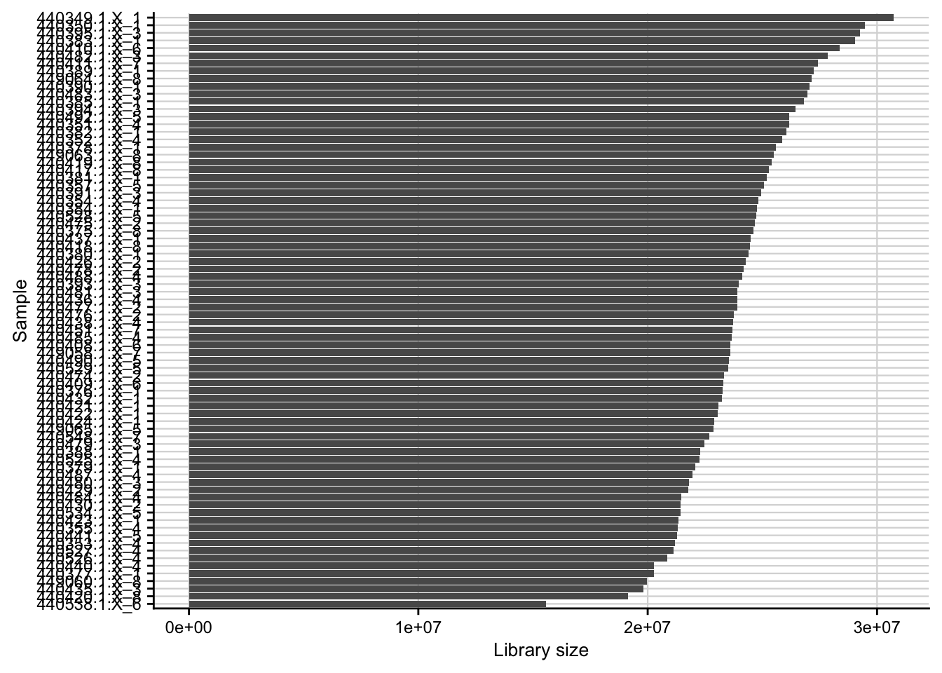
| Version | Author | Date |
|---|---|---|
| 6dbc304 | christianholland | 2020-12-20 |
Count distribution
Violin plots of the raw read counts for each of the samples.
count_matrix <- readRDS(here(data_path, "count_matrix.rds"))
meta <- readRDS(here(data_path, "meta_data.rds"))

count_matrix %>%
  tdy("gene", "sample", "count", meta) %>%
  arrange(nafld) %>%
  ggplot(aes(
    x = fct_reorder(sample, as.numeric(nafld)), y = log10(count + 1),
    group = sample, fill = nafld
  )) +
  geom_violin() +
  theme(
    axis.text.x = element_text(angle = 90, vjust = 0.5, hjust = 1),
    legend.position = "top"
  ) +
  labs(x = NULL) +
  my_theme(grid = "no", fsize = fz)
#> gather: reorganized (440349.1.X_1, 440350.1.X_1, 440351.1.X_4, 440352.1.X_4, 440353.1.X_4, …) into (sample, count) [was 17140x79, now 1336920x3]
#> left_join: added 7 columns (fibrosis, lobular_inflammation, nafld, gender, steatosis, …)
#>            > rows only in x           0
#>            > rows only in y  (        0)
#>            > matched rows     1,336,920
#>            >                 ===========
#>            > rows total       1,336,920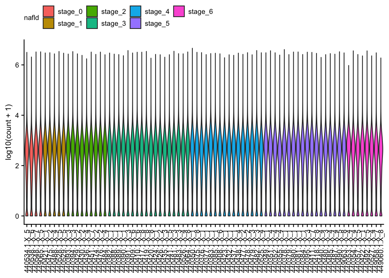
| Version | Author | Date |
|---|---|---|
| 6dbc304 | christianholland | 2020-12-20 |
PCA of raw data
PCA plot of raw read counts contextualized based on NAFLD stage. Before gene with a constant expression across all samples are removed and count values are transformed to log2 scale. Only the top 1000 most variable genes are used as features.
count_matrix <- readRDS(here(data_path, "count_matrix.rds"))
meta <- readRDS(here(data_path, "meta_data.rds"))

stopifnot(colnames(count_matrix) == meta$sample)

# remove constant expressed genes and transform to log2 scale
preprocessed_count_matrix <- preprocess_count_matrix(count_matrix)
#> Discarding 239 genes
#> Keeping 16901 genes


pca_result <- do_pca(preprocessed_count_matrix, meta, top_n_var_genes = 1000)
#> left_join: added 7 columns (fibrosis, lobular_inflammation, nafld, gender, steatosis, …)
#>            > rows only in x    0
#>            > rows only in y  ( 0)
#>            > matched rows     78
#>            >                 ====
#>            > rows total       78

plot_pca(pca_result, feature = "nafld") +
  my_theme(fsize = fz)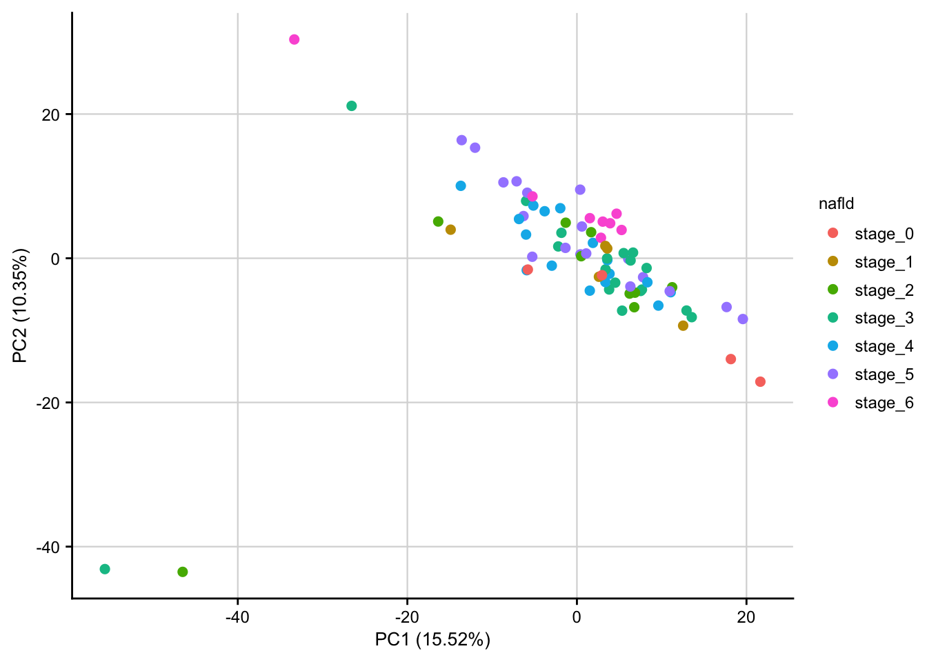
| Version | Author | Date |
|---|---|---|
| 6dbc304 | christianholland | 2020-12-20 |
Data processing
Normalization
Raw read counts are normalized by first filtering out lowly expressed genes, TMM normalization and finally logCPM transformation.
count_matrix <- readRDS(here(data_path, "count_matrix.rds"))
meta <- readRDS(here(data_path, "meta_data.rds"))

stopifnot(meta$sample == colnames(count_matrix))

dge_obj <- DGEList(count_matrix, group = meta$nafld)

# filter low read counts, TMM normalization and logCPM transformation
norm <- voom_normalization(dge_obj)
#> Discarding 1947 genes
#> Keeping 15193 genes

saveRDS(norm, here(output_path, "normalized_expression.rds"))
PCA of normalized data
PCA plot of normalized expression data contextualized based on the NAFLD stage. Only the top 1000 most variable genes are used as features.
expr <- readRDS(here(output_path, "normalized_expression.rds"))
meta <- readRDS(here(data_path, "meta_data.rds"))

pca_result <- do_pca(expr, meta, top_n_var_genes = 1000)
#> left_join: added 7 columns (fibrosis, lobular_inflammation, nafld, gender, steatosis, …)
#>            > rows only in x    0
#>            > rows only in y  ( 0)
#>            > matched rows     78
#>            >                 ====
#>            > rows total       78

saveRDS(pca_result, here(output_path, "pca_result.rds"))

plot_pca(pca_result, feature = "nafld") +
  my_theme(fsize = fz)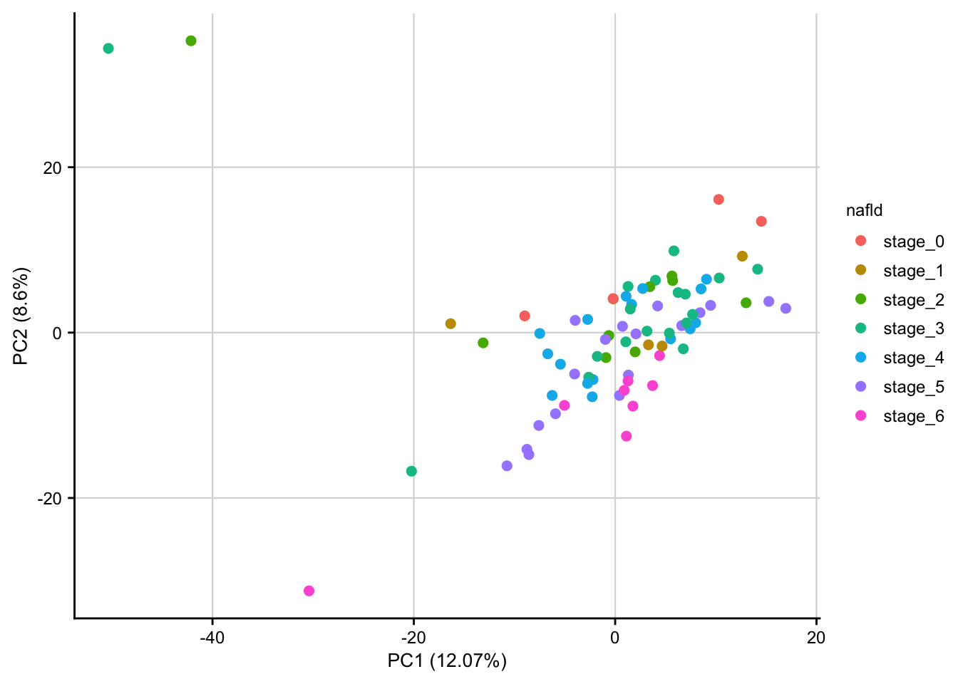
| Version | Author | Date |
|---|---|---|
| 6dbc304 | christianholland | 2020-12-20 |
Differential gene expression analysis
Running limma
Differential gene expression analysis via limma with the aim to identify the transcriptomic signatures of different NAFLD stages.
# load expression and meta data
expr <- readRDS(here(output_path, "normalized_expression.rds"))
meta <- readRDS(here(data_path, "meta_data.rds"))

stopifnot(colnames(expr) == meta$sample)

# build design matrix
design <- model.matrix(~ 0 + nafld, data = meta)
rownames(design) <- meta$sample
colnames(design) <- levels(meta$nafld)


# define contrasts
contrasts <- makeContrasts(
  stage_1_vs_0 = stage_1 - stage_0,
  stage_2_vs_0 = stage_2 - stage_0,
  stage_3_vs_0 = stage_3 - stage_0,
  stage_4_vs_0 = stage_4 - stage_0,
  stage_5_vs_0 = stage_5 - stage_0,
  stage_6_vs_0 = stage_6 - stage_0,
  levels = design
)

limma_result <- run_limma(expr, design, contrasts) %>%
  assign_deg()
#> Warning: `tbl_df()` is deprecated as of dplyr 1.0.0.
#> Please use `tibble::as_tibble()` instead.
#> This warning is displayed once every 8 hours.
#> Call `lifecycle::last_warnings()` to see where this warning was generated.
#> select: renamed 3 variables (contrast, logFC, pval) and dropped one variable
#> group_by: one grouping variable (contrast)
#> mutate (grouped): new variable 'fdr' (double) with 38,517 unique values and 0% NA
#> ungroup: no grouping variables
#> mutate: new variable 'regulation' (character) with 3 unique values and 0% NA
#> mutate: converted 'regulation' from character to factor (0 new NA)

deg_df <- limma_result %>%
  mutate(contrast_reference = "stage_0")
#> mutate: new variable 'contrast_reference' (character) with one unique value and 0% NA

saveRDS(deg_df, here(output_path, "limma_result.rds"))
Volcano plots
Volcano plots visualizing the transcriptomic signatures of different NAFLD stages.
df <- readRDS(here(output_path, "limma_result.rds"))

df %>%
  filter(contrast_reference == "stage_0") %>%
  plot_volcano() +
  my_theme(grid = "y", fsize = fz)
#> filter: no rows removed
#> rename: renamed one variable (p)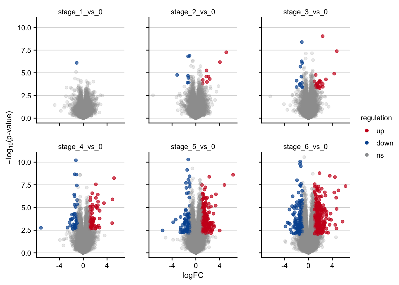
| Version | Author | Date |
|---|---|---|
| 6dbc304 | christianholland | 2020-12-20 |
Time spend to execute this analysis: 00:22 minutes.
sessionInfo()
#> R version 4.0.2 (2020-06-22)
#> Platform: x86_64-apple-darwin17.0 (64-bit)
#> Running under: macOS Mojave 10.14.5
#>
#> Matrix products: default
#> BLAS:   /Library/Frameworks/R.framework/Versions/4.0/Resources/lib/libRblas.dylib
#> LAPACK: /Library/Frameworks/R.framework/Versions/4.0/Resources/lib/libRlapack.dylib
#>
#> locale:
#> [1] en_US.UTF-8/en_US.UTF-8/en_US.UTF-8/C/en_US.UTF-8/en_US.UTF-8
#>
#> attached base packages:
#> [1] stats     graphics  grDevices datasets  utils     methods   base
#>
#> other attached packages:
#>  [1] lemon_0.4.5              cowplot_1.1.0            AachenColorPalette_1.1.2
#>  [4] biobroom_1.20.0          broom_0.7.3              edgeR_3.30.3
#>  [7] limma_3.44.3             here_1.0.1               tidylog_1.0.2
#> [10] forcats_0.5.0            stringr_1.4.0            dplyr_1.0.2
#> [13] purrr_0.3.4              readr_1.4.0              tidyr_1.1.2
#> [16] tibble_3.0.4             ggplot2_3.3.2            tidyverse_1.3.0
#> [19] workflowr_1.6.2
#>
#> loaded via a namespace (and not attached):
#>  [1] Biobase_2.48.0      httr_1.4.2          jsonlite_1.7.2
#>  [4] modelr_0.1.8        assertthat_0.2.1    renv_0.12.3
#>  [7] cellranger_1.1.0    yaml_2.2.1          pillar_1.4.7
#> [10] backports_1.2.1     lattice_0.20-41     glue_1.4.2
#> [13] digest_0.6.27       promises_1.1.1      rvest_0.3.6
#> [16] colorspace_2.0-0    htmltools_0.5.0     httpuv_1.5.4
#> [19] plyr_1.8.6          clisymbols_1.2.0    pkgconfig_2.0.3
#> [22] haven_2.3.1         scales_1.1.1        whisker_0.4
#> [25] later_1.1.0.1       git2r_0.27.1        farver_2.0.3
#> [28] generics_0.1.0      ellipsis_0.3.1      withr_2.3.0
#> [31] BiocGenerics_0.34.0 cli_2.2.0           magrittr_2.0.1
#> [34] crayon_1.3.4        readxl_1.3.1        evaluate_0.14
#> [37] fs_1.5.0            fansi_0.4.1         xml2_1.3.2
#> [40] tools_4.0.2         hms_0.5.3           lifecycle_0.2.0
#> [43] munsell_0.5.0       reprex_0.3.0        locfit_1.5-9.4
#> [46] compiler_4.0.2      rlang_0.4.9         grid_4.0.2
#> [49] rstudioapi_0.13     labeling_0.4.2      rmarkdown_2.6
#> [52] codetools_0.2-16    gtable_0.3.0        DBI_1.1.0
#> [55] R6_2.5.0            gridExtra_2.3       lubridate_1.7.9.2
#> [58] knitr_1.30          rprojroot_2.0.2     stringi_1.5.3
#> [61] parallel_4.0.2      Rcpp_1.0.5          vctrs_0.3.6
#> [64] dbplyr_2.0.0        tidyselect_1.1.0    xfun_0.19