Main types of joins
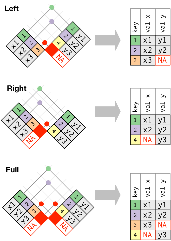
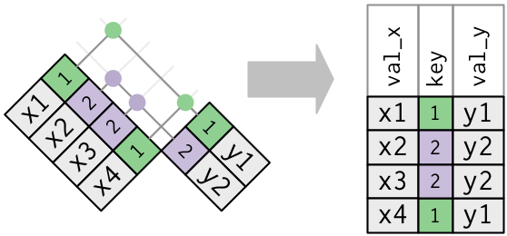
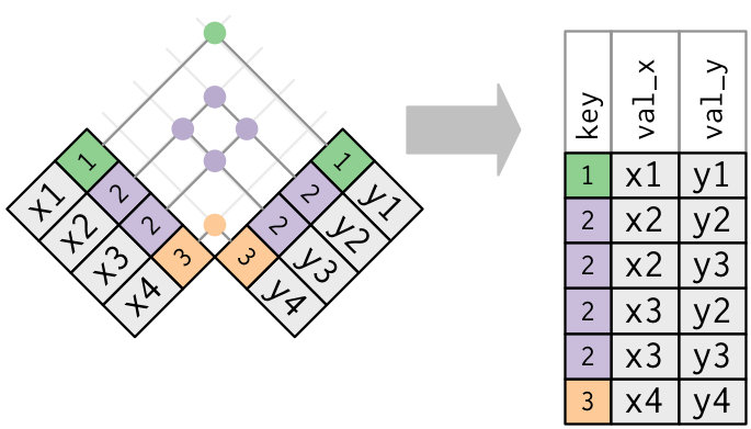
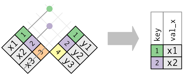
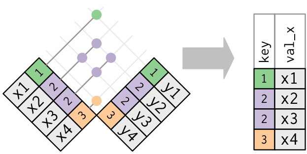
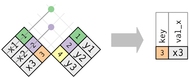
Mutating joins, which add new variables to one data frame from matching observations in another.
Filtering joins, which filter observations from one data frame based on whether or not they match an observation in the other table.
Set operations, which treat observations as if they were set elements.
Dataset
These are the datasets we will be using to learn about joins which come from the nycflights13 package.
airlineslets you look up the full carrier name from its abbreviated code:airlines #> # A tibble: 16 x 2 #> carrier name #> <chr> <chr> #> 1 9E Endeavor Air Inc. #> 2 AA American Airlines Inc. #> 3 AS Alaska Airlines Inc. #> 4 B6 JetBlue Airways #> 5 DL Delta Air Lines Inc. #> 6 EV ExpressJet Airlines Inc. #> 7 F9 Frontier Airlines Inc. #> 8 FL AirTran Airways Corporation #> 9 HA Hawaiian Airlines Inc. #> 10 MQ Envoy Air #> 11 OO SkyWest Airlines Inc. #> 12 UA United Air Lines Inc. #> 13 US US Airways Inc. #> 14 VX Virgin America #> 15 WN Southwest Airlines Co. #> 16 YV Mesa Airlines Inc.airportsgives information about each airport, identified by thefaaairport code:airports #> # A tibble: 1,458 x 8 #> faa name lat lon alt tz dst tzone #> <chr> <chr> <dbl> <dbl> <dbl> <dbl> <chr> <chr> #> 1 04G Lansdowne Airport 41.1 -80.6 1044 -5 A America/New_Yo~ #> 2 06A Moton Field Municipal A~ 32.5 -85.7 264 -6 A America/Chicago #> 3 06C Schaumburg Regional 42.0 -88.1 801 -6 A America/Chicago #> 4 06N Randall Airport 41.4 -74.4 523 -5 A America/New_Yo~ #> 5 09J Jekyll Island Airport 31.1 -81.4 11 -5 A America/New_Yo~ #> 6 0A9 Elizabethton Municipal ~ 36.4 -82.2 1593 -5 A America/New_Yo~ #> 7 0G6 Williams County Airport 41.5 -84.5 730 -5 A America/New_Yo~ #> 8 0G7 Finger Lakes Regional A~ 42.9 -76.8 492 -5 A America/New_Yo~ #> 9 0P2 Shoestring Aviation Air~ 39.8 -76.6 1000 -5 U America/New_Yo~ #> 10 0S9 Jefferson County Intl 48.1 -123. 108 -8 A America/Los_An~ #> # ... with 1,448 more rowsplanesgives information about each plane, identified by itstailnum:planes #> # A tibble: 3,322 x 9 #> tailnum year type manufacturer model engines seats speed engine #> <chr> <int> <chr> <chr> <chr> <int> <int> <int> <chr> #> 1 N10156 2004 Fixed wing m~ EMBRAER EMB-1~ 2 55 NA Turbo-~ #> 2 N102UW 1998 Fixed wing m~ AIRBUS INDUST~ A320-~ 2 182 NA Turbo-~ #> 3 N103US 1999 Fixed wing m~ AIRBUS INDUST~ A320-~ 2 182 NA Turbo-~ #> 4 N104UW 1999 Fixed wing m~ AIRBUS INDUST~ A320-~ 2 182 NA Turbo-~ #> 5 N10575 2002 Fixed wing m~ EMBRAER EMB-1~ 2 55 NA Turbo-~ #> 6 N105UW 1999 Fixed wing m~ AIRBUS INDUST~ A320-~ 2 182 NA Turbo-~ #> 7 N107US 1999 Fixed wing m~ AIRBUS INDUST~ A320-~ 2 182 NA Turbo-~ #> 8 N108UW 1999 Fixed wing m~ AIRBUS INDUST~ A320-~ 2 182 NA Turbo-~ #> 9 N109UW 1999 Fixed wing m~ AIRBUS INDUST~ A320-~ 2 182 NA Turbo-~ #> 10 N110UW 1999 Fixed wing m~ AIRBUS INDUST~ A320-~ 2 182 NA Turbo-~ #> # ... with 3,312 more rowsweathergives the weather at each NYC airport for each hour:weather #> # A tibble: 26,115 x 15 #> origin year month day hour temp dewp humid wind_dir wind_speed #> <chr> <int> <int> <int> <int> <dbl> <dbl> <dbl> <dbl> <dbl> #> 1 EWR 2013 1 1 1 39.0 26.1 59.4 270 10.4 #> 2 EWR 2013 1 1 2 39.0 27.0 61.6 250 8.06 #> 3 EWR 2013 1 1 3 39.0 28.0 64.4 240 11.5 #> 4 EWR 2013 1 1 4 39.9 28.0 62.2 250 12.7 #> 5 EWR 2013 1 1 5 39.0 28.0 64.4 260 12.7 #> 6 EWR 2013 1 1 6 37.9 28.0 67.2 240 11.5 #> 7 EWR 2013 1 1 7 39.0 28.0 64.4 240 15.0 #> 8 EWR 2013 1 1 8 39.9 28.0 62.2 250 10.4 #> 9 EWR 2013 1 1 9 39.9 28.0 62.2 260 15.0 #> 10 EWR 2013 1 1 10 41 28.0 59.6 260 13.8 #> # ... with 26,105 more rows, and 5 more variables: wind_gust <dbl>, #> # precip <dbl>, pressure <dbl>, visib <dbl>, time_hour <dttm>flightsgives the flights departing a NYC airport:flights #> # A tibble: 336,776 x 19 #> year month day dep_time sched_dep_time dep_delay arr_time sched_arr_time #> <int> <int> <int> <int> <int> <dbl> <int> <int> #> 1 2013 1 1 517 515 2 830 819 #> 2 2013 1 1 533 529 4 850 830 #> 3 2013 1 1 542 540 2 923 850 #> 4 2013 1 1 544 545 -1 1004 1022 #> 5 2013 1 1 554 600 -6 812 837 #> 6 2013 1 1 554 558 -4 740 728 #> 7 2013 1 1 555 600 -5 913 854 #> 8 2013 1 1 557 600 -3 709 723 #> 9 2013 1 1 557 600 -3 838 846 #> 10 2013 1 1 558 600 -2 753 745 #> # ... with 336,766 more rows, and 11 more variables: arr_delay <dbl>, #> # carrier <chr>, flight <int>, tailnum <chr>, origin <chr>, dest <chr>, #> # air_time <dbl>, distance <dbl>, hour <dbl>, minute <dbl>, time_hour <dttm>
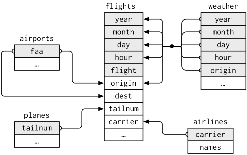
For nycflights13:
flightsconnects toplanesvia a single variable,tailnum.flightsconnects toairlinesthrough thecarriervariable.flightsconnects toairportsin two ways: via theoriginanddestvariables.flightsconnects toweatherviaorigin(the location), andyear,month,dayandhour(the time).
Exercises
Imagine you wanted to draw (approximately) the route each plane flies from its origin to its destination. What variables would you need? What tables would you need to combine?
We would need the origin and dest from
flightsand the lat and lon for each origin / dest fromairports.I forgot to draw the relationship between
weatherandairports. What is the relationship and how should it appear in the diagram?weatherhas origin, andairportshas faa. These could be joined to get all weather conditions for each day and each hour in the dataset.weatheronly contains information for the origin (NYC) airports. If it contained weather records for all airports in the USA, what additional relation would it define withflights?There would be a relation with dest.
We know that some days of the year are “special”, and fewer people than usual fly on them. How might you represent that data as a data frame? What would be the primary keys of that table? How would it connect to the existing tables?
I would have a table called
holidaysand it would have a year, month and day variable that can be used to connect to flights, and weather.