Chapter 3 - Data Transformation with dplyr
Vebash Naidoo
17/09/2020
Last updated: 2020-11-07
Checks: 7 0
Knit directory: r4ds_book/
This reproducible R Markdown analysis was created with workflowr (version 1.6.2). The Checks tab describes the reproducibility checks that were applied when the results were created. The Past versions tab lists the development history.
Great! Since the R Markdown file has been committed to the Git repository, you know the exact version of the code that produced these results.
Great job! The global environment was empty. Objects defined in the global environment can affect the analysis in your R Markdown file in unknown ways. For reproduciblity it’s best to always run the code in an empty environment.
The command set.seed(20200814) was run prior to running the code in the R Markdown file. Setting a seed ensures that any results that rely on randomness, e.g. subsampling or permutations, are reproducible.
Great job! Recording the operating system, R version, and package versions is critical for reproducibility.
Nice! There were no cached chunks for this analysis, so you can be confident that you successfully produced the results during this run.
Great job! Using relative paths to the files within your workflowr project makes it easier to run your code on other machines.
Great! You are using Git for version control. Tracking code development and connecting the code version to the results is critical for reproducibility.
The results in this page were generated with repository version 9440e66. See the Past versions tab to see a history of the changes made to the R Markdown and HTML files.
Note that you need to be careful to ensure that all relevant files for the analysis have been committed to Git prior to generating the results (you can use wflow_publish or wflow_git_commit). workflowr only checks the R Markdown file, but you know if there are other scripts or data files that it depends on. Below is the status of the Git repository when the results were generated:
Ignored files:
    Ignored:    .Rproj.user/

Untracked files:
    Untracked:  analysis/images/
    Untracked:  code_snipp.txt
Note that any generated files, e.g. HTML, png, CSS, etc., are not included in this status report because it is ok for generated content to have uncommitted changes.
These are the previous versions of the repository in which changes were made to the R Markdown (analysis/ch3_dplyr.Rmd) and HTML (docs/ch3_dplyr.html) files. If you’ve configured a remote Git repository (see ?wflow_git_remote), click on the hyperlinks in the table below to view the files as they were in that past version.
| File | Version | Author | Date | Message |
|---|---|---|---|---|
| html | 274005c | sciencificity | 2020-11-06 | Build site. |
| html | 60e7ce2 | sciencificity | 2020-11-02 | Build site. |
| html | db5a796 | sciencificity | 2020-11-01 | Build site. |
| html | d8813e9 | sciencificity | 2020-11-01 | Build site. |
| html | bf15f3b | sciencificity | 2020-11-01 | Build site. |
| html | 0aef1b0 | sciencificity | 2020-10-31 | Build site. |
| html | bdc0881 | sciencificity | 2020-10-26 | Build site. |
| html | 8224544 | sciencificity | 2020-10-26 | Build site. |
| html | 2f8dcc0 | sciencificity | 2020-10-25 | Build site. |
| html | 61e2324 | sciencificity | 2020-10-25 | Build site. |
| html | 570c0bb | sciencificity | 2020-10-22 | Build site. |
| html | cfbefe6 | sciencificity | 2020-10-21 | Build site. |
| html | 4497db4 | sciencificity | 2020-10-18 | Build site. |
| html | 1a3bebe | sciencificity | 2020-10-18 | Build site. |
| html | ce8c214 | sciencificity | 2020-10-16 | Build site. |
| html | 1fa6c06 | sciencificity | 2020-10-16 | Build site. |
| Rmd | 3b67e92 | sciencificity | 2020-10-16 | completed ch 3 |
| html | 9ae5861 | sciencificity | 2020-10-13 | Build site. |
| Rmd | d9de836 | sciencificity | 2020-10-13 | added more content Ch 3 |
| html | 76c2bc4 | sciencificity | 2020-10-10 | Build site. |
| Rmd | bbb6cd2 | sciencificity | 2020-10-10 | added Ch 4 section |
| html | 226cd16 | sciencificity | 2020-10-10 | Build site. |
| Rmd | ae71e8e | sciencificity | 2020-10-10 | added Ch 4 section |
library(tidyverse)
library(flair)
library(nycflights13)
library(palmerpenguins)
library(gt)
library(skimr)
library(emo)
library(tidyquant)
library(lubridate)
library(magrittr)
theme_set(theme_tq())
Filter rows
filter() is the verb used to subset rows in a dataframe based on their values - i.e. we take a dataset and we say hey, give me back data that looks like it fulfils this condition(s).
The nycflights13 package has flights for the year 2013 where the departure was from an airport in New York City. You will notice the %>% which we used in the ggplot chapter too. If you can’t recall what it does for now ignore it and just have a look at the data contained in the dataset.
Aside: the pipe into gt() is to print out a neat table 😄.
flights %>%
  head(4) %>%
  gt()
| year | month | day | dep_time | sched_dep_time | dep_delay | arr_time | sched_arr_time | arr_delay | carrier | flight | tailnum | origin | dest | air_time | distance | hour | minute | time_hour |
|---|---|---|---|---|---|---|---|---|---|---|---|---|---|---|---|---|---|---|
| 2013 | 1 | 1 | 517 | 515 | 2 | 830 | 819 | 11 | UA | 1545 | N14228 | EWR | IAH | 227 | 1400 | 5 | 15 | 2013-01-01 05:00:00 |
| 2013 | 1 | 1 | 533 | 529 | 4 | 850 | 830 | 20 | UA | 1714 | N24211 | LGA | IAH | 227 | 1416 | 5 | 29 | 2013-01-01 05:00:00 |
| 2013 | 1 | 1 | 542 | 540 | 2 | 923 | 850 | 33 | AA | 1141 | N619AA | JFK | MIA | 160 | 1089 | 5 | 40 | 2013-01-01 05:00:00 |
| 2013 | 1 | 1 | 544 | 545 | -1 | 1004 | 1022 | -18 | B6 | 725 | N804JB | JFK | BQN | 183 | 1576 | 5 | 45 | 2013-01-01 05:00:00 |
flights %>%
  count(origin, sort=TRUE) %>%
gt()| origin | n |
|---|---|
| EWR | 120835 |
| JFK | 111279 |
| LGA | 104662 |
Let’s filter all flights that occurred on Jan 1. The syntax for filter is filter(df, some_condition_s)
filter(flights, month == 1, day == 1)
# A tibble: 842 x 19
    year month   day dep_time sched_dep_time dep_delay arr_time sched_arr_time
   <int> <int> <int>    <int>          <int>     <dbl>    <int>          <int>
 1  2013     1     1      517            515         2      830            819
 2  2013     1     1      533            529         4      850            830
 3  2013     1     1      542            540         2      923            850
 4  2013     1     1      544            545        -1     1004           1022
 5  2013     1     1      554            600        -6      812            837
 6  2013     1     1      554            558        -4      740            728
 7  2013     1     1      555            600        -5      913            854
 8  2013     1     1      557            600        -3      709            723
 9  2013     1     1      557            600        -3      838            846
10  2013     1     1      558            600        -2      753            745
# ... with 832 more rows, and 11 more variables: arr_delay <dbl>,
#   carrier <chr>, flight <int>, tailnum <chr>, origin <chr>, dest <chr>,
#   air_time <dbl>, distance <dbl>, hour <dbl>, minute <dbl>, time_hour <dttm>
Notice the == for comparison
| sign | meaning |
|---|---|
| > | greater than |
| >= | greater than or equal to |
| < | less than |
| <= | less than or equal to |
| == | equal to |
| != | not equal to |
Okay, truly the {palmerpenguins} data is going to become the new iris! But come on’ who doesn’t love penguins! Just try and keep me away from Boulders Beach in Cape Town when I’m there visiting …
penguins %>%
  head(10) %>%
gt()| species | island | bill_length_mm | bill_depth_mm | flipper_length_mm | body_mass_g | sex | year |
|---|---|---|---|---|---|---|---|
| Adelie | Torgersen | 39.1 | 18.7 | 181 | 3750 | male | 2007 |
| Adelie | Torgersen | 39.5 | 17.4 | 186 | 3800 | female | 2007 |
| Adelie | Torgersen | 40.3 | 18.0 | 195 | 3250 | female | 2007 |
| Adelie | Torgersen | NA | NA | NA | NA | NA | 2007 |
| Adelie | Torgersen | 36.7 | 19.3 | 193 | 3450 | female | 2007 |
| Adelie | Torgersen | 39.3 | 20.6 | 190 | 3650 | male | 2007 |
| Adelie | Torgersen | 38.9 | 17.8 | 181 | 3625 | female | 2007 |
| Adelie | Torgersen | 39.2 | 19.6 | 195 | 4675 | male | 2007 |
| Adelie | Torgersen | 34.1 | 18.1 | 193 | 3475 | NA | 2007 |
| Adelie | Torgersen | 42.0 | 20.2 | 190 | 4250 | NA | 2007 |
Ok, what types of penguins are there?
penguins %>%
  count(species, sort=TRUE)
# A tibble: 3 x 2
species n
<fct> <int>
1 Adelie 152
2 Gentoo 124
3 Chinstrap 68Let’s filter out Gentoo with bill_depth_mm bigger than 17mm, using some of the operations we learnt.
# lets us save the filter result and
# prints it out ... the extra brackets on the
# outside of the entire code block does that
(gentoo <- filter(penguins, species == 'Gentoo',
       bill_depth_mm > 17))
# A tibble: 3 x 8
  species island bill_length_mm bill_depth_mm flipper_length_~ body_mass_g sex
  <fct>   <fct>           <dbl>         <dbl>            <int>       <int> <fct>
1 Gentoo  Biscoe           44.4          17.3              219        5250 male
2 Gentoo  Biscoe           50.8          17.3              228        5600 male
3 Gentoo  Biscoe           52.2          17.1              228        5400 male
# ... with 1 more variable: year <int>
Surprising results
Floats are saved a bit differently and hence can cause some unexpected behaviour.
sqrt(2) ^ 2 == 2[1] FALSE1 / 49 * 49 == 1[1] FALSEUse near() to give you if these are indeed nearly same.
near(sqrt(2) ^ 2, 2)
[1] TRUE
near(1 / 49 * 49, 1)
[1] TRUE
Logic
When we explore data we often want to filter data where one condition is true and another is also true. E.g. Which days experienced a thunder storm where a thunder storm was predicted by the Meteorologists.
In R we use logic operators to combine comparisons and get us the data we’re looking for.
| sign | meaning |
|---|---|
| | | Or |
| & | And |
| ! | Not |
Let’s say we want only flights that occurred in Nov and Dec of 2013:
filter(flights, month == 11 | month == 12)
# A tibble: 55,403 x 19
    year month   day dep_time sched_dep_time dep_delay arr_time sched_arr_time
   <int> <int> <int>    <int>          <int>     <dbl>    <int>          <int>
 1  2013    11     1        5           2359         6      352            345
 2  2013    11     1       35           2250       105      123           2356
 3  2013    11     1      455            500        -5      641            651
 4  2013    11     1      539            545        -6      856            827
 5  2013    11     1      542            545        -3      831            855
 6  2013    11     1      549            600       -11      912            923
 7  2013    11     1      550            600       -10      705            659
 8  2013    11     1      554            600        -6      659            701
 9  2013    11     1      554            600        -6      826            827
10  2013    11     1      554            600        -6      749            751
# ... with 55,393 more rows, and 11 more variables: arr_delay <dbl>,
#   carrier <chr>, flight <int>, tailnum <chr>, origin <chr>, dest <chr>,
#   air_time <dbl>, distance <dbl>, hour <dbl>, minute <dbl>, time_hour <dttm>
We have to repeat the month == part for each comparison.
You may think that you can just say month == (11 | 12) but unfortunately that does not work.
(filtered_fl <- filter(flights, month == (11 | 12)))
# A tibble: 27,004 x 19
    year month   day dep_time sched_dep_time dep_delay arr_time sched_arr_time
   <int> <int> <int>    <int>          <int>     <dbl>    <int>          <int>
 1  2013     1     1      517            515         2      830            819
 2  2013     1     1      533            529         4      850            830
 3  2013     1     1      542            540         2      923            850
 4  2013     1     1      544            545        -1     1004           1022
 5  2013     1     1      554            600        -6      812            837
 6  2013     1     1      554            558        -4      740            728
 7  2013     1     1      555            600        -5      913            854
 8  2013     1     1      557            600        -3      709            723
 9  2013     1     1      557            600        -3      838            846
10  2013     1     1      558            600        -2      753            745
# ... with 26,994 more rows, and 11 more variables: arr_delay <dbl>,
#   carrier <chr>, flight <int>, tailnum <chr>, origin <chr>, dest <chr>,
#   air_time <dbl>, distance <dbl>, hour <dbl>, minute <dbl>, time_hour <dttm>
Note that the result is unexpected - the tibble returned contains the month == 1 which is January, and should not be in our returned dataset! The (11 | 12) evaluates to TRUE which internally is represented as 1 hence we then look at month == 1. To see this lets load the flights dataframe and filter Jan again. Notice that the number of rows is identical to the number of rows in the filtered filtered_fl which is 27004.
flights %>%
  filter(month == 1)
# A tibble: 27,004 x 19
year month day dep_time sched_dep_time dep_delay arr_time sched_arr_time
<int> <int> <int> <int> <int> <dbl> <int> <int>
1 2013 1 1 517 515 2 830 819
2 2013 1 1 533 529 4 850 830
3 2013 1 1 542 540 2 923 850
4 2013 1 1 544 545 -1 1004 1022
5 2013 1 1 554 600 -6 812 837
6 2013 1 1 554 558 -4 740 728
7 2013 1 1 555 600 -5 913 854
8 2013 1 1 557 600 -3 709 723
9 2013 1 1 557 600 -3 838 846
10 2013 1 1 558 600 -2 753 745
# ... with 26,994 more rows, and 11 more variables: arr_delay <dbl>,
# carrier <chr>, flight <int>, tailnum <chr>, origin <chr>, dest <chr>,
# air_time <dbl>, distance <dbl>, hour <dbl>, minute <dbl>, time_hour <dttm>We can also use the %in% operator instead of repeating the month ==.
filter(flights, month %in% c(11, 12))# A tibble: 55,403 x 19
year month day dep_time sched_dep_time dep_delay arr_time sched_arr_time
<int> <int> <int> <int> <int> <dbl> <int> <int>
1 2013 11 1 5 2359 6 352 345
2 2013 11 1 35 2250 105 123 2356
3 2013 11 1 455 500 -5 641 651
4 2013 11 1 539 545 -6 856 827
5 2013 11 1 542 545 -3 831 855
6 2013 11 1 549 600 -11 912 923
7 2013 11 1 550 600 -10 705 659
8 2013 11 1 554 600 -6 659 701
9 2013 11 1 554 600 -6 826 827
10 2013 11 1 554 600 -6 749 751
# ... with 55,393 more rows, and 11 more variables: arr_delay <dbl>,
# carrier <chr>, flight <int>, tailnum <chr>, origin <chr>, dest <chr>,
# air_time <dbl>, distance <dbl>, hour <dbl>, minute <dbl>, time_hour <dttm>If you need the opposite of this i.e. the not in operator it’s a bit more tricky.
You can make your own function for this.
'%!in%' <- function(x,y)!('%in%'(x,y)) # method 1
'%ni%' <- Negate('%in%') # method 2
filter(flights, month %ni% c(11, 12))
# A tibble: 281,373 x 19
year month day dep_time sched_dep_time dep_delay arr_time sched_arr_time
<int> <int> <int> <int> <int> <dbl> <int> <int>
1 2013 1 1 517 515 2 830 819
2 2013 1 1 533 529 4 850 830
3 2013 1 1 542 540 2 923 850
4 2013 1 1 544 545 -1 1004 1022
5 2013 1 1 554 600 -6 812 837
6 2013 1 1 554 558 -4 740 728
7 2013 1 1 555 600 -5 913 854
8 2013 1 1 557 600 -3 709 723
9 2013 1 1 557 600 -3 838 846
10 2013 1 1 558 600 -2 753 745
# ... with 281,363 more rows, and 11 more variables: arr_delay <dbl>,
# carrier <chr>, flight <int>, tailnum <chr>, origin <chr>, dest <chr>,
# air_time <dbl>, distance <dbl>, hour <dbl>, minute <dbl>, time_hour <dttm>Aside: Some penguin fun …
Let’s see if we can explore our data through filtering.
# Get all penguins where the species is anything
# other than Adelie
filter(penguins, species %ni% ('Adelie'))
# A tibble: 192 x 8
species island bill_length_mm bill_depth_mm flipper_length_~ body_mass_g
<fct> <fct> <dbl> <dbl> <int> <int>
1 Gentoo Biscoe 46.1 13.2 211 4500
2 Gentoo Biscoe 50 16.3 230 5700
3 Gentoo Biscoe 48.7 14.1 210 4450
4 Gentoo Biscoe 50 15.2 218 5700
5 Gentoo Biscoe 47.6 14.5 215 5400
6 Gentoo Biscoe 46.5 13.5 210 4550
7 Gentoo Biscoe 45.4 14.6 211 4800
8 Gentoo Biscoe 46.7 15.3 219 5200
9 Gentoo Biscoe 43.3 13.4 209 4400
10 Gentoo Biscoe 46.8 15.4 215 5150
# ... with 182 more rows, and 2 more variables: sex <fct>, year <int>The skim function also works great in conjunction with filter. I am going to use the pipe again which we tackle later in R4DS. For now when you see %>% read it as and then e.g. Take this df and then filter out data that meets the condition and then show me a summary.
    df %>%
      filter(some_col meets some condition) %>%
      summary(avg_col = mean(some_col))
penguins %>%
  filter(species == "Chinstrap") %>%
skim()| Name | Piped data |
| Number of rows | 68 |
| Number of columns | 8 |
| _______________________ | |
| Column type frequency: | |
| factor | 3 |
| numeric | 5 |
| ________________________ | |
| Group variables | None |
Variable type: factor
| skim_variable | n_missing | complete_rate | ordered | n_unique | top_counts |
|---|---|---|---|---|---|
| species | 0 | 1 | FALSE | 1 | Chi: 68, Ade: 0, Gen: 0 |
| island | 0 | 1 | FALSE | 1 | Dre: 68, Bis: 0, Tor: 0 |
| sex | 0 | 1 | FALSE | 2 | fem: 34, mal: 34 |
Variable type: numeric
| skim_variable | n_missing | complete_rate | mean | sd | p0 | p25 | p50 | p75 | p100 | hist |
|---|---|---|---|---|---|---|---|---|---|---|
| bill_length_mm | 0 | 1 | 48.83 | 3.34 | 40.9 | 46.35 | 49.55 | 51.08 | 58.0 | ▂▇▇▅▁ |
| bill_depth_mm | 0 | 1 | 18.42 | 1.14 | 16.4 | 17.50 | 18.45 | 19.40 | 20.8 | ▅▇▇▆▂ |
| flipper_length_mm | 0 | 1 | 195.82 | 7.13 | 178.0 | 191.00 | 196.00 | 201.00 | 212.0 | ▁▅▇▅▂ |
| body_mass_g | 0 | 1 | 3733.09 | 384.34 | 2700.0 | 3487.50 | 3700.00 | 3950.00 | 4800.0 | ▁▅▇▃▁ |
| year | 0 | 1 | 2007.97 | 0.86 | 2007.0 | 2007.00 | 2008.00 | 2009.00 | 2009.0 | ▇▁▆▁▇ |
Let’s see if the Chinstrap penguins with a body mass above the mean are more likely male / female / equally represented?
The pipe way:
penguins %>%
  filter(species == "Chinstrap") %>%
  filter(body_mass_g > mean(body_mass_g)) %>%
skim()| Name | Piped data |
| Number of rows | 31 |
| Number of columns | 8 |
| _______________________ | |
| Column type frequency: | |
| factor | 3 |
| numeric | 5 |
| ________________________ | |
| Group variables | None |
Variable type: factor
| skim_variable | n_missing | complete_rate | ordered | n_unique | top_counts |
|---|---|---|---|---|---|
| species | 0 | 1 | FALSE | 1 | Chi: 31, Ade: 0, Gen: 0 |
| island | 0 | 1 | FALSE | 1 | Dre: 31, Bis: 0, Tor: 0 |
| sex | 0 | 1 | FALSE | 2 | mal: 25, fem: 6 |
Variable type: numeric
| skim_variable | n_missing | complete_rate | mean | sd | p0 | p25 | p50 | p75 | p100 | hist |
|---|---|---|---|---|---|---|---|---|---|---|
| bill_length_mm | 0 | 1 | 50.38 | 2.30 | 45.2 | 49.25 | 50.6 | 51.80 | 55.8 | ▂▃▇▅▁ |
| bill_depth_mm | 0 | 1 | 19.07 | 0.90 | 16.8 | 18.40 | 19.0 | 19.65 | 20.8 | ▁▅▆▇▂ |
| flipper_length_mm | 0 | 1 | 200.77 | 5.47 | 193.0 | 196.50 | 201.0 | 204.00 | 212.0 | ▇▅▇▃▃ |
| body_mass_g | 0 | 1 | 4055.65 | 267.14 | 3750.0 | 3825.00 | 4000.0 | 4150.00 | 4800.0 | ▇▅▁▂▁ |
| year | 0 | 1 | 2008.00 | 0.86 | 2007.0 | 2007.00 | 2008.0 | 2009.00 | 2009.0 | ▇▁▆▁▇ |
We get the same using the non-piped way.
skim(filter(filter(penguins, species == "Chinstrap"),
body_mass_g > mean(body_mass_g))) | Name | filter(…) |
| Number of rows | 31 |
| Number of columns | 8 |
| _______________________ | |
| Column type frequency: | |
| factor | 3 |
| numeric | 5 |
| ________________________ | |
| Group variables | None |
Variable type: factor
| skim_variable | n_missing | complete_rate | ordered | n_unique | top_counts |
|---|---|---|---|---|---|
| species | 0 | 1 | FALSE | 1 | Chi: 31, Ade: 0, Gen: 0 |
| island | 0 | 1 | FALSE | 1 | Dre: 31, Bis: 0, Tor: 0 |
| sex | 0 | 1 | FALSE | 2 | mal: 25, fem: 6 |
Variable type: numeric
| skim_variable | n_missing | complete_rate | mean | sd | p0 | p25 | p50 | p75 | p100 | hist |
|---|---|---|---|---|---|---|---|---|---|---|
| bill_length_mm | 0 | 1 | 50.38 | 2.30 | 45.2 | 49.25 | 50.6 | 51.80 | 55.8 | ▂▃▇▅▁ |
| bill_depth_mm | 0 | 1 | 19.07 | 0.90 | 16.8 | 18.40 | 19.0 | 19.65 | 20.8 | ▁▅▆▇▂ |
| flipper_length_mm | 0 | 1 | 200.77 | 5.47 | 193.0 | 196.50 | 201.0 | 204.00 | 212.0 | ▇▅▇▃▃ |
| body_mass_g | 0 | 1 | 4055.65 | 267.14 | 3750.0 | 3825.00 | 4000.0 | 4150.00 | 4800.0 | ▇▅▁▂▁ |
| year | 0 | 1 | 2008.00 | 0.86 | 2007.0 | 2007.00 | 2008.0 | 2009.00 | 2009.0 | ▇▁▆▁▇ |
It seems there are more male penguins above the mean of body mass.
Exercises
Find all flights that
- Had an arrival delay of two or more hours
filter(flights,
           arr_delay >= 120)
# A tibble: 10,200 x 19 year month day dep_time sched_dep_time dep_delay arr_time sched_arr_time <int> <int> <int> <int> <int> <dbl> <int> <int> 1 2013 1 1 811 630 101 1047 830 2 2013 1 1 848 1835 853 1001 1950 3 2013 1 1 957 733 144 1056 853 4 2013 1 1 1114 900 134 1447 1222 5 2013 1 1 1505 1310 115 1638 1431 6 2013 1 1 1525 1340 105 1831 1626 7 2013 1 1 1549 1445 64 1912 1656 8 2013 1 1 1558 1359 119 1718 1515 9 2013 1 1 1732 1630 62 2028 1825 10 2013 1 1 1803 1620 103 2008 1750 # ... with 10,190 more rows, and 11 more variables: arr_delay <dbl>, # carrier <chr>, flight <int>, tailnum <chr>, origin <chr>, dest <chr>, # air_time <dbl>, distance <dbl>, hour <dbl>, minute <dbl>, time_hour <dttm>- Flew to Houston (
IAHorHOU)
filter(flights, dest %in% c('IAH', 'HOU'))# A tibble: 9,313 x 19 year month day dep_time sched_dep_time dep_delay arr_time sched_arr_time <int> <int> <int> <int> <int> <dbl> <int> <int> 1 2013 1 1 517 515 2 830 819 2 2013 1 1 533 529 4 850 830 3 2013 1 1 623 627 -4 933 932 4 2013 1 1 728 732 -4 1041 1038 5 2013 1 1 739 739 0 1104 1038 6 2013 1 1 908 908 0 1228 1219 7 2013 1 1 1028 1026 2 1350 1339 8 2013 1 1 1044 1045 -1 1352 1351 9 2013 1 1 1114 900 134 1447 1222 10 2013 1 1 1205 1200 5 1503 1505 # ... with 9,303 more rows, and 11 more variables: arr_delay <dbl>, # carrier <chr>, flight <int>, tailnum <chr>, origin <chr>, dest <chr>, # air_time <dbl>, distance <dbl>, hour <dbl>, minute <dbl>, time_hour <dttm>- Were operated by United, American, or Delta
as_tibble(flights) %>%
  distinct(carrier) %>%
  arrange(carrier)
# A tibble: 16 x 1 carrier <chr> 1 9E 2 AA 3 AS 4 B6 5 DL 6 EV 7 F9 8 FL 9 HA 10 MQ 11 OO 12 UA 13 US 14 VX 15 WN 16 YV# think these are United = UA, American = AA, Delta = DL filter(flights, carrier %in% c('UA', 'AA', 'DL'))# A tibble: 139,504 x 19 year month day dep_time sched_dep_time dep_delay arr_time sched_arr_time <int> <int> <int> <int> <int> <dbl> <int> <int> 1 2013 1 1 517 515 2 830 819 2 2013 1 1 533 529 4 850 830 3 2013 1 1 542 540 2 923 850 4 2013 1 1 554 600 -6 812 837 5 2013 1 1 554 558 -4 740 728 6 2013 1 1 558 600 -2 753 745 7 2013 1 1 558 600 -2 924 917 8 2013 1 1 558 600 -2 923 937 9 2013 1 1 559 600 -1 941 910 10 2013 1 1 559 600 -1 854 902 # ... with 139,494 more rows, and 11 more variables: arr_delay <dbl>, # carrier <chr>, flight <int>, tailnum <chr>, origin <chr>, dest <chr>, # air_time <dbl>, distance <dbl>, hour <dbl>, minute <dbl>, time_hour <dttm>- Departed in summer (July, August, and September)
filter(flights, month %in% c(7, 8, 9))# A tibble: 86,326 x 19 year month day dep_time sched_dep_time dep_delay arr_time sched_arr_time <int> <int> <int> <int> <int> <dbl> <int> <int> 1 2013 7 1 1 2029 212 236 2359 2 2013 7 1 2 2359 3 344 344 3 2013 7 1 29 2245 104 151 1 4 2013 7 1 43 2130 193 322 14 5 2013 7 1 44 2150 174 300 100 6 2013 7 1 46 2051 235 304 2358 7 2013 7 1 48 2001 287 308 2305 8 2013 7 1 58 2155 183 335 43 9 2013 7 1 100 2146 194 327 30 10 2013 7 1 100 2245 135 337 135 # ... with 86,316 more rows, and 11 more variables: arr_delay <dbl>, # carrier <chr>, flight <int>, tailnum <chr>, origin <chr>, dest <chr>, # air_time <dbl>, distance <dbl>, hour <dbl>, minute <dbl>, time_hour <dttm>- Arrived more than two hours late, but didn’t leave late
filter(flights,
       arr_delay > 120 & dep_delay <= 0)
# A tibble: 29 x 19 year month day dep_time sched_dep_time dep_delay arr_time sched_arr_time <int> <int> <int> <int> <int> <dbl> <int> <int> 1 2013 1 27 1419 1420 -1 1754 1550 2 2013 10 7 1350 1350 0 1736 1526 3 2013 10 7 1357 1359 -2 1858 1654 4 2013 10 16 657 700 -3 1258 1056 5 2013 11 1 658 700 -2 1329 1015 6 2013 3 18 1844 1847 -3 39 2219 7 2013 4 17 1635 1640 -5 2049 1845 8 2013 4 18 558 600 -2 1149 850 9 2013 4 18 655 700 -5 1213 950 10 2013 5 22 1827 1830 -3 2217 2010 # ... with 19 more rows, and 11 more variables: arr_delay <dbl>, carrier <chr>, # flight <int>, tailnum <chr>, origin <chr>, dest <chr>, air_time <dbl>, # distance <dbl>, hour <dbl>, minute <dbl>, time_hour <dttm>- Were delayed by at least an hour, but made up over 30 minutes in flight
filter(flights,
       dep_delay >= 60 &
       arr_delay < (dep_delay - 30))
# A tibble: 1,844 x 19 year month day dep_time sched_dep_time dep_delay arr_time sched_arr_time <int> <int> <int> <int> <int> <dbl> <int> <int> 1 2013 1 1 2205 1720 285 46 2040 2 2013 1 1 2326 2130 116 131 18 3 2013 1 3 1503 1221 162 1803 1555 4 2013 1 3 1839 1700 99 2056 1950 5 2013 1 3 1850 1745 65 2148 2120 6 2013 1 3 1941 1759 102 2246 2139 7 2013 1 3 1950 1845 65 2228 2227 8 2013 1 3 2015 1915 60 2135 2111 9 2013 1 3 2257 2000 177 45 2224 10 2013 1 4 1917 1700 137 2135 1950 # ... with 1,834 more rows, and 11 more variables: arr_delay <dbl>, # carrier <chr>, flight <int>, tailnum <chr>, origin <chr>, dest <chr>, # air_time <dbl>, distance <dbl>, hour <dbl>, minute <dbl>, time_hour <dttm>- Departed between midnight and 6am (inclusive)
flights %>% # notice that some flights were schedule to leave befor 00h00 but
  # were delayed and hence left after 00h00
  filter(dep_time > 0 & dep_time < 100)
# A tibble: 881 x 19 year month day dep_time sched_dep_time dep_delay arr_time sched_arr_time <int> <int> <int> <int> <int> <dbl> <int> <int> 1 2013 1 2 42 2359 43 518 442 2 2013 1 3 32 2359 33 504 442 3 2013 1 3 50 2145 185 203 2311 4 2013 1 4 25 2359 26 505 442 5 2013 1 5 14 2359 15 503 445 6 2013 1 5 37 2230 127 341 131 7 2013 1 6 16 2359 17 451 442 8 2013 1 7 49 2359 50 531 444 9 2013 1 9 2 2359 3 432 444 10 2013 1 9 8 2359 9 432 437 # ... with 871 more rows, and 11 more variables: arr_delay <dbl>, # carrier <chr>, flight <int>, tailnum <chr>, origin <chr>, dest <chr>, # air_time <dbl>, distance <dbl>, hour <dbl>, minute <dbl>, time_hour <dttm>flights %>% # are any flights exactly at 24h00? filter(dep_time == 2400)# A tibble: 29 x 19 year month day dep_time sched_dep_time dep_delay arr_time sched_arr_time <int> <int> <int> <int> <int> <dbl> <int> <int> 1 2013 10 30 2400 2359 1 327 337 2 2013 11 27 2400 2359 1 515 445 3 2013 12 5 2400 2359 1 427 440 4 2013 12 9 2400 2359 1 432 440 5 2013 12 9 2400 2250 70 59 2356 6 2013 12 13 2400 2359 1 432 440 7 2013 12 19 2400 2359 1 434 440 8 2013 12 29 2400 1700 420 302 2025 9 2013 2 7 2400 2359 1 432 436 10 2013 2 7 2400 2359 1 443 444 # ... with 19 more rows, and 11 more variables: arr_delay <dbl>, carrier <chr>, # flight <int>, tailnum <chr>, origin <chr>, dest <chr>, air_time <dbl>, # distance <dbl>, hour <dbl>, minute <dbl>, time_hour <dttm>filter(flights, (dep_time >= 0 & dep_time <= 600) | (dep_time == 2400))# A tibble: 9,373 x 19 year month day dep_time sched_dep_time dep_delay arr_time sched_arr_time <int> <int> <int> <int> <int> <dbl> <int> <int> 1 2013 1 1 517 515 2 830 819 2 2013 1 1 533 529 4 850 830 3 2013 1 1 542 540 2 923 850 4 2013 1 1 544 545 -1 1004 1022 5 2013 1 1 554 600 -6 812 837 6 2013 1 1 554 558 -4 740 728 7 2013 1 1 555 600 -5 913 854 8 2013 1 1 557 600 -3 709 723 9 2013 1 1 557 600 -3 838 846 10 2013 1 1 558 600 -2 753 745 # ... with 9,363 more rows, and 11 more variables: arr_delay <dbl>, # carrier <chr>, flight <int>, tailnum <chr>, origin <chr>, dest <chr>, # air_time <dbl>, distance <dbl>, hour <dbl>, minute <dbl>, time_hour <dttm>Another useful dplyr filtering helper is
between(). What does it do? Can you use it to simplify the code needed to answer the previous challenges?# Departed in summer (July, August, and September) filter(flights, between(month,7,9))# A tibble: 86,326 x 19 year month day dep_time sched_dep_time dep_delay arr_time sched_arr_time <int> <int> <int> <int> <int> <dbl> <int> <int> 1 2013 7 1 1 2029 212 236 2359 2 2013 7 1 2 2359 3 344 344 3 2013 7 1 29 2245 104 151 1 4 2013 7 1 43 2130 193 322 14 5 2013 7 1 44 2150 174 300 100 6 2013 7 1 46 2051 235 304 2358 7 2013 7 1 48 2001 287 308 2305 8 2013 7 1 58 2155 183 335 43 9 2013 7 1 100 2146 194 327 30 10 2013 7 1 100 2245 135 337 135 # ... with 86,316 more rows, and 11 more variables: arr_delay <dbl>, # carrier <chr>, flight <int>, tailnum <chr>, origin <chr>, dest <chr>, # air_time <dbl>, distance <dbl>, hour <dbl>, minute <dbl>, time_hour <dttm># Departed between midnight and 6am (inclusive) filter(flights, between(dep_time, 0, 600) | (dep_time == 2400))# A tibble: 9,373 x 19 year month day dep_time sched_dep_time dep_delay arr_time sched_arr_time <int> <int> <int> <int> <int> <dbl> <int> <int> 1 2013 1 1 517 515 2 830 819 2 2013 1 1 533 529 4 850 830 3 2013 1 1 542 540 2 923 850 4 2013 1 1 544 545 -1 1004 1022 5 2013 1 1 554 600 -6 812 837 6 2013 1 1 554 558 -4 740 728 7 2013 1 1 555 600 -5 913 854 8 2013 1 1 557 600 -3 709 723 9 2013 1 1 557 600 -3 838 846 10 2013 1 1 558 600 -2 753 745 # ... with 9,363 more rows, and 11 more variables: arr_delay <dbl>, # carrier <chr>, flight <int>, tailnum <chr>, origin <chr>, dest <chr>, # air_time <dbl>, distance <dbl>, hour <dbl>, minute <dbl>, time_hour <dttm>How many flights have a missing
dep_time? What other variables are missing? What might these rows represent?filter(flights, is.na(dep_time))# A tibble: 8,255 x 19 year month day dep_time sched_dep_time dep_delay arr_time sched_arr_time <int> <int> <int> <int> <int> <dbl> <int> <int> 1 2013 1 1 NA 1630 NA NA 1815 2 2013 1 1 NA 1935 NA NA 2240 3 2013 1 1 NA 1500 NA NA 1825 4 2013 1 1 NA 600 NA NA 901 5 2013 1 2 NA 1540 NA NA 1747 6 2013 1 2 NA 1620 NA NA 1746 7 2013 1 2 NA 1355 NA NA 1459 8 2013 1 2 NA 1420 NA NA 1644 9 2013 1 2 NA 1321 NA NA 1536 10 2013 1 2 NA 1545 NA NA 1910 # ... with 8,245 more rows, and 11 more variables: arr_delay <dbl>, # carrier <chr>, flight <int>, tailnum <chr>, origin <chr>, dest <chr>, # air_time <dbl>, distance <dbl>, hour <dbl>, minute <dbl>, time_hour <dttm>skim(flights) # Great summary function from skimrData summary Name flights Number of rows 336776 Number of columns 19 _______________________ Column type frequency: character 4 numeric 14 POSIXct 1 ________________________ Group variables None Variable type: character
skim_variable n_missing complete_rate min max empty n_unique whitespace carrier 0 1.00 2 2 0 16 0 tailnum 2512 0.99 5 6 0 4043 0 origin 0 1.00 3 3 0 3 0 dest 0 1.00 3 3 0 105 0 Variable type: numeric
skim_variable n_missing complete_rate mean sd p0 p25 p50 p75 p100 hist year 0 1.00 2013.00 0.00 2013 2013 2013 2013 2013 ▁▁▇▁▁ month 0 1.00 6.55 3.41 1 4 7 10 12 ▇▆▆▆▇ day 0 1.00 15.71 8.77 1 8 16 23 31 ▇▇▇▇▆ dep_time 8255 0.98 1349.11 488.28 1 907 1401 1744 2400 ▁▇▆▇▃ sched_dep_time 0 1.00 1344.25 467.34 106 906 1359 1729 2359 ▁▇▇▇▃ dep_delay 8255 0.98 12.64 40.21 -43 -5 -2 11 1301 ▇▁▁▁▁ arr_time 8713 0.97 1502.05 533.26 1 1104 1535 1940 2400 ▁▃▇▇▇ sched_arr_time 0 1.00 1536.38 497.46 1 1124 1556 1945 2359 ▁▃▇▇▇ arr_delay 9430 0.97 6.90 44.63 -86 -17 -5 14 1272 ▇▁▁▁▁ flight 0 1.00 1971.92 1632.47 1 553 1496 3465 8500 ▇▃▃▁▁ air_time 9430 0.97 150.69 93.69 20 82 129 192 695 ▇▂▂▁▁ distance 0 1.00 1039.91 733.23 17 502 872 1389 4983 ▇▃▂▁▁ hour 0 1.00 13.18 4.66 1 9 13 17 23 ▁▇▇▇▅ minute 0 1.00 26.23 19.30 0 8 29 44 59 ▇▃▆▃▅ Variable type: POSIXct
skim_variable n_missing complete_rate min max median n_unique time_hour 0 1 2013-01-01 05:00:00 2013-12-31 23:00:00 2013-07-03 10:00:00 6936 Why is
NA ^ 0not missing? Why isNA | TRUEnot missing? Why isFALSE & NAnot missing? Can you figure out the general rule? (NA * 0is a tricky counterexample!)# Anything to the power 0, is 1 NA ^ 0[1] 1# Anything OR TRUE, is still TRUE NA | TRUE[1] TRUE# FALSE and anything, is FALSE FALSE & NA[1] FALSE# Not everything * 0 is 0; e.g sqrt(-2) * 0 is NaN NA * 0[1] NA
Check out Suzan Baert’s great dplyr tutorial on filter
Arrange
arrange() changes the order of the observations based on the columns you provide and the order you want it arranged. The syntax is arrange(df, cols_to_order_by) E.g. arrange(df, col1, col2) says “Hey, take this df and arrange the observations in alphabetical/increasing numeric order of col1 and col2.” col2 comes in when there are ties in col1.
We use desc() or - when we want to order the observations in reverse for a column.
arrange(flights, desc(arr_delay),
        desc(dep_delay),
        day, month, year) %>%
  head(10) %>%
gt()| year | month | day | dep_time | sched_dep_time | dep_delay | arr_time | sched_arr_time | arr_delay | carrier | flight | tailnum | origin | dest | air_time | distance | hour | minute | time_hour |
|---|---|---|---|---|---|---|---|---|---|---|---|---|---|---|---|---|---|---|
| 2013 | 1 | 9 | 641 | 900 | 1301 | 1242 | 1530 | 1272 | HA | 51 | N384HA | JFK | HNL | 640 | 4983 | 9 | 0 | 2013-01-09 09:00:00 |
| 2013 | 6 | 15 | 1432 | 1935 | 1137 | 1607 | 2120 | 1127 | MQ | 3535 | N504MQ | JFK | CMH | 74 | 483 | 19 | 35 | 2013-06-15 19:00:00 |
| 2013 | 1 | 10 | 1121 | 1635 | 1126 | 1239 | 1810 | 1109 | MQ | 3695 | N517MQ | EWR | ORD | 111 | 719 | 16 | 35 | 2013-01-10 16:00:00 |
| 2013 | 9 | 20 | 1139 | 1845 | 1014 | 1457 | 2210 | 1007 | AA | 177 | N338AA | JFK | SFO | 354 | 2586 | 18 | 45 | 2013-09-20 18:00:00 |
| 2013 | 7 | 22 | 845 | 1600 | 1005 | 1044 | 1815 | 989 | MQ | 3075 | N665MQ | JFK | CVG | 96 | 589 | 16 | 0 | 2013-07-22 16:00:00 |
| 2013 | 4 | 10 | 1100 | 1900 | 960 | 1342 | 2211 | 931 | DL | 2391 | N959DL | JFK | TPA | 139 | 1005 | 19 | 0 | 2013-04-10 19:00:00 |
| 2013 | 3 | 17 | 2321 | 810 | 911 | 135 | 1020 | 915 | DL | 2119 | N927DA | LGA | MSP | 167 | 1020 | 8 | 10 | 2013-03-17 08:00:00 |
| 2013 | 7 | 22 | 2257 | 759 | 898 | 121 | 1026 | 895 | DL | 2047 | N6716C | LGA | ATL | 109 | 762 | 7 | 59 | 2013-07-22 07:00:00 |
| 2013 | 12 | 5 | 756 | 1700 | 896 | 1058 | 2020 | 878 | AA | 172 | N5DMAA | EWR | MIA | 149 | 1085 | 17 | 0 | 2013-12-05 17:00:00 |
| 2013 | 5 | 3 | 1133 | 2055 | 878 | 1250 | 2215 | 875 | MQ | 3744 | N523MQ | EWR | ORD | 112 | 719 | 20 | 55 | 2013-05-03 20:00:00 |
Using the - sign instead of desc() yields the same results.
arrange(flights, -arr_delay,
        -dep_delay,
        day, month, year) %>%
  head(10) %>%
  gt()
| year | month | day | dep_time | sched_dep_time | dep_delay | arr_time | sched_arr_time | arr_delay | carrier | flight | tailnum | origin | dest | air_time | distance | hour | minute | time_hour |
|---|---|---|---|---|---|---|---|---|---|---|---|---|---|---|---|---|---|---|
| 2013 | 1 | 9 | 641 | 900 | 1301 | 1242 | 1530 | 1272 | HA | 51 | N384HA | JFK | HNL | 640 | 4983 | 9 | 0 | 2013-01-09 09:00:00 |
| 2013 | 6 | 15 | 1432 | 1935 | 1137 | 1607 | 2120 | 1127 | MQ | 3535 | N504MQ | JFK | CMH | 74 | 483 | 19 | 35 | 2013-06-15 19:00:00 |
| 2013 | 1 | 10 | 1121 | 1635 | 1126 | 1239 | 1810 | 1109 | MQ | 3695 | N517MQ | EWR | ORD | 111 | 719 | 16 | 35 | 2013-01-10 16:00:00 |
| 2013 | 9 | 20 | 1139 | 1845 | 1014 | 1457 | 2210 | 1007 | AA | 177 | N338AA | JFK | SFO | 354 | 2586 | 18 | 45 | 2013-09-20 18:00:00 |
| 2013 | 7 | 22 | 845 | 1600 | 1005 | 1044 | 1815 | 989 | MQ | 3075 | N665MQ | JFK | CVG | 96 | 589 | 16 | 0 | 2013-07-22 16:00:00 |
| 2013 | 4 | 10 | 1100 | 1900 | 960 | 1342 | 2211 | 931 | DL | 2391 | N959DL | JFK | TPA | 139 | 1005 | 19 | 0 | 2013-04-10 19:00:00 |
| 2013 | 3 | 17 | 2321 | 810 | 911 | 135 | 1020 | 915 | DL | 2119 | N927DA | LGA | MSP | 167 | 1020 | 8 | 10 | 2013-03-17 08:00:00 |
| 2013 | 7 | 22 | 2257 | 759 | 898 | 121 | 1026 | 895 | DL | 2047 | N6716C | LGA | ATL | 109 | 762 | 7 | 59 | 2013-07-22 07:00:00 |
| 2013 | 12 | 5 | 756 | 1700 | 896 | 1058 | 2020 | 878 | AA | 172 | N5DMAA | EWR | MIA | 149 | 1085 | 17 | 0 | 2013-12-05 17:00:00 |
| 2013 | 5 | 3 | 1133 | 2055 | 878 | 1250 | 2215 | 875 | MQ | 3744 | N523MQ | EWR | ORD | 112 | 719 | 20 | 55 | 2013-05-03 20:00:00 |
Exercises
How could you use
arrange()to sort all missing values to the start? Answer found here. (Hint: useis.na()).flights %>% # arrange by highest row sum of NA's # observations with most NAs float to the # top of the df returned arrange(desc(rowSums(is.na(.))))# A tibble: 336,776 x 19 year month day dep_time sched_dep_time dep_delay arr_time sched_arr_time <int> <int> <int> <int> <int> <dbl> <int> <int> 1 2013 1 2 NA 1545 NA NA 1910 2 2013 1 2 NA 1601 NA NA 1735 3 2013 1 3 NA 857 NA NA 1209 4 2013 1 3 NA 645 NA NA 952 5 2013 1 4 NA 845 NA NA 1015 6 2013 1 4 NA 1830 NA NA 2044 7 2013 1 5 NA 840 NA NA 1001 8 2013 1 7 NA 820 NA NA 958 9 2013 1 8 NA 1645 NA NA 1838 10 2013 1 9 NA 755 NA NA 1012 # ... with 336,766 more rows, and 11 more variables: arr_delay <dbl>, # carrier <chr>, flight <int>, tailnum <chr>, origin <chr>, dest <chr>, # air_time <dbl>, distance <dbl>, hour <dbl>, minute <dbl>, time_hour <dttm>Sort
flightsto find the most delayed flights. Find the flights that left earliest.arrange(flights, -dep_delay, dep_time)# A tibble: 336,776 x 19 year month day dep_time sched_dep_time dep_delay arr_time sched_arr_time <int> <int> <int> <int> <int> <dbl> <int> <int> 1 2013 1 9 641 900 1301 1242 1530 2 2013 6 15 1432 1935 1137 1607 2120 3 2013 1 10 1121 1635 1126 1239 1810 4 2013 9 20 1139 1845 1014 1457 2210 5 2013 7 22 845 1600 1005 1044 1815 6 2013 4 10 1100 1900 960 1342 2211 7 2013 3 17 2321 810 911 135 1020 8 2013 6 27 959 1900 899 1236 2226 9 2013 7 22 2257 759 898 121 1026 10 2013 12 5 756 1700 896 1058 2020 # ... with 336,766 more rows, and 11 more variables: arr_delay <dbl>, # carrier <chr>, flight <int>, tailnum <chr>, origin <chr>, dest <chr>, # air_time <dbl>, distance <dbl>, hour <dbl>, minute <dbl>, time_hour <dttm>Sort
flightsto find the fastest (highest speed) flights.arrange(flights, desc(distance/air_time))# A tibble: 336,776 x 19 year month day dep_time sched_dep_time dep_delay arr_time sched_arr_time <int> <int> <int> <int> <int> <dbl> <int> <int> 1 2013 5 25 1709 1700 9 1923 1937 2 2013 7 2 1558 1513 45 1745 1719 3 2013 5 13 2040 2025 15 2225 2226 4 2013 3 23 1914 1910 4 2045 2043 5 2013 1 12 1559 1600 -1 1849 1917 6 2013 11 17 650 655 -5 1059 1150 7 2013 2 21 2355 2358 -3 412 438 8 2013 11 17 759 800 -1 1212 1255 9 2013 11 16 2003 1925 38 17 36 10 2013 11 16 2349 2359 -10 402 440 # ... with 336,766 more rows, and 11 more variables: arr_delay <dbl>, # carrier <chr>, flight <int>, tailnum <chr>, origin <chr>, dest <chr>, # air_time <dbl>, distance <dbl>, hour <dbl>, minute <dbl>, time_hour <dttm>Which flights travelled the farthest? Which travelled the shortest?
- farthest
# farthest
arrange(flights, desc(distance))
# A tibble: 336,776 x 19
year month day dep_time sched_dep_time dep_delay arr_time sched_arr_time
<int> <int> <int> <int> <int> <dbl> <int> <int>
1 2013 1 1 857 900 -3 1516 1530
2 2013 1 2 909 900 9 1525 1530
3 2013 1 3 914 900 14 1504 1530
4 2013 1 4 900 900 0 1516 1530
5 2013 1 5 858 900 -2 1519 1530
6 2013 1 6 1019 900 79 1558 1530
7 2013 1 7 1042 900 102 1620 1530
8 2013 1 8 901 900 1 1504 1530
9 2013 1 9 641 900 1301 1242 1530
10 2013 1 10 859 900 -1 1449 1530
# ... with 336,766 more rows, and 11 more variables: arr_delay <dbl>,
# carrier <chr>, flight <int>, tailnum <chr>, origin <chr>, dest <chr>,
# air_time <dbl>, distance <dbl>, hour <dbl>, minute <dbl>, time_hour <dttm>- shortest (assuming shortest distance here in context above)
arrange(flights, distance)# A tibble: 336,776 x 19
year month day dep_time sched_dep_time dep_delay arr_time sched_arr_time
<int> <int> <int> <int> <int> <dbl> <int> <int>
1 2013 7 27 NA 106 NA NA 245
2 2013 1 3 2127 2129 -2 2222 2224
3 2013 1 4 1240 1200 40 1333 1306
4 2013 1 4 1829 1615 134 1937 1721
5 2013 1 4 2128 2129 -1 2218 2224
6 2013 1 5 1155 1200 -5 1241 1306
7 2013 1 6 2125 2129 -4 2224 2224
8 2013 1 7 2124 2129 -5 2212 2224
9 2013 1 8 2127 2130 -3 2304 2225
10 2013 1 9 2126 2129 -3 2217 2224
# ... with 336,766 more rows, and 11 more variables: arr_delay <dbl>,
# carrier <chr>, flight <int>, tailnum <chr>, origin <chr>, dest <chr>,
# air_time <dbl>, distance <dbl>, hour <dbl>, minute <dbl>, time_hour <dttm>Select columns
select() allows you to choose a subset of columns / variables in your data.
Let’s try out some using the penguins data.
as_tibble(names(penguins_raw) ) %>%
  gt() %>%
  tab_options(
    heading.title.font.size = "small",
    table.font.size = "small"
)| value |
|---|
| studyName |
| Sample Number |
| Species |
| Region |
| Island |
| Stage |
| Individual ID |
| Clutch Completion |
| Date Egg |
| Culmen Length (mm) |
| Culmen Depth (mm) |
| Flipper Length (mm) |
| Body Mass (g) |
| Sex |
| Delta 15 N (o/oo) |
| Delta 13 C (o/oo) |
| Comments |
- Select columns by name
select(penguins_raw, "Sample Number",
       Island, Sex)
# A tibble: 344 x 3
   `Sample Number` Island    Sex
             <dbl> <chr>     <chr>
 1               1 Torgersen MALE
 2               2 Torgersen FEMALE
 3               3 Torgersen FEMALE
 4               4 Torgersen <NA>
 5               5 Torgersen FEMALE
 6               6 Torgersen MALE
 7               7 Torgersen FEMALE
 8               8 Torgersen MALE
 9               9 Torgersen <NA>
10              10 Torgersen <NA>
# ... with 334 more rows
- Select columns in a range
select(penguins_raw,
       "Sample Number":"Individual ID")
# A tibble: 344 x 6
   `Sample Number` Species             Region Island  Stage      `Individual ID`
             <dbl> <chr>               <chr>  <chr>   <chr>      <chr>
 1               1 Adelie Penguin (Py~ Anvers Torger~ Adult, 1 ~ N1A1
 2               2 Adelie Penguin (Py~ Anvers Torger~ Adult, 1 ~ N1A2
 3               3 Adelie Penguin (Py~ Anvers Torger~ Adult, 1 ~ N2A1
 4               4 Adelie Penguin (Py~ Anvers Torger~ Adult, 1 ~ N2A2
 5               5 Adelie Penguin (Py~ Anvers Torger~ Adult, 1 ~ N3A1
 6               6 Adelie Penguin (Py~ Anvers Torger~ Adult, 1 ~ N3A2
 7               7 Adelie Penguin (Py~ Anvers Torger~ Adult, 1 ~ N4A1
 8               8 Adelie Penguin (Py~ Anvers Torger~ Adult, 1 ~ N4A2
 9               9 Adelie Penguin (Py~ Anvers Torger~ Adult, 1 ~ N5A1
10              10 Adelie Penguin (Py~ Anvers Torger~ Adult, 1 ~ N5A2
# ... with 334 more rows
- Select everything except for
select(penguins_raw, -Comments,
       -(Region:"Date Egg"),
       -ends_with("(o/oo)"))
# A tibble: 344 x 8
   studyName `Sample Number` Species `Culmen Length ~ `Culmen Depth (~
   <chr>               <dbl> <chr>              <dbl>            <dbl>
 1 PAL0708                 1 Adelie~             39.1             18.7
 2 PAL0708                 2 Adelie~             39.5             17.4
 3 PAL0708                 3 Adelie~             40.3             18
 4 PAL0708                 4 Adelie~             NA               NA
 5 PAL0708                 5 Adelie~             36.7             19.3
 6 PAL0708                 6 Adelie~             39.3             20.6
 7 PAL0708                 7 Adelie~             38.9             17.8
 8 PAL0708                 8 Adelie~             39.2             19.6
 9 PAL0708                 9 Adelie~             34.1             18.1
10 PAL0708                10 Adelie~             42               20.2
# ... with 334 more rows, and 3 more variables: `Flipper Length (mm)` <dbl>,
#   `Body Mass (g)` <dbl>, Sex <chr>
Select using helper functions (we saw one above)
starts_with("abc"): matches names that begin with “abc”.ends_with("xyz"): matches names that end with “xyz”.contains("ijk"): matches names that contain “ijk”.matches("(.)\\1"): selects variables that match a regular expression. This one matches any variables that contain repeated characters. You’ll learn more about regular expressions in [strings].num_range("x", 1:3): matchesx1,x2andx3.
select(penguins_raw,
       # cols starting with "Delta"
       starts_with("Delta"))
# A tibble: 344 x 2
   `Delta 15 N (o/oo)` `Delta 13 C (o/oo)`
                 <dbl>               <dbl>
 1               NA                   NA
 2                8.95               -24.7
 3                8.37               -25.3
 4               NA                   NA
 5                8.77               -25.3
 6                8.66               -25.3
 7                9.19               -25.2
 8                9.46               -24.9
 9               NA                   NA
10                9.13               -25.1
# ... with 334 more rows
select(penguins_raw,
       # all cols except those ending with "(o/oo)"
       -ends_with("(o/oo)"))
# A tibble: 344 x 15
   studyName `Sample Number` Species Region Island Stage `Individual ID`
   <chr>               <dbl> <chr>   <chr>  <chr>  <chr> <chr>
 1 PAL0708                 1 Adelie~ Anvers Torge~ Adul~ N1A1
 2 PAL0708                 2 Adelie~ Anvers Torge~ Adul~ N1A2
 3 PAL0708                 3 Adelie~ Anvers Torge~ Adul~ N2A1
 4 PAL0708                 4 Adelie~ Anvers Torge~ Adul~ N2A2
 5 PAL0708                 5 Adelie~ Anvers Torge~ Adul~ N3A1
 6 PAL0708                 6 Adelie~ Anvers Torge~ Adul~ N3A2
 7 PAL0708                 7 Adelie~ Anvers Torge~ Adul~ N4A1
 8 PAL0708                 8 Adelie~ Anvers Torge~ Adul~ N4A2
 9 PAL0708                 9 Adelie~ Anvers Torge~ Adul~ N5A1
10 PAL0708                10 Adelie~ Anvers Torge~ Adul~ N5A2
# ... with 334 more rows, and 8 more variables: `Clutch Completion` <chr>,
#   `Date Egg` <date>, `Culmen Length (mm)` <dbl>, `Culmen Depth (mm)` <dbl>,
#   `Flipper Length (mm)` <dbl>, `Body Mass (g)` <dbl>, Sex <chr>,
#   Comments <chr>
select(penguins_raw,
       # all columns except those with mm
       -contains("(mm)"))
# A tibble: 344 x 14
   studyName `Sample Number` Species Region Island Stage `Individual ID`
   <chr>               <dbl> <chr>   <chr>  <chr>  <chr> <chr>
 1 PAL0708                 1 Adelie~ Anvers Torge~ Adul~ N1A1
 2 PAL0708                 2 Adelie~ Anvers Torge~ Adul~ N1A2
 3 PAL0708                 3 Adelie~ Anvers Torge~ Adul~ N2A1
 4 PAL0708                 4 Adelie~ Anvers Torge~ Adul~ N2A2
 5 PAL0708                 5 Adelie~ Anvers Torge~ Adul~ N3A1
 6 PAL0708                 6 Adelie~ Anvers Torge~ Adul~ N3A2
 7 PAL0708                 7 Adelie~ Anvers Torge~ Adul~ N4A1
 8 PAL0708                 8 Adelie~ Anvers Torge~ Adul~ N4A2
 9 PAL0708                 9 Adelie~ Anvers Torge~ Adul~ N5A1
10 PAL0708                10 Adelie~ Anvers Torge~ Adul~ N5A2
# ... with 334 more rows, and 7 more variables: `Clutch Completion` <chr>,
#   `Date Egg` <date>, `Body Mass (g)` <dbl>, Sex <chr>, `Delta 15 N
#   (o/oo)` <dbl>, `Delta 13 C (o/oo)` <dbl>, Comments <chr>
select(penguins_raw,
       # any cols having brackets
       # with letters  or / inside
       matches("\\([a-zA-Z/]+\\)"))
# A tibble: 344 x 6
   `Culmen Length ~ `Culmen Depth (~ `Flipper Length~ `Body Mass (g)`
              <dbl>            <dbl>            <dbl>           <dbl>
 1             39.1             18.7              181            3750
 2             39.5             17.4              186            3800
 3             40.3             18                195            3250
 4             NA               NA                 NA              NA
 5             36.7             19.3              193            3450
 6             39.3             20.6              190            3650
 7             38.9             17.8              181            3625
 8             39.2             19.6              195            4675
 9             34.1             18.1              193            3475
10             42               20.2              190            4250
# ... with 334 more rows, and 2 more variables: `Delta 15 N (o/oo)` <dbl>,
#   `Delta 13 C (o/oo)` <dbl>
- Use
select()to reorder columns.
# move Species, Region, Island upfront them put
# in the rest
select(penguins_raw, Species, Region, Island,
       everything())
# A tibble: 344 x 17
   Species Region Island studyName `Sample Number` Stage `Individual ID`
   <chr>   <chr>  <chr>  <chr>               <dbl> <chr> <chr>
 1 Adelie~ Anvers Torge~ PAL0708                 1 Adul~ N1A1
 2 Adelie~ Anvers Torge~ PAL0708                 2 Adul~ N1A2
 3 Adelie~ Anvers Torge~ PAL0708                 3 Adul~ N2A1
 4 Adelie~ Anvers Torge~ PAL0708                 4 Adul~ N2A2
 5 Adelie~ Anvers Torge~ PAL0708                 5 Adul~ N3A1
 6 Adelie~ Anvers Torge~ PAL0708                 6 Adul~ N3A2
 7 Adelie~ Anvers Torge~ PAL0708                 7 Adul~ N4A1
 8 Adelie~ Anvers Torge~ PAL0708                 8 Adul~ N4A2
 9 Adelie~ Anvers Torge~ PAL0708                 9 Adul~ N5A1
10 Adelie~ Anvers Torge~ PAL0708                10 Adul~ N5A2
# ... with 334 more rows, and 10 more variables: `Clutch Completion` <chr>,
#   `Date Egg` <date>, `Culmen Length (mm)` <dbl>, `Culmen Depth (mm)` <dbl>,
#   `Flipper Length (mm)` <dbl>, `Body Mass (g)` <dbl>, Sex <chr>, `Delta 15 N
#   (o/oo)` <dbl>, `Delta 13 C (o/oo)` <dbl>, Comments <chr>
Exercises
Brainstorm as many ways as possible to select
dep_time,dep_delay,arr_time, andarr_delayfromflights.# by name select(flights, dep_time, dep_delay, arr_time, arr_delay)# A tibble: 336,776 x 4 dep_time dep_delay arr_time arr_delay <int> <dbl> <int> <dbl> 1 517 2 830 11 2 533 4 850 20 3 542 2 923 33 4 544 -1 1004 -18 5 554 -6 812 -25 6 554 -4 740 12 7 555 -5 913 19 8 557 -3 709 -14 9 557 -3 838 -8 10 558 -2 753 8 # ... with 336,766 more rows# range select(flights, dep_time:arr_delay, -sched_dep_time, -sched_arr_time)# A tibble: 336,776 x 4 dep_time dep_delay arr_time arr_delay <int> <dbl> <int> <dbl> 1 517 2 830 11 2 533 4 850 20 3 542 2 923 33 4 544 -1 1004 -18 5 554 -6 812 -25 6 554 -4 740 12 7 555 -5 913 19 8 557 -3 709 -14 9 557 -3 838 -8 10 558 -2 753 8 # ... with 336,766 more rows# except for select(flights, -(year:day), -sched_dep_time, -sched_arr_time, -(carrier:time_hour))# A tibble: 336,776 x 4 dep_time dep_delay arr_time arr_delay <int> <dbl> <int> <dbl> 1 517 2 830 11 2 533 4 850 20 3 542 2 923 33 4 544 -1 1004 -18 5 554 -6 812 -25 6 554 -4 740 12 7 555 -5 913 19 8 557 -3 709 -14 9 557 -3 838 -8 10 558 -2 753 8 # ... with 336,766 more rows# starts with select(flights, starts_with("dep"), starts_with("arr"))# A tibble: 336,776 x 4 dep_time dep_delay arr_time arr_delay <int> <dbl> <int> <dbl> 1 517 2 830 11 2 533 4 850 20 3 542 2 923 33 4 544 -1 1004 -18 5 554 -6 812 -25 6 554 -4 740 12 7 555 -5 913 19 8 557 -3 709 -14 9 557 -3 838 -8 10 558 -2 753 8 # ... with 336,766 more rows# ends with select(flights, ends_with("time"), ends_with("delay"), -sched_dep_time, -sched_arr_time, -air_time)# A tibble: 336,776 x 4 dep_time arr_time dep_delay arr_delay <int> <int> <dbl> <dbl> 1 517 830 2 11 2 533 850 4 20 3 542 923 2 33 4 544 1004 -1 -18 5 554 812 -6 -25 6 554 740 -4 12 7 555 913 -5 19 8 557 709 -3 -14 9 557 838 -3 -8 10 558 753 -2 8 # ... with 336,766 more rows# contains select(flights, contains("dep_"), contains("arr_"), -sched_dep_time, -sched_arr_time)# A tibble: 336,776 x 4 dep_time dep_delay arr_time arr_delay <int> <dbl> <int> <dbl> 1 517 2 830 11 2 533 4 850 20 3 542 2 923 33 4 544 -1 1004 -18 5 554 -6 812 -25 6 554 -4 740 12 7 555 -5 913 19 8 557 -3 709 -14 9 557 -3 838 -8 10 558 -2 753 8 # ... with 336,766 more rows# matches select(flights, matches("^(dep|arr)_(delay|time)"))# A tibble: 336,776 x 4 dep_time dep_delay arr_time arr_delay <int> <dbl> <int> <dbl> 1 517 2 830 11 2 533 4 850 20 3 542 2 923 33 4 544 -1 1004 -18 5 554 -6 812 -25 6 554 -4 740 12 7 555 -5 913 19 8 557 -3 709 -14 9 557 -3 838 -8 10 558 -2 753 8 # ... with 336,766 more rowsWhat happens if you include the name of a variable multiple times in a
select()call?Only one instance is included. If you want both variables you have to rename both variables.
select(penguins, species, island,
           ends_with("mm"),
           species,
           body_mass_g:year)
# A tibble: 344 x 8 species island bill_length_mm bill_depth_mm flipper_length_~ body_mass_g <fct> <fct> <dbl> <dbl> <int> <int> 1 Adelie Torge~ 39.1 18.7 181 3750 2 Adelie Torge~ 39.5 17.4 186 3800 3 Adelie Torge~ 40.3 18 195 3250 4 Adelie Torge~ NA NA NA NA 5 Adelie Torge~ 36.7 19.3 193 3450 6 Adelie Torge~ 39.3 20.6 190 3650 7 Adelie Torge~ 38.9 17.8 181 3625 8 Adelie Torge~ 39.2 19.6 195 4675 9 Adelie Torge~ 34.1 18.1 193 3475 10 Adelie Torge~ 42 20.2 190 4250 # ... with 334 more rows, and 2 more variables: sex <fct>, year <int>select(penguins, species = species, island,
ends_with("mm"),
rep_species = species,
body_mass_g:year)# A tibble: 344 x 9 species island bill_length_mm bill_depth_mm flipper_length_~ rep_species <fct> <fct> <dbl> <dbl> <int> <fct> 1 Adelie Torge~ 39.1 18.7 181 Adelie 2 Adelie Torge~ 39.5 17.4 186 Adelie 3 Adelie Torge~ 40.3 18 195 Adelie 4 Adelie Torge~ NA NA NA Adelie 5 Adelie Torge~ 36.7 19.3 193 Adelie 6 Adelie Torge~ 39.3 20.6 190 Adelie 7 Adelie Torge~ 38.9 17.8 181 Adelie 8 Adelie Torge~ 39.2 19.6 195 Adelie 9 Adelie Torge~ 34.1 18.1 193 Adelie 10 Adelie Torge~ 42 20.2 190 Adelie # ... with 334 more rows, and 3 more variables: body_mass_g <int>, sex <fct>, # year <int>What does the
one_of()function do? Why might it be helpful in conjunction with this vector?vars <- c("year", "month", "day", "dep_delay", "arr_delay")It selects a column if it forms a part of the vector.
select(flights,
       one_of(vars))
# A tibble: 336,776 x 5 year month day dep_delay arr_delay <int> <int> <int> <dbl> <dbl> 1 2013 1 1 2 11 2 2013 1 1 4 20 3 2013 1 1 2 33 4 2013 1 1 -1 -18 5 2013 1 1 -6 -25 6 2013 1 1 -4 12 7 2013 1 1 -5 19 8 2013 1 1 -3 -14 9 2013 1 1 -3 -8 10 2013 1 1 -2 8 # ... with 336,766 more rowsDoes the result of running the following code surprise you? How do the select helpers deal with case by default? How can you change that default?
select(flights, contains("TIME"))The default is
ignore.case = TRUEhence this behaviour. If you want to find the precise thing you’re looking for addignore.case = FALSEin your helper function.select(flights, contains("TIME"))# A tibble: 336,776 x 6 dep_time sched_dep_time arr_time sched_arr_time air_time time_hour <int> <int> <int> <int> <dbl> <dttm> 1 517 515 830 819 227 2013-01-01 05:00:00 2 533 529 850 830 227 2013-01-01 05:00:00 3 542 540 923 850 160 2013-01-01 05:00:00 4 544 545 1004 1022 183 2013-01-01 05:00:00 5 554 600 812 837 116 2013-01-01 06:00:00 6 554 558 740 728 150 2013-01-01 05:00:00 7 555 600 913 854 158 2013-01-01 06:00:00 8 557 600 709 723 53 2013-01-01 06:00:00 9 557 600 838 846 140 2013-01-01 06:00:00 10 558 600 753 745 138 2013-01-01 06:00:00 # ... with 336,766 more rowsselect(flights,
contains("TIME",
ignore.case = FALSE))# A tibble: 336,776 x 0
Mutate
mutate() is the verb used to create new variables in your dataframe based on other variables in your dataset.
flights_sml <- select(flights,
  year:day,
  ends_with("delay"),
  distance,
  air_time
)
mutate(flights_sml,
  gain = dep_delay - arr_delay,
  speed = distance / air_time * 60,
  hours = air_time / 60,
  gain_per_hour = gain / hours
)
# A tibble: 336,776 x 11
    year month   day dep_delay arr_delay distance air_time  gain speed hours
   <int> <int> <int>     <dbl>     <dbl>    <dbl>    <dbl> <dbl> <dbl> <dbl>
 1  2013     1     1         2        11     1400      227    -9  370. 3.78
 2  2013     1     1         4        20     1416      227   -16  374. 3.78
 3  2013     1     1         2        33     1089      160   -31  408. 2.67
 4  2013     1     1        -1       -18     1576      183    17  517. 3.05
 5  2013     1     1        -6       -25      762      116    19  394. 1.93
 6  2013     1     1        -4        12      719      150   -16  288. 2.5
 7  2013     1     1        -5        19     1065      158   -24  404. 2.63
 8  2013     1     1        -3       -14      229       53    11  259. 0.883
 9  2013     1     1        -3        -8      944      140     5  405. 2.33
10  2013     1     1        -2         8      733      138   -10  319. 2.3
# ... with 336,766 more rows, and 1 more variable: gain_per_hour <dbl>
To keep the new variables only, use transmute().
transmute(flights,
  gain = dep_delay - arr_delay,
  speed = distance / air_time * 60,
  hours = air_time / 60,
  gain_per_hour = gain / hours
)
# A tibble: 336,776 x 4
    gain speed hours gain_per_hour
   <dbl> <dbl> <dbl>         <dbl>
 1    -9  370. 3.78          -2.38
 2   -16  374. 3.78          -4.23
 3   -31  408. 2.67         -11.6
 4    17  517. 3.05           5.57
 5    19  394. 1.93           9.83
 6   -16  288. 2.5           -6.4
 7   -24  404. 2.63          -9.11
 8    11  259. 0.883         12.5
 9     5  405. 2.33           2.14
10   -10  319. 2.3           -4.35
# ... with 336,766 more rows
There are many operations you can use inside mutate() and transmute(), the key is that the function is vectorisable.
Modular arithmetic: %/% (integer division) and %% (remainder) are handy tools because it allows you to break integers up into pieces. For example we can compute hour and minute from dep_time using:
transmute(flights,
  dep_time,
  hour = dep_time %/% 100,
  minute = dep_time %% 100
)
# A tibble: 336,776 x 3
dep_time hour minute
<int> <dbl> <dbl>
1 517 5 17
2 533 5 33
3 542 5 42
4 544 5 44
5 554 5 54
6 554 5 54
7 555 5 55
8 557 5 57
9 557 5 57
10 558 5 58
# ... with 336,766 more rowsExercises
Currently
dep_timeandsched_dep_timeare convenient to look at, but hard to compute with because they’re not really continuous numbers. Convert them to a more convenient representation of number of minutes since midnight.flights %>%
select(dep_time,
sched_dep_time, time_hour)# A tibble: 336,776 x 3 dep_time sched_dep_time time_hour <int> <int> <dttm> 1 517 515 2013-01-01 05:00:00 2 533 529 2013-01-01 05:00:00 3 542 540 2013-01-01 05:00:00 4 544 545 2013-01-01 05:00:00 5 554 600 2013-01-01 06:00:00 6 554 558 2013-01-01 05:00:00 7 555 600 2013-01-01 06:00:00 8 557 600 2013-01-01 06:00:00 9 557 600 2013-01-01 06:00:00 10 558 600 2013-01-01 06:00:00 # ... with 336,766 more rowsmutate(flights,
minutes_since_00 =
# get int hr and mult by 60 to
# get hours converted to minutes.
(dep_time %/% 100) * 60 +
(dep_time %% 100)) # add minutes# A tibble: 336,776 x 20 year month day dep_time sched_dep_time dep_delay arr_time sched_arr_time <int> <int> <int> <int> <int> <dbl> <int> <int> 1 2013 1 1 517 515 2 830 819 2 2013 1 1 533 529 4 850 830 3 2013 1 1 542 540 2 923 850 4 2013 1 1 544 545 -1 1004 1022 5 2013 1 1 554 600 -6 812 837 6 2013 1 1 554 558 -4 740 728 7 2013 1 1 555 600 -5 913 854 8 2013 1 1 557 600 -3 709 723 9 2013 1 1 557 600 -3 838 846 10 2013 1 1 558 600 -2 753 745 # ... with 336,766 more rows, and 12 more variables: arr_delay <dbl>, # carrier <chr>, flight <int>, tailnum <chr>, origin <chr>, dest <chr>, # air_time <dbl>, distance <dbl>, hour <dbl>, minute <dbl>, time_hour <dttm>, # minutes_since_00 <dbl>flights %>%
select(dep_time,
sched_dep_time, time_hour) %>%
filter(dep_time == 2400 | dep_time == 0) %>%
mutate(minutes_since_00 =
# get int hr and mult by 60 to
# get hours converted to minutes.
(dep_time %/% 100) * 60 +
(dep_time %% 100)) # add minutes# A tibble: 29 x 4 dep_time sched_dep_time time_hour minutes_since_00 <int> <int> <dttm> <dbl> 1 2400 2359 2013-10-30 23:00:00 1440 2 2400 2359 2013-11-27 23:00:00 1440 3 2400 2359 2013-12-05 23:00:00 1440 4 2400 2359 2013-12-09 23:00:00 1440 5 2400 2250 2013-12-09 22:00:00 1440 6 2400 2359 2013-12-13 23:00:00 1440 7 2400 2359 2013-12-19 23:00:00 1440 8 2400 1700 2013-12-29 17:00:00 1440 9 2400 2359 2013-02-07 23:00:00 1440 10 2400 2359 2013-02-07 23:00:00 1440 # ... with 19 more rowsWe see that the flights have midnight flights as 2400 and there’s none that are marked as 0. So we can change all 2400 to 0. We will learn the
if_else()construct later on, for now it follows the syntaxif_else(condition, do_this_if_condition_met_true, do_this_otherwise)flights_mut2 <- mutate(flights,
# if dep_time == 2400 (i.e. midnights)
# convert it to 0, else we keep the orig
# dep_time
dep_time = if_else(dep_time == 2400,
as.integer(0),
as.integer(dep_time)),
sched_dep_time =
if_else(sched_dep_time == 2400,
as.integer(0),
as.integer(sched_dep_time)),
minutes_dep_time =
(dep_time %/% 100) * 60 +
(dep_time %% 100),
minutes_sched_dep_time =
(sched_dep_time %/% 100) * 60 +
(sched_dep_time %% 100))
flights_mut2 %>%
select(dep_time, sched_dep_time,
minutes_dep_time,
minutes_sched_dep_time) %>%
head(10)# A tibble: 10 x 4 dep_time sched_dep_time minutes_dep_time minutes_sched_dep_time <int> <int> <dbl> <dbl> 1 517 515 317 315 2 533 529 333 329 3 542 540 342 340 4 544 545 344 345 5 554 600 354 360 6 554 558 354 358 7 555 600 355 360 8 557 600 357 360 9 557 600 357 360 10 558 600 358 360flights_mut2 %>%
select(dep_time, sched_dep_time,
minutes_dep_time,
minutes_sched_dep_time) %>%
filter(dep_time == 0 |
sched_dep_time == 0) %>%
head(10)# A tibble: 10 x 4 dep_time sched_dep_time minutes_dep_time minutes_sched_dep_time <int> <int> <dbl> <dbl> 1 0 2359 0 1439 2 0 2359 0 1439 3 0 2359 0 1439 4 0 2359 0 1439 5 0 2250 0 1370 6 0 2359 0 1439 7 0 2359 0 1439 8 0 1700 0 1020 9 0 2359 0 1439 10 0 2359 0 1439Compare
air_timewitharr_time - dep_time. What do you expect to see? What do you see? What do you need to do to fix it?flights %>% select(air_time, arr_time, dep_time) %>% mutate(diff_time = arr_time - dep_time)# A tibble: 336,776 x 4 air_time arr_time dep_time diff_time <dbl> <int> <int> <int> 1 227 830 517 313 2 227 850 533 317 3 160 923 542 381 4 183 1004 544 460 5 116 812 554 258 6 150 740 554 186 7 158 913 555 358 8 53 709 557 152 9 140 838 557 281 10 138 753 558 195 # ... with 336,766 more rowsWe see that just taking the difference between these times is misleading. Maybe we need to do the same as before, convert these to minutes since midnight before taking the difference? 🤷
flights_mut2 <- mutate(flights_mut2,
                       arr_time =
                         if_else(arr_time == 2400,
                              as.integer(0),
                              as.integer(arr_time)),
                 minutes_arr_time =
                   (arr_time %/% 100) * 60 +
                   (arr_time %% 100),
                 diff_time =
                   minutes_arr_time -
                   minutes_dep_time,
                 diff_in_metrics =
                   air_time - diff_time
                 )
  flights_mut2 %>%
  select(origin,
         dest,
         air_time,
         arr_time,
         dep_time,
         minutes_arr_time,
         minutes_dep_time,
         diff_time,
         diff_in_metrics) %>%
  head(10) %>%
  gt()
origin dest air_time arr_time dep_time minutes_arr_time minutes_dep_time diff_time diff_in_metrics EWR IAH 227 830 517 510 317 193 34 LGA IAH 227 850 533 530 333 197 30 JFK MIA 160 923 542 563 342 221 -61 JFK BQN 183 1004 544 604 344 260 -77 LGA ATL 116 812 554 492 354 138 -22 EWR ORD 150 740 554 460 354 106 44 EWR FLL 158 913 555 553 355 198 -40 LGA IAD 53 709 557 429 357 72 -19 JFK MCO 140 838 557 518 357 161 -21 LGA ORD 138 753 558 473 358 115 23
Not quite, we see. So what else could be the difference? It could be that the arrival time is the local time at the destination. For example the time difference between New York and Houston is 1 hour. Houston is 1 hour behind New York. But upon checking the first couple some airports share the same timezone so I am a bit perplexed to tell the truth. E.g. the 3rd entry and the 4th entry, upon googling, suggests these are the same timezones? 😕
Compare
dep_time,sched_dep_time, anddep_delay. How would you expect those three numbers to be related?I would expect that:
dep_delay = dep_time - sched_dep_time
flights_mut3 <- mutate(flights_mut2,
       dep_delay_test = minutes_dep_time -
         minutes_sched_dep_time) %>%
  select(dep_time,
         sched_dep_time,
         minutes_dep_time,
         minutes_sched_dep_time,
         dep_delay, dep_delay_test)

flights_mut3
# A tibble: 336,776 x 6 dep_time sched_dep_time minutes_dep_time minutes_sched_d~ dep_delay <int> <int> <dbl> <dbl> <dbl> 1 517 515 317 315 2 2 533 529 333 329 4 3 542 540 342 340 2 4 544 545 344 345 -1 5 554 600 354 360 -6 6 554 558 354 358 -4 7 555 600 355 360 -5 8 557 600 357 360 -3 9 557 600 357 360 -3 10 558 600 358 360 -2 # ... with 336,766 more rows, and 1 more variable: dep_delay_test <dbl>flights_mut3 %>% filter(dep_delay != dep_delay_test)# A tibble: 1,236 x 6 dep_time sched_dep_time minutes_dep_time minutes_sched_d~ dep_delay <int> <int> <dbl> <dbl> <dbl> 1 848 1835 528 1115 853 2 42 2359 42 1439 43 3 126 2250 86 1370 156 4 32 2359 32 1439 33 5 50 2145 50 1305 185 6 235 2359 155 1439 156 7 25 2359 25 1439 26 8 106 2245 66 1365 141 9 14 2359 14 1439 15 10 37 2230 37 1350 127 # ... with 1,226 more rows, and 1 more variable: dep_delay_test <dbl>This does seem to be the case for most flights except for flights that were delayed overnight. To cater for these we’d need to work out whether the flight departed on the same day. If they departed on different days we would find how many minutes left to midnight, and then subtract the scheduled dep time from this and add to the departure time to get the delay.
flights_mut2 %>%
  filter(dep_delay < 0) %>%
  arrange((dep_delay)) %>%
  head(4) %>%
  gt()
year month day dep_time sched_dep_time dep_delay arr_time sched_arr_time arr_delay carrier flight tailnum origin dest air_time distance hour minute time_hour minutes_dep_time minutes_sched_dep_time minutes_arr_time diff_time diff_in_metrics 2013 12 7 2040 2123 -43 40 2352 48 B6 97 N592JB JFK DEN 265 1626 21 23 2013-12-07 21:00:00 1240 1283 40 -1200 1465 2013 2 3 2022 2055 -33 2240 2338 -58 DL 1715 N612DL LGA MSY 162 1183 20 55 2013-02-03 20:00:00 1222 1255 1360 138 24 2013 11 10 1408 1440 -32 1549 1559 -10 EV 5713 N825AS LGA IAD 52 229 14 40 2013-11-10 14:00:00 848 880 949 101 -49 2013 1 11 1900 1930 -30 2233 2243 -10 DL 1435 N934DL LGA TPA 139 1010 19 30 2013-01-11 19:00:00 1140 1170 1353 213 -74 flights_mut3 <- mutate(flights_mut2, dep_delay_test = if_else( (minutes_dep_time >= minutes_sched_dep_time) | (minutes_dep_time - minutes_sched_dep_time ) > -45, minutes_dep_time - minutes_sched_dep_time, 24*60 - minutes_sched_dep_time + minutes_dep_time)) %>% select(dep_time, sched_dep_time, minutes_dep_time, minutes_sched_dep_time, dep_delay, dep_delay_test) flights_mut3# A tibble: 336,776 x 6 dep_time sched_dep_time minutes_dep_time minutes_sched_d~ dep_delay <int> <int> <dbl> <dbl> <dbl> 1 517 515 317 315 2 2 533 529 333 329 4 3 542 540 342 340 2 4 544 545 344 345 -1 5 554 600 354 360 -6 6 554 558 354 358 -4 7 555 600 355 360 -5 8 557 600 357 360 -3 9 557 600 357 360 -3 10 558 600 358 360 -2 # ... with 336,766 more rows, and 1 more variable: dep_delay_test <dbl>flights_mut3 %>% filter(dep_delay != dep_delay_test) %>% head(10) %>% gt()dep_time sched_dep_time minutes_dep_time minutes_sched_dep_time dep_delay dep_delay_test
The above checks the biggest difference for those flights that had dep_delay < 0. Note: This is a bit hacky. Best approach is to compare dates but both the year-month-day and time_hour reflect the same date.Find the 10 most delayed flights using a ranking function. How do you want to handle ties? Carefully read the documentation for
min_rank().mutate(flights, rank = min_rank(desc(dep_delay))) %>% arrange(rank) %>% head(10) %>% gt()year month day dep_time sched_dep_time dep_delay arr_time sched_arr_time arr_delay carrier flight tailnum origin dest air_time distance hour minute time_hour rank 2013 1 9 641 900 1301 1242 1530 1272 HA 51 N384HA JFK HNL 640 4983 9 0 2013-01-09 09:00:00 1 2013 6 15 1432 1935 1137 1607 2120 1127 MQ 3535 N504MQ JFK CMH 74 483 19 35 2013-06-15 19:00:00 2 2013 1 10 1121 1635 1126 1239 1810 1109 MQ 3695 N517MQ EWR ORD 111 719 16 35 2013-01-10 16:00:00 3 2013 9 20 1139 1845 1014 1457 2210 1007 AA 177 N338AA JFK SFO 354 2586 18 45 2013-09-20 18:00:00 4 2013 7 22 845 1600 1005 1044 1815 989 MQ 3075 N665MQ JFK CVG 96 589 16 0 2013-07-22 16:00:00 5 2013 4 10 1100 1900 960 1342 2211 931 DL 2391 N959DL JFK TPA 139 1005 19 0 2013-04-10 19:00:00 6 2013 3 17 2321 810 911 135 1020 915 DL 2119 N927DA LGA MSP 167 1020 8 10 2013-03-17 08:00:00 7 2013 6 27 959 1900 899 1236 2226 850 DL 2007 N3762Y JFK PDX 313 2454 19 0 2013-06-27 19:00:00 8 2013 7 22 2257 759 898 121 1026 895 DL 2047 N6716C LGA ATL 109 762 7 59 2013-07-22 07:00:00 9 2013 12 5 756 1700 896 1058 2020 878 AA 172 N5DMAA EWR MIA 149 1085 17 0 2013-12-05 17:00:00 10 What does
1:3 + 1:10return? Why?1:3 + 1:10[1] 2 4 6 5 7 9 8 10 12 11The vector that is shorter gets recycled.
So essentially it is outputting:
df <- data.frame(a = c(rep(1:3,3), 1),
                 b = 1:10)
df %>%
  mutate(c = a + b) %>%
  gt()
a b c 1 1 2 2 2 4 3 3 6 1 4 5 2 5 7 3 6 9 1 7 8 2 8 10 3 9 12 1 10 11 What trigonometric functions does R provide?
It provides pretty much all the trig functions. Here is a list.
Grouped summaries with summarise()/summarize()
If you need to find out the maximum of a certain variable, or the mean, median, minimum etc. you use summarise(). na.rm = TRUE means exclude the NA values then get the summary stat. I added a simple example in the code below. Notice that when we have NAs in our dataset and then we take a mean, the result is NA. If there are NAs in the input, there are NAs in the output. The na.rm = TRUE helps us by ignoring the NA values, and getting the summary stat for the non NA values here.
summarise(flights, delay = mean(dep_delay, na.rm = TRUE))# A tibble: 1 x 1
delay
<dbl>
1 12.6summarise(flights,
n = n(),
biggest_dep_delay = max(dep_delay, na.rm = TRUE),
biggest_arr_delay = max(arr_delay, na.rm = TRUE))# A tibble: 1 x 3
n biggest_dep_delay biggest_arr_delay
<int> <dbl> <dbl>
1 336776 1301 1272# Why use na.rm?
test = c(3, 3, 6, 6, NA, NA)
mean(test)[1] NAmean(test, na.rm = TRUE)[1] 4.5Did you see that when we used mean(test, na.rm = TRUE) we got a result of 4.5, which is \((3 + 3+ 6 + 6)/4\). I.e. the NA values are removed and the count that forms the denominator is also updated.
Summary stats are most often valuable when we look across groups. For example, let’s say we wanted to know the median bill length of penguins based on species and sex. We first group by species and sex since we’re interested to see how the stats change based on species and whether the penguin is male/female. When I ran it the first time there were some species that had sex == NA, so I removed the NA values from the penguin dataset before grouping it.
by_species_sex <- group_by(drop_na(penguins), species, sex)
summarise(by_species_sex,
          med_bill_length_mm = median(bill_length_mm, na.rm = TRUE),
          med_bill_depth_mm = median(bill_depth_mm, na.rm = TRUE),
          med_flipper_length_mm = median(flipper_length_mm, na.rm = TRUE),
          med_body_mass_g = median(body_mass_g, na.rm = TRUE)) %>%
gt()| sex | med_bill_length_mm | med_bill_depth_mm | med_flipper_length_mm | med_body_mass_g |
|---|---|---|---|---|
| Adelie | ||||
| female | 37.00 | 17.60 | 188.0 | 3400 |
| male | 40.60 | 18.90 | 193.0 | 4000 |
| Chinstrap | ||||
| female | 46.30 | 17.65 | 192.0 | 3550 |
| male | 50.95 | 19.30 | 200.5 | 3950 |
| Gentoo | ||||
| female | 45.50 | 14.25 | 212.0 | 4700 |
| male | 49.50 | 15.70 | 221.0 | 5500 |
The pipe: %>%
The book uses an example with flights, here we add a new example with the penguins data set. As pointed out in the book, it is a bit tedious, and arguably doesn’t flow very well, or read particularly well the first way.
Hence the pipe! The pipe is more inuitive for me, and as discussed previously can be read as as then.
More onerous way
by_species <- group_by(drop_na(penguins), species, sex)
measures <- summarise(by_species,
  count = n(),
  med_bill_length_mm = median(bill_length_mm, na.rm = TRUE),
  med_bill_depth_mm = median(bill_depth_mm, na.rm = TRUE),
  med_flipper_length_mm = median(flipper_length_mm, na.rm = TRUE),
  med_body_mass_g = median(body_mass_g, na.rm = TRUE)
)

ggplot(data = measures, mapping = aes(x = med_body_mass_g,
                                      y = med_flipper_length_mm)) +
geom_point(aes(size = count), alpha = 1/3) 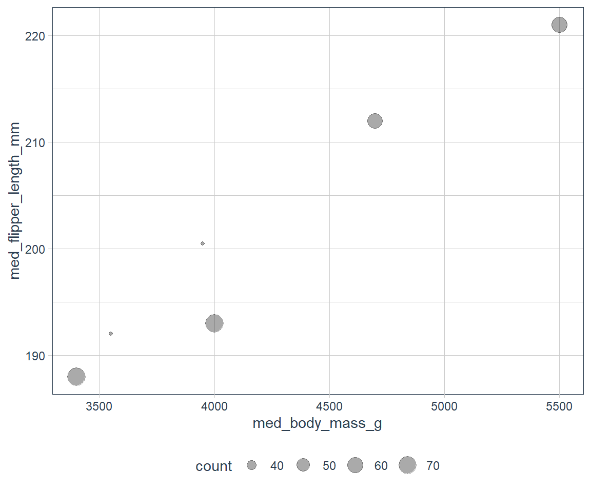
Using the pipe %>%
penguins %>%
  drop_na() %>%
  group_by(species, sex) %>%
  summarise(count = n(),
  med_bill_length_mm = median(bill_length_mm, na.rm = TRUE),
  med_bill_depth_mm = median(bill_depth_mm, na.rm = TRUE),
  med_flipper_length_mm = median(flipper_length_mm, na.rm = TRUE),
  med_body_mass_g = median(body_mass_g, na.rm = TRUE)) %>%
  ggplot(mapping = aes(x = med_body_mass_g,
                                      y = med_flipper_length_mm)) +
geom_point(aes(size = count), alpha = 1/3) 
Counts
n()which produces a count and,sum(is.na(some_variable))gives you the NA sum of data.
penguins %>%
  group_by(species) %>%
  summarise(count = n())
# A tibble: 3 x 2
species count
<fct> <int>
1 Adelie 152
2 Chinstrap 68
3 Gentoo 124# how many missing data in certain characteristics?
penguins %>%
select(species, body_mass_g) %>%
group_by(species) %>%
summarise(count = sum(is.na(body_mass_g)))# A tibble: 3 x 2
species count
<fct> <int>
1 Adelie 1
2 Chinstrap 0
3 Gentoo 1# how many missing data in certain characteristics?
penguins %>%
select(species, bill_length_mm) %>%
group_by(species) %>%
summarise(count = sum(is.na(bill_length_mm)))# A tibble: 3 x 2
species count
<fct> <int>
1 Adelie 1
2 Chinstrap 0
3 Gentoo 1Useful summary Functions
Measures of Location (mean, median etc.)
- Median: `median(x) is the value of x where 50% of the variable x lies above that value, and 50% of the variable x lies below that value.
not_cancelled <- flights %>%
  filter(!is.na(dep_delay),
         !is.na(arr_delay))

not_cancelled %>%
  group_by(year, month, day) %>%
  summarise(
    # avg_delay
    avg_delay1 = mean(arr_delay),
    # avg positive delay - filter our only positive arrival delay
    avg_delay2 = mean(arr_delay[arr_delay > 0])
  )
# A tibble: 365 x 5
# Groups: year, month [12]
year month day avg_delay1 avg_delay2
<int> <int> <int> <dbl> <dbl>
1 2013 1 1 12.7 32.5
2 2013 1 2 12.7 32.0
3 2013 1 3 5.73 27.7
4 2013 1 4 -1.93 28.3
5 2013 1 5 -1.53 22.6
6 2013 1 6 4.24 24.4
7 2013 1 7 -4.95 27.8
8 2013 1 8 -3.23 20.8
9 2013 1 9 -0.264 25.6
10 2013 1 10 -5.90 27.3
# ... with 355 more rowsMeasures of spread (sd, IQR etc.)
- Standard deviation: sd() measures the spread of a variable, the larger the sd the more dispersed the data.
- Inter Quartile Range: IQR() measures the spread in the middle - i.e. it measures the spread in the middle 50% of the variable. The measure is useful if there are outliers. \(IQR = Q{3} - Q{1}\).
- Median Absolute Deviation: mad() measures how far each point is from the median of the variable in absolute terms.
- Need the Mean Absolute Deviation: That can be found in the DescTools package.
not_cancelled %>%
  group_by(dest) %>%
  summarise(dist_sd = sd(distance),
            dist_iqr = IQR(distance),
            dist_mad = mad(distance)) %>%
  arrange(desc(dist_sd))
# A tibble: 104 x 4
dest dist_sd dist_iqr dist_mad
<chr> <dbl> <dbl> <dbl>
1 EGE 10.5 21 1.48
2 SAN 10.4 21 0
3 SFO 10.2 21 0
4 HNL 10.0 20 0
5 SEA 9.98 20 0
6 LAS 9.91 21 0
7 PDX 9.87 20 0
8 PHX 9.86 20 0
9 LAX 9.66 21 0
10 IND 9.46 20 0
# ... with 94 more rowsMeasures of rank - min() etc.
- min(), max(), quantile(x, 0.75)
- quantiles: quantile(x, 0.25) will find the value of x which is larger than 25% of the values, but less than the remaining 75%.
not_cancelled %>%
  group_by(year, month, day) %>%
  summarise(
    first = min(dep_time),
    last = max(dep_time)
  )
# A tibble: 365 x 5
# Groups: year, month [12]
year month day first last
<int> <int> <int> <int> <int>
1 2013 1 1 517 2356
2 2013 1 2 42 2354
3 2013 1 3 32 2349
4 2013 1 4 25 2358
5 2013 1 5 14 2357
6 2013 1 6 16 2355
7 2013 1 7 49 2359
8 2013 1 8 454 2351
9 2013 1 9 2 2252
10 2013 1 10 3 2320
# ... with 355 more rowsMeasures of position - first() etc.
- first() - i.e. x[1]
- nth(x, 2) - i.e. x[2]
- last(x) - i.e. x[length[x]]
- If the position does not exist, you may supply a default.
not_cancelled %>%
  group_by(year, month, day) %>%
  summarise(
    first = first(dep_time),
    last = last(dep_time)
  )
# A tibble: 365 x 5
# Groups: year, month [12]
year month day first last
<int> <int> <int> <int> <int>
1 2013 1 1 517 2356
2 2013 1 2 42 2354
3 2013 1 3 32 2349
4 2013 1 4 25 2358
5 2013 1 5 14 2357
6 2013 1 6 16 2355
7 2013 1 7 49 2359
8 2013 1 8 454 2351
9 2013 1 9 2 2252
10 2013 1 10 3 2320
# ... with 355 more rowsnot_cancelled %>%
group_by(year, month, day) %>%
# min_rank is like rank but for ties the method is min
mutate(r = min_rank(desc(dep_time))) %>%
filter(r %in% range(r))# A tibble: 770 x 20
# Groups: year, month, day [365]
year month day dep_time sched_dep_time dep_delay arr_time sched_arr_time
<int> <int> <int> <int> <int> <dbl> <int> <int>
1 2013 1 1 517 515 2 830 819
2 2013 1 1 2356 2359 -3 425 437
3 2013 1 2 42 2359 43 518 442
4 2013 1 2 2354 2359 -5 413 437
5 2013 1 3 32 2359 33 504 442
6 2013 1 3 2349 2359 -10 434 445
7 2013 1 4 25 2359 26 505 442
8 2013 1 4 2358 2359 -1 429 437
9 2013 1 4 2358 2359 -1 436 445
10 2013 1 5 14 2359 15 503 445
# ... with 760 more rows, and 12 more variables: arr_delay <dbl>,
# carrier <chr>, flight <int>, tailnum <chr>, origin <chr>, dest <chr>,
# air_time <dbl>, distance <dbl>, hour <dbl>, minute <dbl>, time_hour <dttm>,
# r <int>Counts
We have used n(), now we also have:
- count(x): raw counts in each category of x
- n_distinct(x): unique values in x
# Find distinct number of carriers at each dest
# and sort by highest to lowest
not_cancelled %>%
  group_by(dest) %>%
  summarise(num_carrier = n_distinct(carrier)) %>%
  arrange(desc(num_carrier))
# A tibble: 104 x 2
dest num_carrier
<chr> <int>
1 ATL 7
2 BOS 7
3 CLT 7
4 ORD 7
5 TPA 7
6 AUS 6
7 DCA 6
8 DTW 6
9 IAD 6
10 MSP 6
# ... with 94 more rows# counts are also useful
not_cancelled %>%
count(dest)# A tibble: 104 x 2
dest n
<chr> <int>
1 ABQ 254
2 ACK 264
3 ALB 418
4 ANC 8
5 ATL 16837
6 AUS 2411
7 AVL 261
8 BDL 412
9 BGR 358
10 BHM 269
# ... with 94 more rows# adding sort = TRUE puts the biggest counts at the top
not_cancelled %>%
count(dest, sort = TRUE)# A tibble: 104 x 2
dest n
<chr> <int>
1 ATL 16837
2 ORD 16566
3 LAX 16026
4 BOS 15022
5 MCO 13967
6 CLT 13674
7 SFO 13173
8 FLL 11897
9 MIA 11593
10 DCA 9111
# ... with 94 more rows# can add weighted counts
not_cancelled %>%
count(tailnum, wt = distance)# A tibble: 4,037 x 2
tailnum n
<chr> <dbl>
1 D942DN 3418
2 N0EGMQ 239143
3 N10156 109664
4 N102UW 25722
5 N103US 24619
6 N104UW 24616
7 N10575 139903
8 N105UW 23618
9 N107US 21677
10 N108UW 32070
# ... with 4,027 more rows# sum of logical values gives number of occurrences
# where something is TRUE
# How many flights were early, say before 5AM?
not_cancelled %>%
group_by(year, month, day) %>%
summarise(n_early = sum(dep_time < 500))# A tibble: 365 x 4
# Groups: year, month [12]
year month day n_early
<int> <int> <int> <int>
1 2013 1 1 0
2 2013 1 2 3
3 2013 1 3 4
4 2013 1 4 3
5 2013 1 5 3
6 2013 1 6 2
7 2013 1 7 2
8 2013 1 8 1
9 2013 1 9 3
10 2013 1 10 3
# ... with 355 more rows# mean of logical values gives a proportion
# how many flights were delayed more than an hour?
not_cancelled %>%
group_by(year, month, day) %>%
summarise(hour_prop = mean(arr_delay > 60))# A tibble: 365 x 4
# Groups: year, month [12]
year month day hour_prop
<int> <int> <int> <dbl>
1 2013 1 1 0.0722
2 2013 1 2 0.0851
3 2013 1 3 0.0567
4 2013 1 4 0.0396
5 2013 1 5 0.0349
6 2013 1 6 0.0470
7 2013 1 7 0.0333
8 2013 1 8 0.0213
9 2013 1 9 0.0202
10 2013 1 10 0.0183
# ... with 355 more rowsGrouping by Multiple Variables
When you group by multiple variables, each summary peels off one level of the grouping. It makes it easy to progressively roll up a dataset, but it should be used with sums and counts and not with medians etc.
daily <- group_by(flights, year, month, day)
# count flights per day
(per_day   <- summarise(daily, flights = n()))
# A tibble: 365 x 4
# Groups: year, month [12]
year month day flights
<int> <int> <int> <int>
1 2013 1 1 842
2 2013 1 2 943
3 2013 1 3 914
4 2013 1 4 915
5 2013 1 5 720
6 2013 1 6 832
7 2013 1 7 933
8 2013 1 8 899
9 2013 1 9 902
10 2013 1 10 932
# ... with 355 more rows# count flights per month
(per_month <- summarise(per_day, flights = sum(flights)))# A tibble: 12 x 3
# Groups: year [1]
year month flights
<int> <int> <int>
1 2013 1 27004
2 2013 2 24951
3 2013 3 28834
4 2013 4 28330
5 2013 5 28796
6 2013 6 28243
7 2013 7 29425
8 2013 8 29327
9 2013 9 27574
10 2013 10 28889
11 2013 11 27268
12 2013 12 28135# count flights per year
(per_year <- summarise(per_month, flights = sum(flights)))# A tibble: 1 x 2
year flights
<int> <int>
1 2013 336776Ungrouping
You can remove grouping as well.
daily %>%
  ungroup() %>%             # no longer grouped by date
  summarise(flights = n())  # count all flights
# A tibble: 1 x 1
flights
<int>
1 336776Exercises
Brainstorm at least 5 different ways to assess the typical delay characteristics of a group of flights. Consider the following scenarios:
A flight is 15 minutes early 50% of the time, and 15 minutes late 50% of the time.
A flight is always 10 minutes late.
A flight is 30 minutes early 50% of the time, and 30 minutes late 50% of the time.
99% of the time a flight is on time. 1% of the time it’s 2 hours late.
Which is more important: arrival delay or departure delay?
I think arrival delay is more important especially since many people have connecting flights. I would guess it would be more important in typical connection airports e.g. Atlanta, Los Angeles, international airports like Dubai, Qatar, Heathrow etc. as it is often an area which travellers pass through.
# The flights data has local flights within the US
flights %>%
  count(carrier, sort = TRUE)
# A tibble: 16 x 2 carrier n <chr> <int> 1 UA 58665 2 B6 54635 3 EV 54173 4 DL 48110 5 AA 32729 6 MQ 26397 7 US 20536 8 9E 18460 9 WN 12275 10 VX 5162 11 FL 3260 12 AS 714 13 F9 685 14 YV 601 15 HA 342 16 OO 32flights %>% count(dest, sort = TRUE)# A tibble: 105 x 2 dest n <chr> <int> 1 ORD 17283 2 ATL 17215 3 LAX 16174 4 BOS 15508 5 MCO 14082 6 CLT 14064 7 SFO 13331 8 FLL 12055 9 MIA 11728 10 DCA 9705 # ... with 95 more rows# Let's have a look at the busiest airports # It has changed a bit from our data of 2013 # https://en.wikipedia.org/wiki/List_of_the_busiest_airports_in_the_United_States flights %>% filter(dest %in% c('ATL', 'LAX', 'ORD', 'BOS', 'MCO')) %>% count(dest, sort = TRUE)# A tibble: 5 x 2 dest n <chr> <int> 1 ORD 17283 2 ATL 17215 3 LAX 16174 4 BOS 15508 5 MCO 14082top5_dests <- flights %>% add_count(dest, sort = TRUE, name = 'count') %>% select(dest, count) %>% count(dest, sort = TRUE) %>% slice_max(n, n = 5) top_dests <- flights %>% filter(dest %in% c(top5_dests %>% select(dest))$dest) top_dests %>% pivot_longer(cols = c(arr_delay, dep_delay), names_to = "metric", values_to = "value") %>% ggplot(aes(value, fill = dest)) + geom_density(alpha = 0.5) + facet_wrap(dest ~ metric, scales = "free", nrow = 3)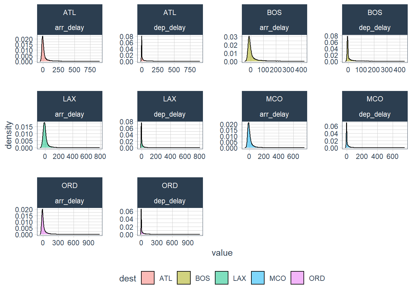
Come up with another approach that will give you the same output as
not_cancelled %>% count(dest)andnot_cancelled %>% count(tailnum, wt = distance)(without usingcount()).not_cancelled %>% count(dest)# A tibble: 104 x 2 dest n <chr> <int> 1 ABQ 254 2 ACK 264 3 ALB 418 4 ANC 8 5 ATL 16837 6 AUS 2411 7 AVL 261 8 BDL 412 9 BGR 358 10 BHM 269 # ... with 94 more rows# Alt: not_cancelled %>% group_by(dest) %>% summarise(n = n())# A tibble: 104 x 2 dest n <chr> <int> 1 ABQ 254 2 ACK 264 3 ALB 418 4 ANC 8 5 ATL 16837 6 AUS 2411 7 AVL 261 8 BDL 412 9 BGR 358 10 BHM 269 # ... with 94 more rowsnot_cancelled %>% count(tailnum, wt = distance)# A tibble: 4,037 x 2 tailnum n <chr> <dbl> 1 D942DN 3418 2 N0EGMQ 239143 3 N10156 109664 4 N102UW 25722 5 N103US 24619 6 N104UW 24616 7 N10575 139903 8 N105UW 23618 9 N107US 21677 10 N108UW 32070 # ... with 4,027 more rows# Alt: not_cancelled %>% group_by(tailnum) %>% summarise(n = sum(distance))# A tibble: 4,037 x 2 tailnum n <chr> <dbl> 1 D942DN 3418 2 N0EGMQ 239143 3 N10156 109664 4 N102UW 25722 5 N103US 24619 6 N104UW 24616 7 N10575 139903 8 N105UW 23618 9 N107US 21677 10 N108UW 32070 # ... with 4,027 more rowsOur definition of cancelled flights (
is.na(dep_delay) | is.na(arr_delay)) is slightly suboptimal. Why? Which is the most important column?On first thought I would assume that the dep_delay is most important since if it is null I would assume that is an indication of a cancellation.
# Okay let's look at the NAs in each column
flights %>%
  select(dep_delay, arr_delay, air_time) %>%
  summarise_all(~ sum(is.na(.)))
# A tibble: 1 x 3 dep_delay arr_delay air_time <int> <int> <int> 1 8255 9430 9430Okay, so the arr_delay count of NAs is larger and is the same as the NULLs in air_time. What could be the reason for arr_delay NULLs being larger than dep_delay NULLs? One could be crashes but there does not seem to be crashes from flights originating out of NY. The other could be diverted flights. I therefore think we need to have a definition of what is considered cancelled? If diversions are considered cancelled then the arr_delay being NULL is more important, if diversions are not included the dep_delay being NULL should be considered. Without talking to an aviation expert I looked at a wikipedia page that seems to suggest that cancellations are that the airline does not operate the flight at all for a certain reason
Look at the number of cancelled flights per day. Is there a pattern? Is the proportion of cancelled flights related to the average delay?
# Keeping to the definition of cancellations being either # true non-flights and diversions cancelled <- flights %>% filter(is.na(dep_delay) | is.na(arr_delay)) cancelled <- cancelled %>% group_by(year, month, day) %>% summarise(num_cancelled = n()) avg_delays <- flights %>% group_by(year, month, day) %>% summarise(num_flights_on_day = n(), avg_dep_delay = mean(dep_delay[dep_delay > 0], na.rm = TRUE), avg_arr_delay = mean(arr_delay[arr_delay > 0], na.rm = TRUE)) # we haven't seen this yet but this joins the two datasets # so we can analyse it # For now consider inner_join as tagging on columns for avg_delays onto # cancelled where the cancelled.year = avg_delays.year, # cancelled.month = avg_delays.month and cancelled.day = avg_delays.day cancelled %>% inner_join(avg_delays) %>% # here again we use a function that we have not seen yet # we make a date using the {lubridate} from the # components of the date - year, month, day mutate(date = make_date(year, month, day), prop_cancelled = num_cancelled / num_flights_on_day) %>% pivot_longer(cols = c(num_cancelled, prop_cancelled, num_flights_on_day, avg_dep_delay, avg_arr_delay), names_to = "metric", values_to = "value") %>% ggplot(aes(x = date, y = value, fill = metric)) + geom_point() + labs(title = "Number of delayed flights and the average delay on the day", y = "Measure of Metric") + facet_wrap(~ metric, scales = "free_y") + geom_smooth(se = FALSE)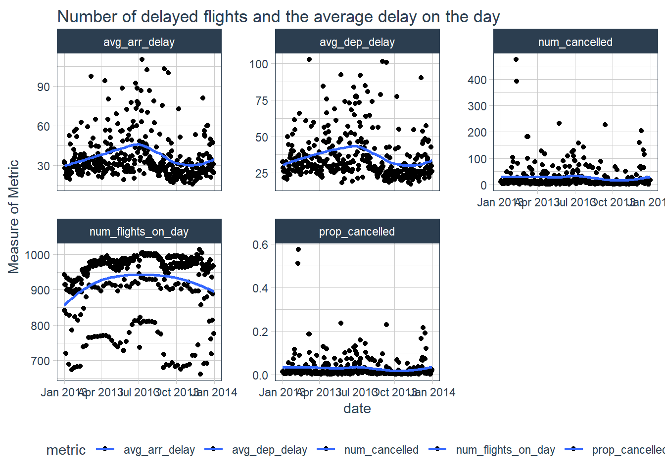 If you look at the proportion of cancelled flights it does seem as though this increases the average delays experienced.
Which carrier has the worst delays?
flights %>%
  mutate(avg_delay = mean(dep_delay, na.rm=TRUE)) %>%
  group_by(carrier) %>%
  mutate(avg_delay_carrier = mean(dep_delay, na.rm = TRUE)) %>%
  select(carrier, avg_delay, avg_delay_carrier) %>%
  distinct() %>%
  filter(avg_delay_carrier > avg_delay) %>%
  arrange(-avg_delay_carrier)
# A tibble: 8 x 3 # Groups: carrier [8] carrier avg_delay avg_delay_carrier <chr> <dbl> <dbl> 1 F9 12.6 20.2 2 EV 12.6 20.0 3 YV 12.6 19.0 4 FL 12.6 18.7 5 WN 12.6 17.7 6 9E 12.6 16.7 7 B6 12.6 13.0 8 VX 12.6 12.9flights %>% mutate(avg_arr_delay = mean(arr_delay, na.rm=TRUE)) %>% group_by(carrier) %>% mutate(avg_arr_delay_carrier = mean(arr_delay, na.rm = TRUE)) %>% select(carrier, avg_arr_delay, avg_arr_delay_carrier) %>% distinct() %>% filter(avg_arr_delay_carrier > avg_arr_delay) %>% arrange(-avg_arr_delay_carrier)# A tibble: 9 x 3 # Groups: carrier [9] carrier avg_arr_delay avg_arr_delay_carrier <chr> <dbl> <dbl> 1 F9 6.90 21.9 2 FL 6.90 20.1 3 EV 6.90 15.8 4 YV 6.90 15.6 5 OO 6.90 11.9 6 MQ 6.90 10.8 7 WN 6.90 9.65 8 B6 6.90 9.46 9 9E 6.90 7.38Challenge: can you disentangle the effects of bad airports vs. bad carriers? Why/why not? (Hint: think about
flights %>% group_by(carrier, dest) %>% summarise(n()))flights %>% group_by(carrier, dest) %>% summarise(n())# A tibble: 314 x 3 # Groups: carrier [16] carrier dest `n()` <chr> <chr> <int> 1 9E ATL 59 2 9E AUS 2 3 9E AVL 10 4 9E BGR 1 5 9E BNA 474 6 9E BOS 914 7 9E BTV 2 8 9E BUF 833 9 9E BWI 856 10 9E CAE 3 # ... with 304 more rows# 3 origins flights %>% count(origin, sort = TRUE)# A tibble: 3 x 2 origin n <chr> <int> 1 EWR 120835 2 JFK 111279 3 LGA 104662# many destinations flights %>% count(dest, sort = TRUE)# A tibble: 105 x 2 dest n <chr> <int> 1 ORD 17283 2 ATL 17215 3 LAX 16174 4 BOS 15508 5 MCO 14082 6 CLT 14064 7 SFO 13331 8 FLL 12055 9 MIA 11728 10 DCA 9705 # ... with 95 more rows# how many carriers flights %>% count(carrier, sort = TRUE)# A tibble: 16 x 2 carrier n <chr> <int> 1 UA 58665 2 B6 54635 3 EV 54173 4 DL 48110 5 AA 32729 6 MQ 26397 7 US 20536 8 9E 18460 9 WN 12275 10 VX 5162 11 FL 3260 12 AS 714 13 F9 685 14 YV 601 15 HA 342 16 OO 32flights %>% count(carrier, dest, sort = TRUE) %>% slice_max(n = 25, order_by = n) %>% gt()carrier dest n DL ATL 10571 US CLT 8632 AA DFW 7257 AA MIA 7234 UA ORD 6984 UA IAH 6924 UA SFO 6819 B6 FLL 6563 B6 MCO 6472 AA ORD 6059 UA LAX 5823 MQ RDU 4794 US DCA 4716 B6 BOS 4383 US BOS 4283 WN MDW 4113 EV IAD 4048 DL DTW 3875 UA DEN 3796 DL MCO 3663 AA LAX 3582 UA BOS 3342 UA MCO 3217 B6 PBI 3161 DL MIA 2929 # how many combos of carrier and dest? (dests <- flights %>% distinct(carrier, dest))# A tibble: 314 x 2 carrier dest <chr> <chr> 1 UA IAH 2 AA MIA 3 B6 BQN 4 DL ATL 5 UA ORD 6 B6 FLL 7 EV IAD 8 B6 MCO 9 AA ORD 10 B6 PBI # ... with 304 more rows# notice every carrier does not fly to every destination across_all <- flights %>% mutate(avg_arr_delay = mean(arr_delay[arr_delay>0], na.rm = TRUE), med_arr_delay = median(arr_delay[arr_delay>0], na.rm = TRUE)) %>% group_by(carrier) %>% mutate(avg_carrier_arr_delay = mean(arr_delay[arr_delay>0], na.rm = TRUE), med_carrier_arr_delay = median(arr_delay[arr_delay>0], na.rm = TRUE)) %>% ungroup() %>% group_by(dest) %>% mutate(avg_dest_arr_delay = mean(arr_delay[arr_delay>0], na.rm = TRUE), med_dest_arr_delay = median(arr_delay[arr_delay>0], na.rm = TRUE)) %>% ungroup() %>% group_by(carrier, dest) %>% mutate(avg_cd_arr_delay = mean(arr_delay[arr_delay>0], na.rm = TRUE), med_cd_arr_delay = median(arr_delay[arr_delay>0], na.rm = TRUE)) %>% ungroup() %>% select(carrier, dest, avg_arr_delay, avg_carrier_arr_delay, avg_dest_arr_delay, avg_cd_arr_delay, med_arr_delay, med_carrier_arr_delay, med_dest_arr_delay, med_cd_arr_delay) %>% arrange(desc(avg_cd_arr_delay), -med_cd_arr_delay) %>% distinct() across_all%>% head(25) %>% gt()carrier dest avg_arr_delay avg_carrier_arr_delay avg_dest_arr_delay avg_cd_arr_delay med_arr_delay med_carrier_arr_delay med_dest_arr_delay med_cd_arr_delay UA STL 40.3425 36.65098 43.73392 242.00000 21 19.0 22.0 242.0 OO DTW 40.3425 60.60000 42.44949 157.00000 21 47.0 21.0 157.0 OO ORD 40.3425 60.60000 45.66731 107.00000 21 47.0 24.0 107.0 EV TVC 40.3425 48.26858 66.68571 77.47619 21 28.0 40.0 40.0 EV TYS 40.3425 48.26858 59.86645 72.63819 21 28.0 39.0 57.0 YV CLT 40.3425 51.08140 35.53289 65.89474 21 27.5 18.0 49.0 9E ROC 40.3425 49.27271 48.98307 65.37363 21 27.0 29.0 29.0 WN MSY 40.3425 40.74755 43.09886 62.46429 21 19.0 22.0 30.5 DL SAT 40.3425 37.74356 52.32296 62.14159 21 17.0 30.0 34.0 EV DSM 40.3425 48.26858 57.02692 61.81193 21 28.0 35.5 41.0 EV TUL 40.3425 48.26858 60.37306 60.37306 21 28.0 43.0 43.0 EV BHM 40.3425 48.26858 60.05785 60.05785 21 28.0 44.0 44.0 VX SFO 40.3425 43.84708 41.57175 60.03035 21 17.0 21.0 26.5 EV CLE 40.3425 48.26858 43.97520 58.68584 21 28.0 23.0 36.0 MQ ORF 40.3425 37.85205 47.67700 58.61594 21 20.0 29.0 39.5 DL PIT 40.3425 37.74356 42.55926 56.56471 21 17.0 23.0 28.0 EV OKC 40.3425 48.26858 56.56219 56.56219 21 28.0 42.0 42.0 UA RDU 40.3425 36.65098 39.88509 56.00000 21 19.0 21.0 56.0 9E ORD 40.3425 49.27271 45.66731 55.49299 21 27.0 24.0 34.0 EV ROC 40.3425 48.26858 48.98307 55.47682 21 28.0 29.0 30.0 9E MCI 40.3425 49.27271 49.31729 55.15873 21 27.0 30.5 33.5 9E CVG 40.3425 49.27271 52.37917 55.07014 21 27.0 29.0 32.0 9E CAE 40.3425 49.27271 53.63218 55.00000 21 27.0 36.0 55.0 9E CLE 40.3425 49.27271 43.97520 54.54971 21 27.0 23.0 31.0 9E BWI 40.3425 49.27271 50.92793 54.49013 21 27.0 29.0 30.0 across_all %>% count(carrier, sort = TRUE)# A tibble: 16 x 2 carrier n <chr> <int> 1 EV 61 2 9E 49 3 UA 47 4 B6 42 5 DL 40 6 MQ 20 7 AA 19 8 WN 11 9 US 6 10 OO 5 11 VX 5 12 FL 3 13 YV 3 14 AS 1 15 F9 1 16 HA 1across_all %>% count(dest, sort=TRUE)# A tibble: 105 x 2 dest n <chr> <int> 1 ATL 7 2 BOS 7 3 CLT 7 4 ORD 7 5 TPA 7 6 AUS 6 7 DCA 6 8 DTW 6 9 IAD 6 10 MSP 6 # ... with 95 more rowsacross_all_dep <- flights %>% mutate(avg_dep_delay = mean(dep_delay[dep_delay>0], na.rm = TRUE), med_dep_delay = median(dep_delay[dep_delay>0], na.rm = TRUE)) %>% group_by(carrier) %>% mutate(avg_carrier_dep_delay = mean(dep_delay[dep_delay>0], na.rm = TRUE), med_carrier_dep_delay = median(dep_delay[dep_delay>0], na.rm = TRUE)) %>% ungroup() %>% group_by(origin) %>% mutate(avg_dest_dep_delay = mean(dep_delay[dep_delay>0], na.rm = TRUE), med_dest_dep_delay = median(dep_delay[dep_delay>0], na.rm = TRUE)) %>% ungroup() %>% group_by(carrier, origin) %>% mutate(avg_cd_dep_delay = mean(dep_delay[dep_delay>0], na.rm = TRUE), med_cd_dep_delay = median(dep_delay[dep_delay>0], na.rm = TRUE)) %>% ungroup() %>% select(carrier, origin, avg_dep_delay, avg_carrier_dep_delay, avg_dest_dep_delay, avg_cd_dep_delay, med_dep_delay, med_carrier_dep_delay, med_dest_dep_delay, med_cd_dep_delay) %>% arrange(desc(avg_cd_dep_delay), -med_cd_dep_delay) %>% distinct() across_all_dep %>% head(25) %>% gt()carrier origin avg_dep_delay avg_carrier_dep_delay avg_dest_dep_delay avg_cd_dep_delay med_dep_delay med_carrier_dep_delay med_dest_dep_delay med_cd_dep_delay OO LGA 39.37323 58.00000 41.63096 62.33333 19 40 20 53.5 EV JFK 39.37323 50.32979 38.04677 56.79497 19 31 18 25.0 EV LGA 39.37323 50.32979 41.63096 55.40676 19 31 20 35.0 YV LGA 39.37323 52.95279 41.63096 52.95279 19 30 20 30.0 MQ EWR 39.37323 44.91533 38.98792 52.21845 19 27 19 32.5 9E JFK 39.37323 48.92001 38.04677 49.63199 19 27 18 27.0 OO EWR 39.37323 58.00000 38.98792 49.33333 19 40 19 13.0 EV EWR 39.37323 50.32979 38.98792 49.27670 19 31 19 30.0 DL EWR 39.37323 37.40024 38.98792 48.57807 19 16 19 20.0 B6 EWR 39.37323 39.79422 38.98792 48.20826 19 21 19 24.0 B6 LGA 39.37323 39.79422 41.63096 47.98956 19 21 20 23.0 9E EWR 39.37323 48.92001 38.98792 47.76404 19 27 19 27.0 AA EWR 39.37323 37.16926 38.98792 47.18388 19 16 19 22.0 MQ JFK 39.37323 44.91533 38.04677 45.77984 19 27 18 25.5 F9 LGA 39.37323 45.13783 41.63096 45.13783 19 18 20 18.0 HA JFK 39.37323 44.84058 38.04677 44.84058 19 5 18 5.0 9E LGA 39.37323 48.92001 41.63096 43.34028 19 27 20 26.0 MQ LGA 39.37323 44.91533 41.63096 43.21583 19 27 20 27.0 VX EWR 39.37323 34.45483 38.98792 42.06239 19 10 19 13.0 DL LGA 39.37323 37.40024 41.63096 41.01359 19 16 20 18.0 FL LGA 39.37323 40.82588 41.63096 40.82588 19 16 20 16.0 UA LGA 39.37323 29.92619 41.63096 38.38985 19 12 20 15.0 AA LGA 39.37323 37.16926 41.63096 37.98608 19 16 20 17.0 B6 JFK 39.37323 39.79422 38.04677 37.54221 19 21 18 20.0 WN EWR 39.37323 34.85743 38.98792 35.42240 19 15 19 16.0 across_all_dep %>% count(carrier, sort = TRUE)# A tibble: 16 x 2 carrier n <chr> <int> 1 9E 3 2 AA 3 3 B6 3 4 DL 3 5 EV 3 6 MQ 3 7 UA 3 8 US 3 9 OO 2 10 VX 2 11 WN 2 12 AS 1 13 F9 1 14 FL 1 15 HA 1 16 YV 1across_all_dep %>% count(origin, sort=TRUE)# A tibble: 3 x 2 origin n <chr> <int> 1 LGA 13 2 EWR 12 3 JFK 10There does seem more of a delay based on carrier than on airport but I can’t put much faith in this since I did not do a thorough investigation - for example some carriers had more flights, some destinations are busier. We should therefore look at proportions of all flights maybe, and there are other specifics that I as an aviation newbie have not even thought of. Here I had a rough look at the average and median delay by carrier, destination and the combination of carrier and destination. Sorting by the largest delays in the combination average and median gets us to seeming a lot of delays from particular carriers like EV, but I wouldn’t put much faith in this until a proper investigation is done.
For each plane, count the number of flights before the first delay of greater than 1 hour.
# Dep delay flights %>% # group by plane group_by(tailnum) %>% # arrange by flight date arrange(year, month, day) %>% # assign a row number to each mutate(row_number = row_number()) %>% # ungroup to clear the grouping ungroup() %>% # okay get only the delays beyond 60 min filter(dep_delay > 60) %>% # group again by plane group_by(tailnum) %>% # the number of flights before the first delay will be the # row number - 1 mutate(num_flights = first(row_number) - 1) %>% select(tailnum, num_flights) %>% distinct() %>% arrange(desc(num_flights)) %>% DT::datatable()# Let's check one of them to ensure we're on the right track flights %>% filter(tailnum == 'N712TW') %>% select(year, month, day, tailnum, dep_delay) %>% arrange(year, month, day) %>% DT::datatable()# Arrival delays flights %>% # group by plane group_by(tailnum) %>% # arrange by flight date arrange(year, month, day) %>% # assign a row number to each mutate(row_number = row_number()) %>% # ungroup to clear the grouping ungroup() %>% # okay get only the delays beyond 60 min filter(arr_delay > 60) %>% # group again by plane group_by(tailnum) %>% # the number of flights before the first delay will be the # row number - 1 mutate(num_flights = first(row_number) - 1) %>% select(tailnum, num_flights) %>% distinct() %>% filter(num_flights > 25) %>% arrange(num_flights, tailnum) %>% DT::datatable()# Let's check one of them to ensure we're on the right track # It's on Page 16 in the DT above, entry 152 flights %>% filter(tailnum == 'N597UA') %>% select(year, month, day, tailnum, arr_delay) %>% arrange(year, month, day) %>% DT::datatable()What does the
sortargument tocount()do. When might you use it?The
sort = TRUEin count() allows us to see the items with the highest counts up at the top - it sorts the count in descending order.
Exercises
Refer back to the lists of useful mutate and filtering functions. Describe how each operation changes when you combine it with grouping.
When you combine a mutate with a group it depends on the function you use within the mutate. Above I used a row_number to mark each row in a set. In the case above I considered each plane (tailnum) as a separate group and wanted to know how many flights before that plane had a delay of above 60 min. The authors note that grouped mutates work best with window functions like
lagorlead, it also works alright with mean(), median() etc. where it first creates the group then gets the aggregate value for that variable for the group. We often do this in SQL but I think in R this is equivalent to thesummarise()function.SELECT dest , AVG(arr_delay) -- Average arrival delay FROM flights WHERE arr_delay > 0 GROUP BY destWe can also do arithmetic using
+,-, etc. but this is not affected by the group and hence grouping does not make sense.Which plane (
tailnum) has the worst on-time record?# okay one way may be to see who from a pure # count has the most flights with arrival delays flights %>% filter(!is.na(tailnum), !is.na(arr_delay), arr_delay > 0) %>% select(tailnum, arr_delay) %>% count(tailnum, sort = TRUE)# A tibble: 3,874 x 2 tailnum n <chr> <int> 1 N725MQ 215 2 N228JB 192 3 N258JB 191 4 N713MQ 185 5 N711MQ 184 6 N723MQ 180 7 N531MQ 174 8 N190JB 173 9 N353JB 173 10 N534MQ 172 # ... with 3,864 more rows# BUT the above is not really useful, I mean it does # not consider how many flights did that plane do etc. # So let's consider that. flights %>% add_count(tailnum, name = 'num_flights_plane') %>% filter(!is.na(tailnum), !is.na(arr_delay), arr_delay > 0) %>% select(tailnum, arr_delay, num_flights_plane) %>% filter(num_flights_plane > 10) %>% # some planes had few flights add_count(tailnum, name = 'num_delayed') %>% mutate(prop_delayed = num_delayed / num_flights_plane) %>% select(tailnum, num_flights_plane, num_delayed, prop_delayed) %>% distinct() %>% arrange(desc(prop_delayed))# A tibble: 3,399 x 4 tailnum num_flights_plane num_delayed prop_delayed <chr> <int> <int> <dbl> 1 N337AT 13 12 0.923 2 N169AT 11 10 0.909 3 N168AT 18 16 0.889 4 N290AT 16 14 0.875 5 N273AT 13 11 0.846 6 N913JB 16 13 0.812 7 N326AT 18 14 0.778 8 N988AT 37 28 0.757 9 N673UA 16 12 0.75 10 N983AT 32 24 0.75 # ... with 3,389 more rowsflights %>% filter(tailnum %in% c('N337AT', 'N169AT', 'N988AT')) %>% select(year, month, day, tailnum, arr_delay) %>% arrange(tailnum) %>% DT::datatable()# We can also probably look at the total number of minutes # each plane has as arr_delay vs the total arr_delay minutes # overall for all delayed flights flights %>% filter(!is.na(tailnum), !is.na(arr_delay), arr_delay > 0) %>% select(tailnum, arr_delay) %>% mutate(tot_delay = sum(arr_delay)) %>% group_by(tailnum) %>% mutate(plane_delay = sum(arr_delay), prop_delay = plane_delay / tot_delay) %>% ungroup() %>% select(tailnum, plane_delay, tot_delay, prop_delay) %>% distinct() %>% arrange(desc(prop_delay))# A tibble: 3,874 x 4 tailnum plane_delay tot_delay prop_delay <chr> <dbl> <dbl> <dbl> 1 N228JB 8861 5365714 0.00165 2 N15980 8770 5365714 0.00163 3 N15910 8737 5365714 0.00163 4 N258JB 8234 5365714 0.00153 5 N192JB 8025 5365714 0.00150 6 N16919 7955 5365714 0.00148 7 N292JB 7680 5365714 0.00143 8 N10575 7412 5365714 0.00138 9 N725MQ 7274 5365714 0.00136 10 N324JB 7264 5365714 0.00135 # ... with 3,864 more rows# Checks for one plane flights %>% filter(!is.na(tailnum), !is.na(arr_delay), arr_delay > 0) %>% summarise(sum(arr_delay))# A tibble: 1 x 1 `sum(arr_delay)` <dbl> 1 5365714flights %>% filter(!is.na(arr_delay), arr_delay > 0, tailnum == 'N228JB') %>% summarise(sum(arr_delay))# A tibble: 1 x 1 `sum(arr_delay)` <dbl> 1 8861What time of day should you fly if you want to avoid delays as much as possible?
# there's often times where there is a departure delay but # the time is made up in flight, so I am going to consider # arr_delay only flights %>% select(sched_dep_time, arr_delay) %>% filter(!is.na(arr_delay)) %>% group_by(sched_dep_time) %>% mutate(total_arr_delay = sum(arr_delay)) %>% select(sched_dep_time, total_arr_delay) %>% distinct() %>% arrange(total_arr_delay)# A tibble: 1,020 x 2 # Groups: sched_dep_time [1,020] sched_dep_time total_arr_delay <int> <dbl> 1 700 -30362 2 600 -19958 3 730 -19621 4 800 -18150 5 630 -17364 6 900 -12779 7 725 -8097 8 945 -7149 9 915 -7138 10 745 -6327 # ... with 1,010 more rowsThe best time is at 7h00 but truly you’re pretty good to go if you depart between 6h00 - 8h00 😁
For each destination, compute the total minutes of delay. For each flight, compute the proportion of the total delay for its destination.
flights %>% # Let's first get only those flights which were late filter(arr_delay > 0) %>% group_by(dest) %>% # Let's get the total delay for each dest mutate(tot_delay = sum(arr_delay, na.rm = TRUE)) %>% ungroup() %>% group_by(year, month, day, tailnum) %>% mutate(flight_delay_prop = arr_delay / tot_delay) %>% # select a subset of cols of interest to us select(year, month, day, tailnum, dest, arr_delay, tot_delay, flight_delay_prop) %>% # sort by descending flight_delay_prop arrange(-flight_delay_prop)# A tibble: 133,004 x 8 # Groups: year, month, day, tailnum [113,364] year month day tailnum dest arr_delay tot_delay flight_delay_prop <int> <int> <int> <chr> <chr> <dbl> <dbl> <dbl> 1 2013 8 17 N528UA ANC 39 62 0.629 2 2013 3 30 N806UA MTJ 101 170 0.594 3 2013 3 16 N839VA PSP 17 36 0.472 4 2013 11 22 N398CA SBN 53 125 0.424 5 2013 11 1 N761ND SBN 50 125 0.4 6 2013 3 16 N817UA HDN 43 119 0.361 7 2013 12 28 N436UA BZN 154 491 0.314 8 2013 12 25 N16701 JAC 175 619 0.283 9 2013 12 21 N474UA HDN 32 119 0.269 10 2013 3 8 N611QX CHO 228 947 0.241 # ... with 132,994 more rowsDelays are typically temporally correlated: even once the problem that caused the initial delay has been resolved, later flights are delayed to allow earlier flights to leave. Using
lag(), explore how the delay of a flight is related to the delay of the immediately preceding flight.flights_sub <- flights %>% filter(dep_delay > 0) %>% arrange(year, month, day, origin, dep_time) %>% group_by(year, month, day, origin) %>% mutate(prev_delay = lag(dep_delay)) %>% filter(dep_delay > 0, prev_delay > 0) %>% select(year, month, day, origin, tailnum, dep_time, dep_delay, prev_delay) %>% arrange(year, month, day, origin, dep_time) flights_sub %>% slice_head(n = 50) %>% DT::datatable()flights_sub %>% ggplot(aes(prev_delay, dep_delay, colour = origin)) + geom_point() + geom_smooth(se = FALSE) + scale_colour_tq()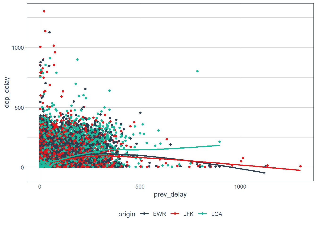
Departure delay does seem to increase with the previous delay, if we look at flights leaving a destination in particular. This just considers what flights leave airport X on a particular day. Irrespective of carrier, or actual plane we then see what’s the delay of flight 2 in comparison to the previous flights delay. It increases up to a point and then gets better. I took out negative delays so this may be a nonsensical way of looking at flight delays as a consequence of previous flight delays. Plus we have a time element here that we’re not addressing! So it’s hard to understand anything from this to be honest.
What if we keep negative delays in, and just looked at a period of the data?
flights_sub <- flights %>% filter(!is.na(dep_delay), !is.na(arr_delay) # take out cancelled flights ) %>% arrange(year, month, day, origin, dep_time) %>% group_by(year, month, day, origin) %>% mutate(prev_delay = lag(dep_delay)) %>% filter(!is.na(dep_delay), !is.na(prev_delay)) %>% select(year, month, day, origin, tailnum, dep_time, dep_delay, prev_delay) %>% arrange(year, month, day, origin, dep_time) %>% filter(month == 1, day %in% c(1:12)) flights_sub %>% slice_head(n = 50) %>% DT::datatable()flights_sub %>% arrange(year, month, day, origin, dep_time) %>% ggplot(aes(prev_delay, dep_delay, colour = origin)) + geom_point() + geom_smooth(se = FALSE) + scale_colour_tq() + facet_wrap(~ day, nrow = 4) + labs(title = "How does the current delay stack up against the previous delay?", caption = "Data for first 12 days in January")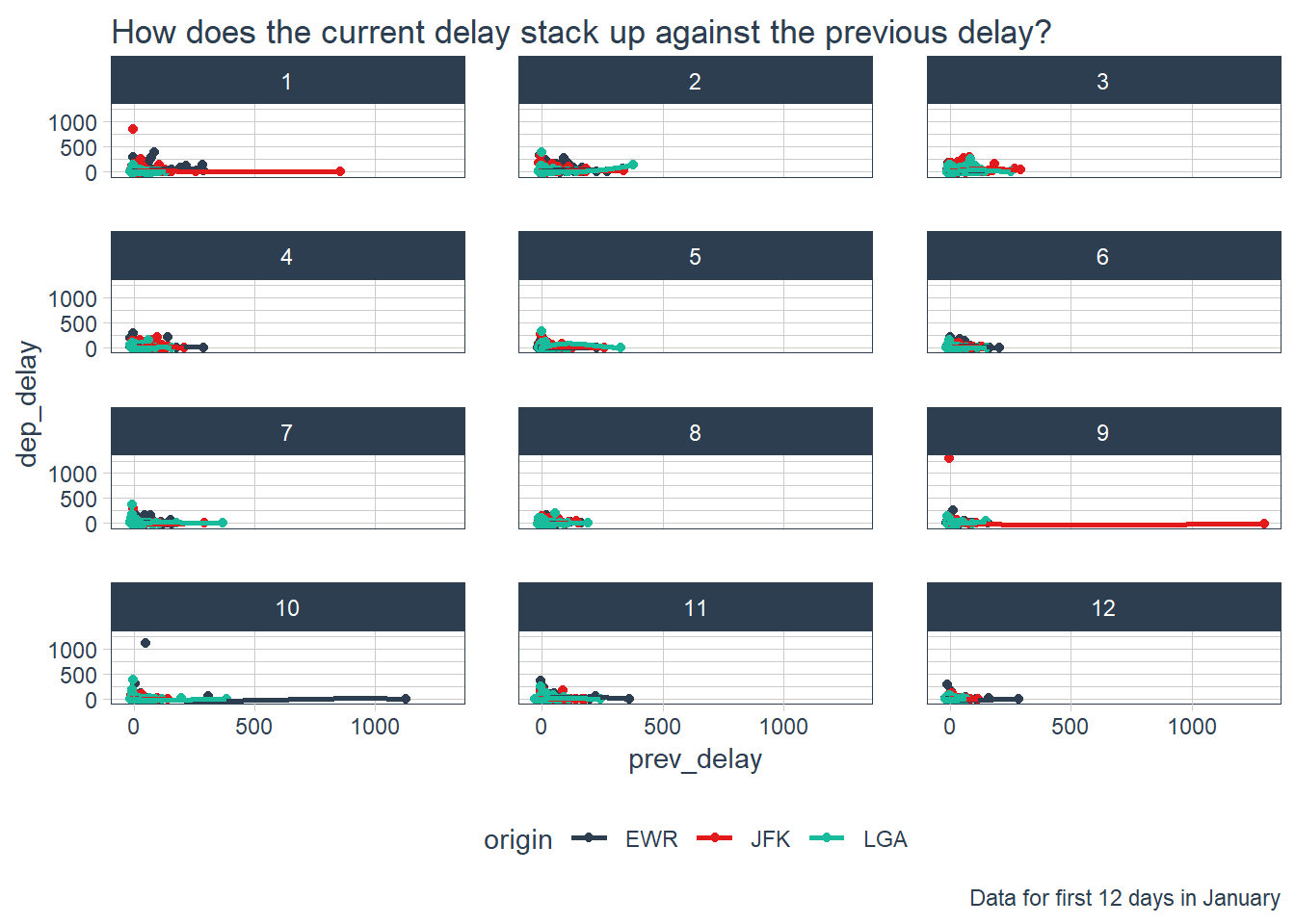
flights_sub2 <- flights %>% filter(!is.na(dep_delay), !is.na(arr_delay) # take out cancelled flights ) %>% arrange(year, month, day, origin, dep_time) %>% group_by(year, month, day, origin) %>% mutate(prev_delay = lag(dep_delay)) %>% filter(!is.na(dep_delay), !is.na(prev_delay)) %>% select(year, month, day, origin, tailnum, dep_time, dep_delay, prev_delay) %>% arrange(year, month, day, origin, dep_time) %>% filter(month == 11, day %in% c(10:22)) flights_sub2 %>% arrange(year, month, day, origin, dep_time) %>% ggplot(aes(prev_delay, dep_delay, colour = origin)) + geom_point() + geom_smooth(se = FALSE) + scale_colour_tq() + facet_wrap(~ day, nrow = 4) + labs(title = "How does the current delay stack up against the previous delay?", caption = "Data for 10-22 of November")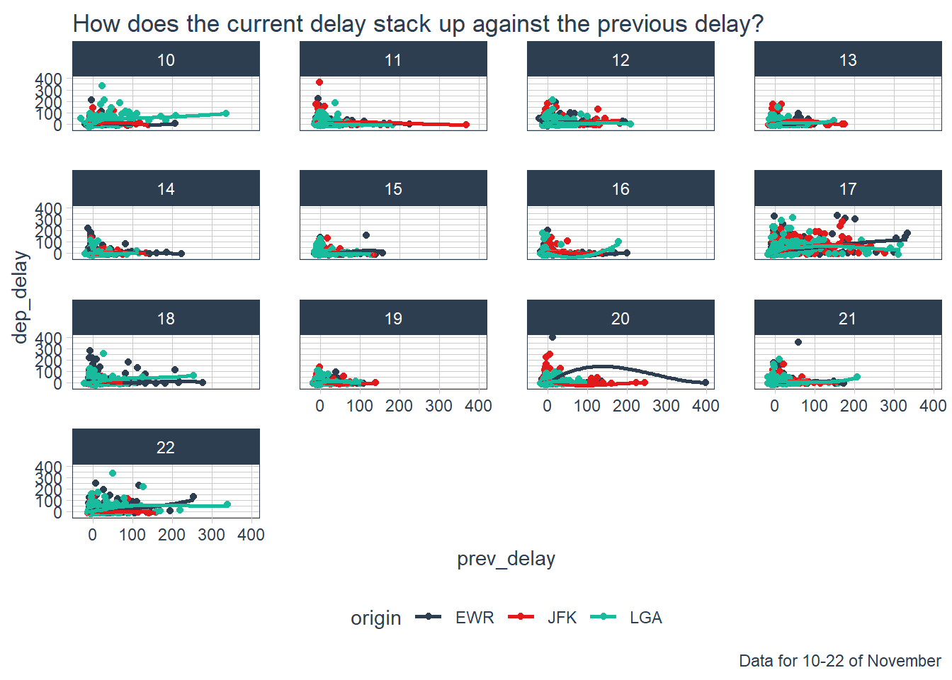
It still shows recovery for quite a few origin airports, so the airport and carrier make strides in rectifying delays. Maybe the ahead of schedule and late also kind of cancel each other out?
What about if we consider the particular carrier delays? Does a carrier delay have a knock on effect on their other flights?
flights_sub <- flights %>% filter(!is.na(dep_delay), !is.na(arr_delay) # take out cancelled flights ) %>% arrange(year, month, day, origin, carrier, dep_time) %>% group_by(year, month, day, origin, carrier) %>% mutate(prev_delay = lag(dep_delay)) %>% filter(!is.na(dep_delay), !is.na(prev_delay)) %>% select(year, month, day, origin, carrier, dep_time, dep_delay, prev_delay) %>% arrange(year, month, day, origin, carrier, dep_time) %>% filter(month == 1, day %in% c(1:12)) flights_sub %>% slice_head(n = 50) %>% DT::datatable()flights_sub %>% arrange(year, month, day, origin, carrier, dep_time) %>% ggplot(aes(prev_delay, dep_delay, colour = carrier)) + geom_point() + geom_smooth(se = FALSE) + scale_colour_tq() + facet_wrap(~ day, nrow = 4) + labs(title = "How does the current delay stack up against the previous delay?", caption = "Data for first 12 days in January")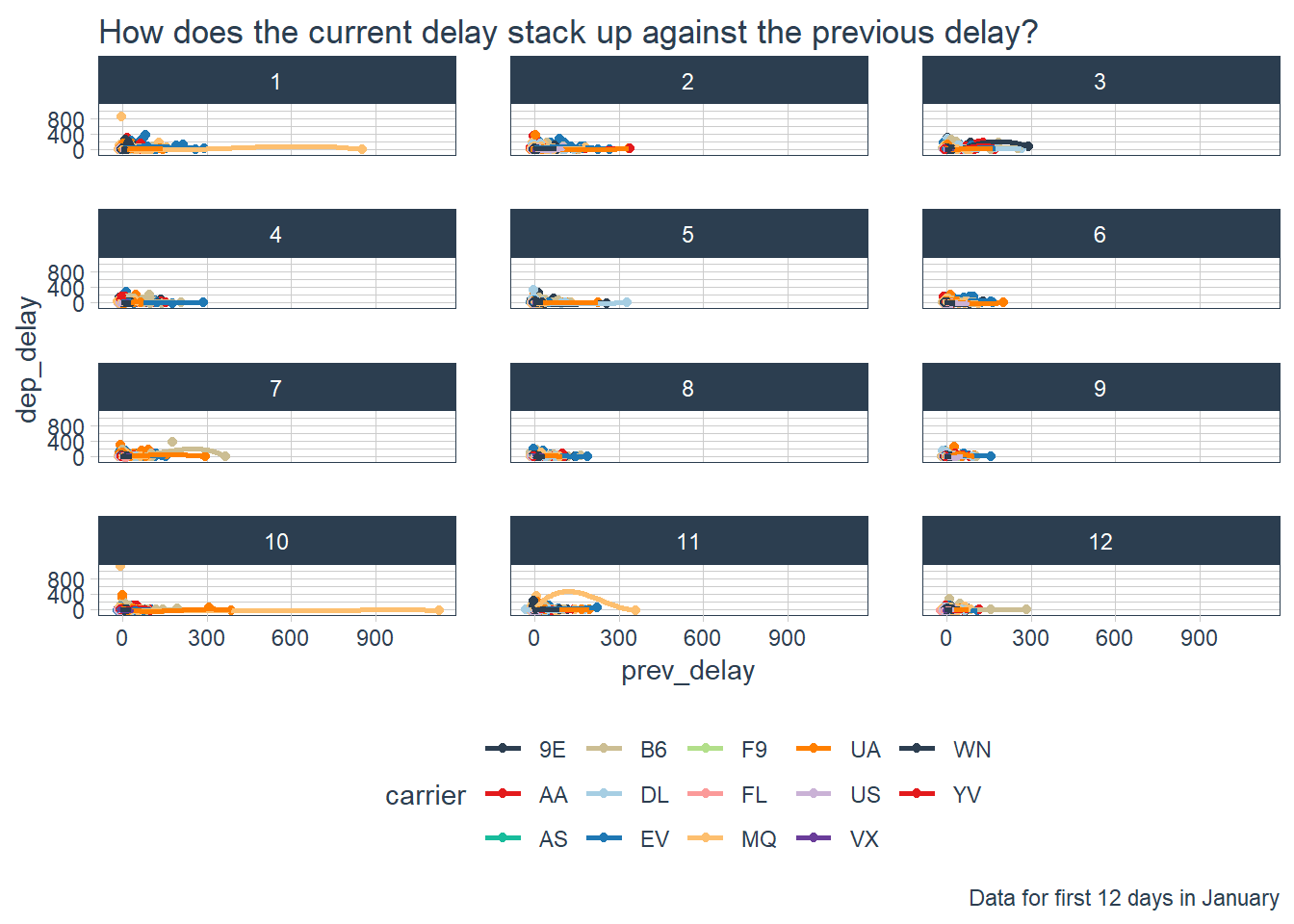
Okay we could spend an entire day looking at the data to be considerate here. For the purposes of answering the exercise question it does seem that delays increase as a result of previous delays indicating there may be some knock on effect during the day. The pattern rectifies itself over the course of the day it seems, but I must be honest I did a cursory check here so I’d rather give conclusions after more analysis.
Look at each destination. Can you find flights that are suspiciously fast? (i.e. flights that represent a potential data entry error). Compute the air time of a flight relative to the shortest flight to that destination. Which flights were most delayed in the air?
flights %>% filter(air_time > 0) %>% arrange(air_time) %>% select(year, month, day, origin, dest, dep_delay, arr_delay, air_time)# A tibble: 327,346 x 8 year month day origin dest dep_delay arr_delay air_time <int> <int> <int> <chr> <chr> <dbl> <dbl> <dbl> 1 2013 1 16 EWR BDL 40 31 20 2 2013 4 13 EWR BDL 10 -6 20 3 2013 12 6 EWR BDL 31 27 21 4 2013 2 3 EWR PHL 24 23 21 5 2013 2 5 EWR BDL -12 -29 21 6 2013 2 12 EWR PHL -7 -14 21 7 2013 3 2 LGA BOS -10 -21 21 8 2013 3 8 JFK PHL 51 35 21 9 2013 3 18 EWR BDL 87 67 21 10 2013 3 19 EWR BDL 41 19 21 # ... with 327,336 more rowsflight_stats <- flights %>% filter(air_time > 0) %>% group_by(origin, dest) %>% mutate(mean_time_to_dest = mean(air_time, na.rm = TRUE), median_time_to_dest = median(air_time, na.rm = TRUE), sd = sd(air_time, na.rm = TRUE), diff = air_time - median_time_to_dest) %>% select(origin, dest, air_time, mean_time_to_dest, median_time_to_dest, sd, diff) %>% arrange((diff)) # suspiciously quick airtime flight_stats %>% head(10) %>% gt()air_time mean_time_to_dest median_time_to_dest sd diff EWR - MSP 93 150.8102 149 11.95731 -56 EWR - SNA 274 329.2894 329 19.88961 -55 279 329.2894 329 19.88961 -50 279 329.2894 329 19.88961 -50 JFK - LAX 275 329.1511 329 18.17139 -54 277 329.1511 329 18.17139 -52 279 329.1511 329 18.17139 -50 280 329.1511 329 18.17139 -49 JFK - SEA 275 329.3745 328 15.30094 -53 EWR - HNL 562 612.0752 611 21.26614 -49 # most time in air flight_stats %>% tail(10) %>% gt()air_time mean_time_to_dest median_time_to_dest sd diff EWR - AUS 301 211.24765 210 17.908306 91 JFK - LAX 422 329.15109 329 18.171386 93 440 329.15109 329 18.171386 111 EWR - OKC 284 193.00952 190 19.307846 94 286 193.00952 190 19.307846 96 JFK - ACK 141 42.06818 41 8.127495 100 EWR - LAS 399 299.03869 298 17.145578 101 LGA - DEN 331 227.51600 227 15.436637 104 JFK - EGE 382 256.44554 255 18.658765 127 JFK - SFO 490 347.40363 347 16.852680 143 Find all destinations that are flown by at least two carriers. Use that information to rank the carriers.
flights %>% group_by(dest) %>% # for each dest mutate(num_carriers = n_distinct(carrier)) %>% # count number carriers ungroup() %>% filter(num_carriers > 1) %>% # we want destinations having 2+ carriers group_by(carrier) %>% # for each carrier summarise(num_dests = n_distinct(dest)) %>% # count number destinations arrange(-num_dests) # put carrier flying to biggest #destinations at top# A tibble: 16 x 2 carrier num_dests <chr> <int> 1 EV 51 2 9E 48 3 UA 42 4 DL 39 5 B6 35 6 AA 19 7 MQ 19 8 WN 10 9 OO 5 10 US 5 11 VX 4 12 YV 3 13 FL 2 14 AS 1 15 F9 1 16 HA 1
sessionInfo()R version 3.6.3 (2020-02-29)
Platform: x86_64-w64-mingw32/x64 (64-bit)
Running under: Windows 10 x64 (build 18363)
Matrix products: default
locale:
[1] LC_COLLATE=English_South Africa.1252 LC_CTYPE=English_South Africa.1252
[3] LC_MONETARY=English_South Africa.1252 LC_NUMERIC=C
[5] LC_TIME=English_South Africa.1252
attached base packages:
[1] stats graphics grDevices utils datasets methods base
other attached packages:
[1] magrittr_1.5 tidyquant_1.0.0
[3] quantmod_0.4.17 TTR_0.23-6
[5] PerformanceAnalytics_2.0.4 xts_0.12-0
[7] zoo_1.8-7 lubridate_1.7.8
[9] emo_0.0.0.9000 skimr_2.1.1
[11] gt_0.2.2 palmerpenguins_0.1.0
[13] nycflights13_1.0.1 flair_0.0.2
[15] forcats_0.5.0 stringr_1.4.0
[17] dplyr_1.0.0 purrr_0.3.4
[19] readr_1.3.1 tidyr_1.1.0
[21] tibble_3.0.3 ggplot2_3.3.0
[23] tidyverse_1.3.0 workflowr_1.6.2
loaded via a namespace (and not attached):
[1] nlme_3.1-144 fs_1.4.1 httr_1.4.2 rprojroot_1.3-2
[5] repr_1.1.0 tools_3.6.3 backports_1.1.6 DT_0.13
[9] utf8_1.1.4 R6_2.4.1 DBI_1.1.0 mgcv_1.8-31
[13] colorspace_1.4-1 withr_2.2.0 tidyselect_1.1.0 curl_4.3
[17] compiler_3.6.3 git2r_0.26.1 cli_2.0.2 rvest_0.3.5
[21] xml2_1.3.2 labeling_0.3 sass_0.2.0 scales_1.1.0
[25] checkmate_2.0.0 quadprog_1.5-8 digest_0.6.25 rmarkdown_2.4
[29] base64enc_0.1-3 pkgconfig_2.0.3 htmltools_0.5.0 dbplyr_1.4.3
[33] highr_0.8 htmlwidgets_1.5.1 rlang_0.4.7 readxl_1.3.1
[37] rstudioapi_0.11 generics_0.0.2 farver_2.0.3 jsonlite_1.7.0
[41] crosstalk_1.1.0.1 Matrix_1.2-18 Rcpp_1.0.4.6 Quandl_2.10.0
[45] munsell_0.5.0 fansi_0.4.1 lifecycle_0.2.0 stringi_1.4.6
[49] whisker_0.4 yaml_2.2.1 grid_3.6.3 promises_1.1.0
[53] crayon_1.3.4 lattice_0.20-38 haven_2.2.0 splines_3.6.3
[57] hms_0.5.3 knitr_1.28 pillar_1.4.6 reprex_0.3.0
[61] glue_1.4.1 evaluate_0.14 modelr_0.1.6 vctrs_0.3.2
[65] httpuv_1.5.2 cellranger_1.1.0 gtable_0.3.0 assertthat_0.2.1
[69] xfun_0.13 broom_0.5.6 later_1.0.0 ellipsis_0.3.1