Pre- and post-fire anaylisis of soils by Fire date
Last updated: 2021-09-14
Checks: 7 0
Knit directory: soil_alcontar/
This reproducible R Markdown analysis was created with workflowr (version 1.6.2). The Checks tab describes the reproducibility checks that were applied when the results were created. The Past versions tab lists the development history.
Great! Since the R Markdown file has been committed to the Git repository, you know the exact version of the code that produced these results.
Great job! The global environment was empty. Objects defined in the global environment can affect the analysis in your R Markdown file in unknown ways. For reproduciblity it’s best to always run the code in an empty environment.
The command set.seed(20210907) was run prior to running the code in the R Markdown file. Setting a seed ensures that any results that rely on randomness, e.g. subsampling or permutations, are reproducible.
Great job! Recording the operating system, R version, and package versions is critical for reproducibility.
Nice! There were no cached chunks for this analysis, so you can be confident that you successfully produced the results during this run.
Great job! Using relative paths to the files within your workflowr project makes it easier to run your code on other machines.
Great! You are using Git for version control. Tracking code development and connecting the code version to the results is critical for reproducibility.
The results in this page were generated with repository version 56e0949. See the Past versions tab to see a history of the changes made to the R Markdown and HTML files.
Note that you need to be careful to ensure that all relevant files for the analysis have been committed to Git prior to generating the results (you can use wflow_publish or wflow_git_commit). workflowr only checks the R Markdown file, but you know if there are other scripts or data files that it depends on. Below is the status of the Git repository when the results were generated:
Ignored files:
    Ignored:    .RData
    Ignored:    .Rhistory
    Ignored:    .Rproj.user/C369E4F4/
    Ignored:    .Rproj.user/shared/notebooks/0EF54E14-NOBORRAR/
    Ignored:    .Rproj.user/shared/notebooks/27FF967E-analysis_pre_post_epoca/
    Ignored:    .Rproj.user/shared/notebooks/33E25F73-analysis_resilience/
    Ignored:    .Rproj.user/shared/notebooks/3F603CAC-map/
    Ignored:    .Rproj.user/shared/notebooks/4672E36C-study_area/
    Ignored:    .Rproj.user/shared/notebooks/4A68381F-general_overview_soils/
    Ignored:    .Rproj.user/shared/notebooks/4E13660A-temporal_comparison/
    Ignored:    .Rproj.user/shared/notebooks/5D919DFD-analysis_zona_time_postFire/
    Ignored:    .Rproj.user/shared/notebooks/827D0727-analysis_pre_post/
    Ignored:    .Rproj.user/shared/notebooks/A3F813C2-index/
    Ignored:    .Rproj.user/shared/notebooks/D4E3AA10-analysis_zona_time/

Untracked files:
    Untracked:  analysis/NOBORRAR.Rmd
    Untracked:  analysis/analysis_pre_post_cache/
    Untracked:  analysis/test.Rmd
    Untracked:  data/spatial/01_EP_ANDALUCIA/EP_Andalucía.shp.DESKTOP-CKNNEUJ.5492.5304.sr.lock
    Untracked:  data/spatial/lucdeme/
    Untracked:  data/spatial/parcelas/GEO_PARCELAS.shp.DESKTOP-CKNNEUJ.5492.5304.sr.lock
    Untracked:  data/spatial/test/
    Untracked:  map.Rmd
    Untracked:  output/anovas_pre_post_epoca.csv
    Untracked:  output/anovas_zona_time.csv
    Untracked:  output/anovas_zona_time_postFire.csv
    Untracked:  scripts/generate_3dview.R

Unstaged changes:
    Modified:   analysis/_site.yml
    Modified:   analysis/analysis_zona_time_postFire.Rmd
    Modified:   data/spatial/.DS_Store
    Modified:   data/spatial/01_EP_ANDALUCIA/EP_Andalucía.dbf
    Deleted:    index.Rmd
    Modified:   scripts/00_prepare_data.R
    Modified:   temporal_comparison.Rmd
Note that any generated files, e.g. HTML, png, CSS, etc., are not included in this status report because it is ok for generated content to have uncommitted changes.
These are the previous versions of the repository in which changes were made to the R Markdown (analysis/analysis_pre_post_epoca.Rmd) and HTML (docs/analysis_pre_post_epoca.html) files. If you’ve configured a remote Git repository (see ?wflow_git_remote), click on the hyperlinks in the table below to view the files as they were in that past version.
| File | Version | Author | Date | Message |
|---|---|---|---|---|
| Rmd | 56e0949 | ajpelu | 2021-09-14 | change fechaQuema por estacion; momento por |
| html | 389b963 | ajpelu | 2021-09-14 | Build site. |
| Rmd | 9ba7a9d | ajpelu | 2021-09-14 | add analysis by date Fire |
Prepare data
raw_soil <- readxl::read_excel(here::here("data/Resultados_Suelos_2018_2021_v2.xlsx"),
    sheet = "SEGUIMIENTO_SUELOS_sin_ouliers") %>% janitor::clean_names() %>% mutate(treatment_name = case_when(str_detect(geo_parcela_nombre,
    "NP_") ~ "Autumn Burning / No Browsing", str_detect(geo_parcela_nombre, "PR_") ~
    "Spring Burning / Browsing", str_detect(geo_parcela_nombre, "P_") ~ "Autumn Burning / Browsing"),
    zona = case_when(str_detect(geo_parcela_nombre, "NP_") ~ "QOt_NP", str_detect(geo_parcela_nombre,
        "PR_") ~ "QPr_P", str_detect(geo_parcela_nombre, "P_") ~ "QOt_P"), estacion = case_when(str_detect(geo_parcela_nombre,
        "NP_") ~ "Ot", str_detect(geo_parcela_nombre, "PR_") ~ "Pr", str_detect(geo_parcela_nombre,
        "P_") ~ "Ot"), date = lubridate::ymd(fecha), fecha = case_when(pre_post_quema ==
"Prequema" ~ "0 preQuema", pre_post_quema == "Postquema" ~ "1 postQuema"))- Select data pre- and intermediately post-fire (first post-fire sampling: “2018-12-20” and “2019-05-09” for autumn and spring fires respectively)
soil <- raw_soil %>% filter(date %in% lubridate::ymd(c("2018-12-11", "2018-12-20",
"2019-04-24", "2019-05-09"))) %>% mutate(zona = as.factor(zona), fecha = as.factor(fecha))- Structure of the data
             estacion
fecha         Ot Pr
  0 preQuema  48 24
  1 postQuema 48 24
Modelize
- For each response variable, the approach modelling is
\(Y \sim estacion (Ot|Pr) + fecha(pre|post) + estacion \times fecha\)
using the “(1|estacion:geo_parcela_nombre)” as nested random effects
Then explore error distribution of the variable response and model diagnostics
Select the appropiate error distribution and use LMM or GLMM
Explore Post-hoc
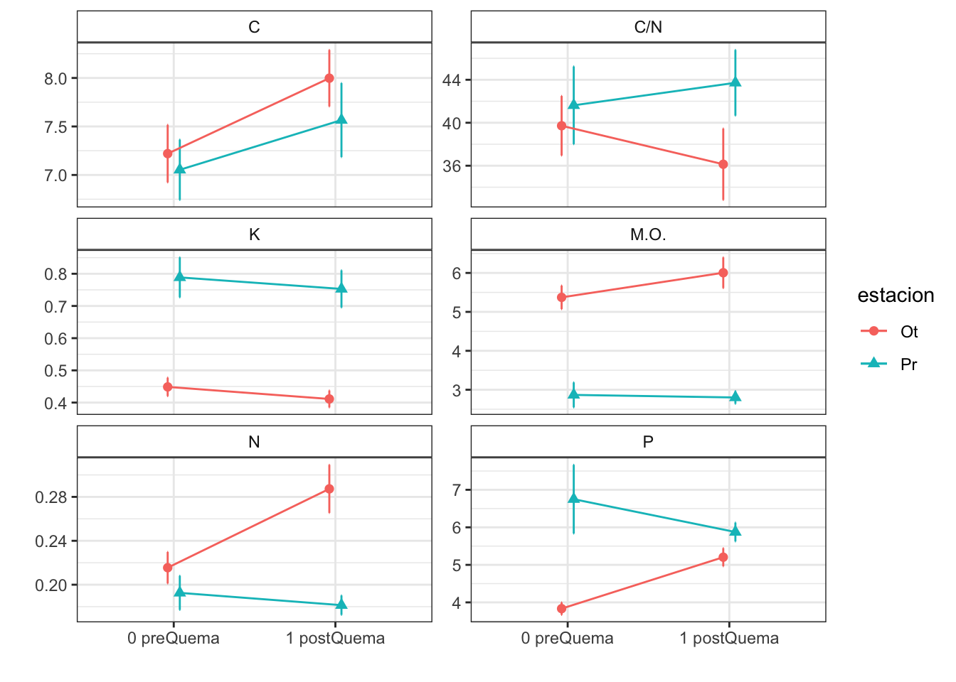
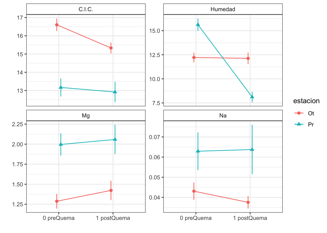
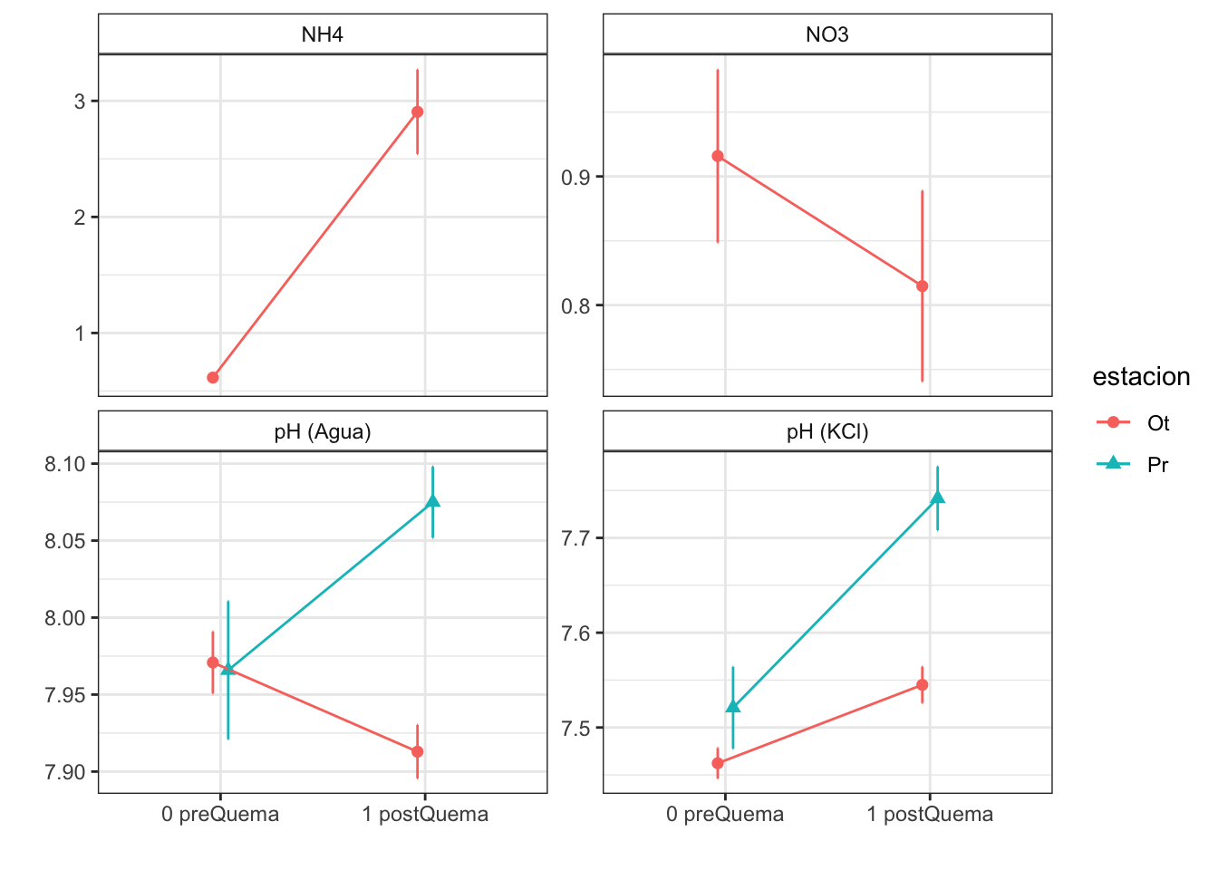
Plot interactions
Humedad
Model
Type III Analysis of Variance Table with Satterthwaite's method
               Sum Sq Mean Sq NumDF DenDF F value    Pr(>F)
fecha          461.74  461.74     1   130 50.4197 7.257e-11 ***
estacion         0.53    0.53     1    10  0.0575    0.8153
fecha:estacion 439.95  439.95     1   130 48.0407 1.748e-10 ***
---
Signif. codes:  0 '***' 0.001 '**' 0.01 '*' 0.05 '.' 0.1 ' ' 1
Sum Sq Mean Sq NumDF DenDF F value Pr(>F)
fecha 461.7404592 461.7404592 1 130 50.41969020 7.256505e-11
estacion 0.5268064 0.5268064 1 10 0.05752456 8.152969e-01
fecha:estacion 439.9539281 439.9539281 1 130 48.04071273 1.748462e-10
variable factor
fecha humedad fecha
estacion humedad estacion
fecha:estacion humedad fecha:estacionPost-hoc
$`emmeans of fecha`
 fecha       emmean    SE   df lower.CL upper.CL
 0 preQuema    13.9 0.689 13.8    12.44     15.4
 1 postQuema   10.1 0.689 13.8     8.64     11.6

Results are averaged over the levels of: estacion
Degrees-of-freedom method: kenward-roger
Confidence level used: 0.95

$`pairwise differences of fecha`
 1                        estimate    SE  df t.ratio p.value
 0 preQuema - 1 postQuema      3.8 0.535 130 7.101   <.0001

Results are averaged over the levels of: estacion
Degrees-of-freedom method: kenward-roger
$`emmeans of estacion`
estacion emmean SE df lower.CL upper.CL
Ot 12.2 0.734 10 10.54 13.8
Pr 11.9 1.038 10 9.56 14.2
Results are averaged over the levels of: fecha
Degrees-of-freedom method: kenward-roger
Confidence level used: 0.95
$`pairwise differences of estacion`
1 estimate SE df t.ratio p.value
Ot - Pr 0.305 1.27 10 0.240 0.8153
Results are averaged over the levels of: fecha
Degrees-of-freedom method: kenward-roger $`emmeans of fecha | estacion`
estacion = Ot:
fecha emmean SE df lower.CL upper.CL
0 preQuema 12.22 0.796 13.8 10.5 13.9
1 postQuema 12.13 0.796 13.8 10.4 13.8
estacion = Pr:
fecha emmean SE df lower.CL upper.CL
0 preQuema 15.62 1.126 13.8 13.2 18.0
1 postQuema 8.11 1.126 13.8 5.7 10.5
Degrees-of-freedom method: kenward-roger
Confidence level used: 0.95
$`pairwise differences of fecha | estacion`
estacion = Ot:
2 estimate SE df t.ratio p.value
0 preQuema - 1 postQuema 0.0907 0.618 130 0.147 0.8835
estacion = Pr:
2 estimate SE df t.ratio p.value
0 preQuema - 1 postQuema 7.5065 0.874 130 8.593 <.0001
Degrees-of-freedom method: kenward-roger CIC
Model
Type III Analysis of Variance Table with Satterthwaite's method
               Sum Sq Mean Sq NumDF DenDF F value  Pr(>F)
fecha          18.503  18.503     1   130  5.1118 0.02543 *
estacion       35.605  35.605     1    10  9.8361 0.01058 *
fecha:estacion  8.337   8.337     1   130  2.3031 0.13154
---
Signif. codes:  0 '***' 0.001 '**' 0.01 '*' 0.05 '.' 0.1 ' ' 1
Sum Sq Mean Sq NumDF DenDF F value Pr(>F)
fecha 18.503472 18.503472 1 130.000001 5.111751 0.02542616
estacion 35.604511 35.604511 1 9.999998 9.836067 0.01057742
fecha:estacion 8.336806 8.336806 1 130.000001 2.303118 0.13154272
variable factor
fecha cic fecha
estacion cic estacion
fecha:estacion cic fecha:estacionPost-hoc
$`emmeans of fecha`
 fecha       emmean    SE   df lower.CL upper.CL
 0 preQuema    14.9 0.496 12.8     13.8     16.0
 1 postQuema   14.1 0.496 12.8     13.1     15.2

Results are averaged over the levels of: estacion
Degrees-of-freedom method: kenward-roger
Confidence level used: 0.95

$`pairwise differences of fecha`
 1                        estimate    SE  df t.ratio p.value
 0 preQuema - 1 postQuema     0.76 0.336 130 2.261   0.0254

Results are averaged over the levels of: estacion
Degrees-of-freedom method: kenward-roger
$`emmeans of estacion`
estacion emmean SE df lower.CL upper.CL
Ot 16 0.539 10 14.8 17.2
Pr 13 0.762 10 11.3 14.7
Results are averaged over the levels of: fecha
Degrees-of-freedom method: kenward-roger
Confidence level used: 0.95
$`pairwise differences of estacion`
1 estimate SE df t.ratio p.value
Ot - Pr 2.93 0.933 10 3.136 0.0106
Results are averaged over the levels of: fecha
Degrees-of-freedom method: kenward-roger $`emmeans of fecha | estacion`
estacion = Ot:
fecha emmean SE df lower.CL upper.CL
0 preQuema 16.6 0.573 12.8 15.4 17.8
1 postQuema 15.3 0.573 12.8 14.1 16.6
estacion = Pr:
fecha emmean SE df lower.CL upper.CL
0 preQuema 13.2 0.810 12.8 11.4 14.9
1 postQuema 12.9 0.810 12.8 11.2 14.7
Degrees-of-freedom method: kenward-roger
Confidence level used: 0.95
$`pairwise differences of fecha | estacion`
estacion = Ot:
2 estimate SE df t.ratio p.value
0 preQuema - 1 postQuema 1.27 0.388 130 3.272 0.0014
estacion = Pr:
2 estimate SE df t.ratio p.value
0 preQuema - 1 postQuema 0.25 0.549 130 0.455 0.6497
Degrees-of-freedom method: kenward-roger C
Model
Type III Analysis of Variance Table with Satterthwaite's method
                Sum Sq Mean Sq NumDF DenDF F value  Pr(>F)
fecha          13.3214 13.3214     1   130  6.1796 0.01419 *
estacion        0.2542  0.2542     1    10  0.1179 0.73843
fecha:estacion  0.5636  0.5636     1   130  0.2614 0.61001
---
Signif. codes:  0 '***' 0.001 '**' 0.01 '*' 0.05 '.' 0.1 ' ' 1
Sum Sq Mean Sq NumDF DenDF F value Pr(>F)
fecha 13.3214014 13.3214014 1 130.000000 6.1795805 0.01419189
estacion 0.2541669 0.2541669 1 9.999999 0.1179039 0.73842869
fecha:estacion 0.5635681 0.5635681 1 130.000000 0.2614300 0.61000674
variable factor
fecha c_percent fecha
estacion c_percent estacion
fecha:estacion c_percent fecha:estacionPost-hoc
$`emmeans of fecha`
 fecha       emmean    SE   df lower.CL upper.CL
 0 preQuema    7.14 0.455 11.8     6.14     8.13
 1 postQuema   7.78 0.455 11.8     6.79     8.77

Results are averaged over the levels of: estacion
Degrees-of-freedom method: kenward-roger
Confidence level used: 0.95

$`pairwise differences of fecha`
 1                        estimate   SE  df t.ratio p.value
 0 preQuema - 1 postQuema   -0.645 0.26 130 -2.486  0.0142

Results are averaged over the levels of: estacion
Degrees-of-freedom method: kenward-roger
$`emmeans of estacion`
estacion emmean SE df lower.CL upper.CL
Ot 7.61 0.503 10 6.49 8.73
Pr 7.31 0.712 10 5.72 8.90
Results are averaged over the levels of: fecha
Degrees-of-freedom method: kenward-roger
Confidence level used: 0.95
$`pairwise differences of estacion`
1 estimate SE df t.ratio p.value
Ot - Pr 0.299 0.872 10 0.343 0.7384
Results are averaged over the levels of: fecha
Degrees-of-freedom method: kenward-roger $`emmeans of fecha | estacion`
estacion = Ot:
fecha emmean SE df lower.CL upper.CL
0 preQuema 7.22 0.525 11.8 6.07 8.37
1 postQuema 8.00 0.525 11.8 6.85 9.14
estacion = Pr:
fecha emmean SE df lower.CL upper.CL
0 preQuema 7.05 0.743 11.8 5.43 8.67
1 postQuema 7.57 0.743 11.8 5.95 9.19
Degrees-of-freedom method: kenward-roger
Confidence level used: 0.95
$`pairwise differences of fecha | estacion`
estacion = Ot:
2 estimate SE df t.ratio p.value
0 preQuema - 1 postQuema -0.778 0.300 130 -2.596 0.0105
estacion = Pr:
2 estimate SE df t.ratio p.value
0 preQuema - 1 postQuema -0.512 0.424 130 -1.209 0.2288
Degrees-of-freedom method: kenward-roger Fe
Model
Fitting one lmer() model. [DONE]
Calculating p-values. [DONE]
Mixed Model Anova Table (Type 3 tests, KR-method)
Model: fe_percent ~ fecha * estacion + (1 | estacion:geo_parcela_nombre)
Data: df_model
Effect df F p.value
1 fecha 1, 130 0.28 .598
2 estacion 1, 10 0.46 .512
3 fecha:estacion 1, 130 0.21 .648
---
Signif. codes: 0 '***' 0.001 '**' 0.01 '*' 0.05 '+' 0.1 ' ' 1Fitting one lmer() model. [DONE]
Calculating p-values. [DONE]Mixed Model Anova Table (Type 3 tests, KR-method)
Model: fe_percent ~ fecha * estacion + (1 | estacion:geo_parcela_nombre)
Data: df_model
num Df den Df F Pr(>F)
fecha 1 130 0.2796 0.5979
estacion 1 10 0.4631 0.5116
fecha:estacion 1 130 0.2093 0.6481Post-hoc
$`emmeans of fecha`
fecha emmean SE df asymp.LCL asymp.UCL
0 preQuema 0.545 0.036 Inf 0.475 0.616
1 postQuema 0.554 0.036 Inf 0.484 0.625
Results are averaged over the levels of: estacion
Results are given on the inverse (not the response) scale.
Confidence level used: 0.95
$`pairwise differences of fecha`
1 estimate SE df z.ratio p.value
0 preQuema - 1 postQuema -0.00898 0.0167 Inf -0.539 0.5898
Results are averaged over the levels of: estacion
Note: contrasts are still on the inverse scale $`emmeans of estacion`
estacion emmean SE df asymp.LCL asymp.UCL
Ot 0.568 0.0398 Inf 0.490 0.646
Pr 0.532 0.0573 Inf 0.419 0.644
Results are averaged over the levels of: fecha
Results are given on the inverse (not the response) scale.
Confidence level used: 0.95
$`pairwise differences of estacion`
1 estimate SE df z.ratio p.value
Ot - Pr 0.0364 0.0695 Inf 0.524 0.6006
Results are averaged over the levels of: fecha
Note: contrasts are still on the inverse scale $`emmeans of fecha | estacion`
estacion = Ot:
fecha emmean SE df asymp.LCL asymp.UCL
0 preQuema 0.559 0.0410 Inf 0.479 0.640
1 postQuema 0.576 0.0411 Inf 0.496 0.657
estacion = Pr:
fecha emmean SE df asymp.LCL asymp.UCL
0 preQuema 0.531 0.0588 Inf 0.416 0.646
1 postQuema 0.532 0.0588 Inf 0.417 0.647
Results are given on the inverse (not the response) scale.
Confidence level used: 0.95
$`pairwise differences of fecha | estacion`
estacion = Ot:
2 estimate SE df z.ratio p.value
0 preQuema - 1 postQuema -0.01688 0.0200 Inf -0.843 0.3991
estacion = Pr:
2 estimate SE df z.ratio p.value
0 preQuema - 1 postQuema -0.00109 0.0266 Inf -0.041 0.9675
Note: contrasts are still on the inverse scale MO
Model
Fitting one lmer() model. [DONE]
Calculating p-values. [DONE]
Mixed Model Anova Table (Type 3 tests, KR-method)
Model: mo ~ fecha * estacion + (1 | estacion:geo_parcela_nombre)
Data: df_model
Effect df F p.value
1 fecha 1, 130 0.60 .439
2 estacion 1, 10 35.18 *** <.001
3 fecha:estacion 1, 130 0.91 .341
---
Signif. codes: 0 '***' 0.001 '**' 0.01 '*' 0.05 '+' 0.1 ' ' 1Fitting one lmer() model. [DONE]
Calculating p-values. [DONE]Mixed Model Anova Table (Type 3 tests, KR-method)
Model: mo ~ fecha * estacion + (1 | estacion:geo_parcela_nombre)
Data: df_model
num Df den Df F Pr(>F)
fecha 1 130 0.6020 0.4392419
estacion 1 10 35.1850 0.0001448 ***
fecha:estacion 1 130 0.9143 0.3407472
---
Signif. codes: 0 '***' 0.001 '**' 0.01 '*' 0.05 '.' 0.1 ' ' 1Post-hoc
$`emmeans of fecha`
fecha emmean SE df asymp.LCL asymp.UCL
0 preQuema 0.271 0.0190 Inf 0.233 0.308
1 postQuema 0.265 0.0191 Inf 0.228 0.302
Results are averaged over the levels of: estacion
Results are given on the inverse (not the response) scale.
Confidence level used: 0.95
$`pairwise differences of fecha`
1 estimate SE df z.ratio p.value
0 preQuema - 1 postQuema 0.00557 0.0229 Inf 0.243 0.8082
Results are averaged over the levels of: estacion
Note: contrasts are still on the inverse scale $`emmeans of estacion`
estacion emmean SE df asymp.LCL asymp.UCL
Ot 0.181 0.0143 Inf 0.153 0.209
Pr 0.355 0.0265 Inf 0.303 0.407
Results are averaged over the levels of: fecha
Results are given on the inverse (not the response) scale.
Confidence level used: 0.95
$`pairwise differences of estacion`
1 estimate SE df z.ratio p.value
Ot - Pr -0.175 0.0298 Inf -5.859 <.0001
Results are averaged over the levels of: fecha
Note: contrasts are still on the inverse scale $`emmeans of fecha | estacion`
estacion = Ot:
fecha emmean SE df asymp.LCL asymp.UCL
0 preQuema 0.190 0.0166 Inf 0.158 0.223
1 postQuema 0.171 0.0158 Inf 0.140 0.202
estacion = Pr:
fecha emmean SE df asymp.LCL asymp.UCL
0 preQuema 0.351 0.0339 Inf 0.285 0.417
1 postQuema 0.359 0.0345 Inf 0.292 0.427
Results are given on the inverse (not the response) scale.
Confidence level used: 0.95
$`pairwise differences of fecha | estacion`
estacion = Ot:
2 estimate SE df z.ratio p.value
0 preQuema - 1 postQuema 0.01929 0.0152 Inf 1.269 0.2044
estacion = Pr:
2 estimate SE df z.ratio p.value
0 preQuema - 1 postQuema -0.00815 0.0433 Inf -0.188 0.8507
Note: contrasts are still on the inverse scale K
Model
Fitting one lmer() model. [DONE]
Calculating p-values. [DONE]
Mixed Model Anova Table (Type 3 tests, KR-method)
Model: k_percent ~ fecha * estacion + (1 | estacion:geo_parcela_nombre)
Data: df_model
Effect df F p.value
1 fecha 1, 130 1.92 .168
2 estacion 1, 10 8.33 * .016
3 fecha:estacion 1, 130 0.00 .976
---
Signif. codes: 0 '***' 0.001 '**' 0.01 '*' 0.05 '+' 0.1 ' ' 1Fitting one lmer() model. [DONE]
Calculating p-values. [DONE]Mixed Model Anova Table (Type 3 tests, KR-method)
Model: k_percent ~ fecha * estacion + (1 | estacion:geo_parcela_nombre)
Data: df_model
num Df den Df F Pr(>F)
fecha 1 130 1.9189 0.16835
estacion 1 10 8.3254 0.01624 *
fecha:estacion 1 130 0.0009 0.97555
---
Signif. codes: 0 '***' 0.001 '**' 0.01 '*' 0.05 '.' 0.1 ' ' 1Post-hoc
$`emmeans of fecha`
fecha emmean SE df asymp.LCL asymp.UCL
0 preQuema 2.06 0.286 Inf 1.50 2.62
1 postQuema 2.18 0.287 Inf 1.62 2.74
Results are averaged over the levels of: estacion
Results are given on the inverse (not the response) scale.
Confidence level used: 0.95
$`pairwise differences of fecha`
1 estimate SE df z.ratio p.value
0 preQuema - 1 postQuema -0.119 0.0844 Inf -1.414 0.1574
Results are averaged over the levels of: estacion
Note: contrasts are still on the inverse scale $`emmeans of estacion`
estacion emmean SE df asymp.LCL asymp.UCL
Ot 2.73 0.287 Inf 2.167 3.29
Pr 1.51 0.487 Inf 0.554 2.46
Results are averaged over the levels of: fecha
Results are given on the inverse (not the response) scale.
Confidence level used: 0.95
$`pairwise differences of estacion`
1 estimate SE df z.ratio p.value
Ot - Pr 1.22 0.565 Inf 2.161 0.0307
Results are averaged over the levels of: fecha
Note: contrasts are still on the inverse scale $`emmeans of fecha | estacion`
estacion = Ot:
fecha emmean SE df asymp.LCL asymp.UCL
0 preQuema 2.64 0.294 Inf 2.063 3.21
1 postQuema 2.82 0.296 Inf 2.242 3.40
estacion = Pr:
fecha emmean SE df asymp.LCL asymp.UCL
0 preQuema 1.48 0.490 Inf 0.522 2.44
1 postQuema 1.54 0.490 Inf 0.576 2.50
Results are given on the inverse (not the response) scale.
Confidence level used: 0.95
$`pairwise differences of fecha | estacion`
estacion = Ot:
2 estimate SE df z.ratio p.value
0 preQuema - 1 postQuema -0.1833 0.132 Inf -1.386 0.1657
estacion = Pr:
2 estimate SE df z.ratio p.value
0 preQuema - 1 postQuema -0.0554 0.105 Inf -0.528 0.5975
Note: contrasts are still on the inverse scale Mg
Model
Fitting one lmer() model. [DONE]
Calculating p-values. [DONE]
Mixed Model Anova Table (Type 3 tests, KR-method)
Model: mg_percent ~ fecha * estacion + (1 | estacion:geo_parcela_nombre)
Data: df_model
Effect df F p.value
1 fecha 1, 130 0.96 .329
2 estacion 1, 10 4.01 + .073
3 fecha:estacion 1, 130 0.13 .719
---
Signif. codes: 0 '***' 0.001 '**' 0.01 '*' 0.05 '+' 0.1 ' ' 1Fitting one lmer() model. [DONE]
Calculating p-values. [DONE]Mixed Model Anova Table (Type 3 tests, KR-method)
Model: mg_percent ~ fecha * estacion + (1 | estacion:geo_parcela_nombre)
Data: df_model
num Df den Df F Pr(>F)
fecha 1 130 0.9587 0.32933
estacion 1 10 4.0114 0.07304 .
fecha:estacion 1 130 0.1300 0.71903
---
Signif. codes: 0 '***' 0.001 '**' 0.01 '*' 0.05 '.' 0.1 ' ' 1Post-hoc
$`emmeans of fecha`
fecha emmean SE df asymp.LCL asymp.UCL
0 preQuema 0.738 0.0953 Inf 0.551 0.925
1 postQuema 0.699 0.0950 Inf 0.513 0.885
Results are averaged over the levels of: estacion
Results are given on the inverse (not the response) scale.
Confidence level used: 0.95
$`pairwise differences of fecha`
1 estimate SE df z.ratio p.value
0 preQuema - 1 postQuema 0.0394 0.0329 Inf 1.197 0.2313
Results are averaged over the levels of: estacion
Note: contrasts are still on the inverse scale $`emmeans of estacion`
estacion emmean SE df asymp.LCL asymp.UCL
Ot 0.888 0.100 Inf 0.691 1.084
Pr 0.549 0.158 Inf 0.240 0.858
Results are averaged over the levels of: fecha
Results are given on the inverse (not the response) scale.
Confidence level used: 0.95
$`pairwise differences of estacion`
1 estimate SE df z.ratio p.value
Ot - Pr 0.338 0.186 Inf 1.816 0.0693
Results are averaged over the levels of: fecha
Note: contrasts are still on the inverse scale $`emmeans of fecha | estacion`
estacion = Ot:
fecha emmean SE df asymp.LCL asymp.UCL
0 preQuema 0.920 0.103 Inf 0.717 1.122
1 postQuema 0.856 0.102 Inf 0.655 1.056
estacion = Pr:
fecha emmean SE df asymp.LCL asymp.UCL
0 preQuema 0.557 0.159 Inf 0.244 0.869
1 postQuema 0.542 0.159 Inf 0.230 0.854
Results are given on the inverse (not the response) scale.
Confidence level used: 0.95
$`pairwise differences of fecha | estacion`
estacion = Ot:
2 estimate SE df z.ratio p.value
0 preQuema - 1 postQuema 0.0643 0.0469 Inf 1.371 0.1702
estacion = Pr:
2 estimate SE df z.ratio p.value
0 preQuema - 1 postQuema 0.0146 0.0463 Inf 0.315 0.7530
Note: contrasts are still on the inverse scale C/N
Model
Fitting one lmer() model. [DONE]
Calculating p-values. [DONE]
Mixed Model Anova Table (Type 3 tests, KR-method)
Model: c_n ~ fecha * estacion + (1 | estacion:geo_parcela_nombre)
Data: df_model
Effect df F p.value
1 fecha 1, 130 0.05 .815
2 estacion 1, 10 0.56 .471
3 fecha:estacion 1, 130 0.80 .372
---
Signif. codes: 0 '***' 0.001 '**' 0.01 '*' 0.05 '+' 0.1 ' ' 1Fitting one lmer() model. [DONE]
Calculating p-values. [DONE]Mixed Model Anova Table (Type 3 tests, KR-method)
Model: c_n ~ fecha * estacion + (1 | estacion:geo_parcela_nombre)
Data: df_model
num Df den Df F Pr(>F)
fecha 1 130 0.0550 0.8150
estacion 1 10 0.5601 0.4715
fecha:estacion 1 130 0.8031 0.3718Post-hoc
$`emmeans of fecha`
fecha emmean SE df asymp.LCL asymp.UCL
0 preQuema 0.0266 0.00265 Inf 0.0214 0.0318
1 postQuema 0.0272 0.00265 Inf 0.0220 0.0324
Results are averaged over the levels of: estacion
Results are given on the inverse (not the response) scale.
Confidence level used: 0.95
$`pairwise differences of fecha`
1 estimate SE df z.ratio p.value
0 preQuema - 1 postQuema -0.000626 0.00163 Inf -0.385 0.7000
Results are averaged over the levels of: estacion
Note: contrasts are still on the inverse scale $`emmeans of estacion`
estacion emmean SE df asymp.LCL asymp.UCL
Ot 0.0288 0.00291 Inf 0.0231 0.0345
Pr 0.0250 0.00408 Inf 0.0170 0.0330
Results are averaged over the levels of: fecha
Results are given on the inverse (not the response) scale.
Confidence level used: 0.95
$`pairwise differences of estacion`
1 estimate SE df z.ratio p.value
Ot - Pr 0.00388 0.00496 Inf 0.781 0.4346
Results are averaged over the levels of: fecha
Note: contrasts are still on the inverse scale $`emmeans of fecha | estacion`
estacion = Ot:
fecha emmean SE df asymp.LCL asymp.UCL
0 preQuema 0.0277 0.00305 Inf 0.0217 0.0336
1 postQuema 0.0300 0.00311 Inf 0.0239 0.0361
estacion = Pr:
fecha emmean SE df asymp.LCL asymp.UCL
0 preQuema 0.0255 0.00429 Inf 0.0171 0.0339
1 postQuema 0.0244 0.00425 Inf 0.0161 0.0327
Results are given on the inverse (not the response) scale.
Confidence level used: 0.95
$`pairwise differences of fecha | estacion`
estacion = Ot:
2 estimate SE df z.ratio p.value
0 preQuema - 1 postQuema -0.00236 0.00202 Inf -1.171 0.2415
estacion = Pr:
2 estimate SE df z.ratio p.value
0 preQuema - 1 postQuema 0.00111 0.00255 Inf 0.435 0.6636
Note: contrasts are still on the inverse scale P
Model
Fitting one lmer() model. [DONE]
Calculating p-values. [DONE]
Mixed Model Anova Table (Type 3 tests, KR-method)
Model: p ~ fecha * estacion + (1 | estacion:geo_parcela_nombre)
Data: df_model
Effect df F p.value
1 fecha 1, 130 0.45 .502
2 estacion 1, 10 8.17 * .017
3 fecha:estacion 1, 130 9.31 ** .003
---
Signif. codes: 0 '***' 0.001 '**' 0.01 '*' 0.05 '+' 0.1 ' ' 1Fitting one lmer() model. [DONE]
Calculating p-values. [DONE]Mixed Model Anova Table (Type 3 tests, KR-method)
Model: p ~ fecha * estacion + (1 | estacion:geo_parcela_nombre)
Data: df_model
num Df den Df F Pr(>F)
fecha 1 130 0.4536 0.501823
estacion 1 10 8.1689 0.017011 *
fecha:estacion 1 130 9.3060 0.002769 **
---
Signif. codes: 0 '***' 0.001 '**' 0.01 '*' 0.05 '.' 0.1 ' ' 1Post-hoc
$`emmeans of fecha`
fecha emmean SE df asymp.LCL asymp.UCL
0 preQuema 1.62 0.0628 Inf 1.50 1.74
1 postQuema 1.70 0.0619 Inf 1.58 1.82
Results are averaged over the levels of: estacion
Results are given on the log (not the response) scale.
Confidence level used: 0.95
$`pairwise differences of fecha`
1 estimate SE df z.ratio p.value
0 preQuema - 1 postQuema -0.0834 0.0746 Inf -1.118 0.2635
Results are averaged over the levels of: estacion
Results are given on the log (not the response) scale. $`emmeans of estacion`
estacion emmean SE df asymp.LCL asymp.UCL
Ot 1.49 0.0614 Inf 1.37 1.61
Pr 1.83 0.0788 Inf 1.68 1.99
Results are averaged over the levels of: fecha
Results are given on the log (not the response) scale.
Confidence level used: 0.95
$`pairwise differences of estacion`
1 estimate SE df z.ratio p.value
Ot - Pr -0.338 0.1 Inf -3.379 0.0007
Results are averaged over the levels of: fecha
Results are given on the log (not the response) scale. $`emmeans of fecha | estacion`
estacion = Ot:
fecha emmean SE df asymp.LCL asymp.UCL
0 preQuema 1.34 0.0819 Inf 1.18 1.50
1 postQuema 1.65 0.0730 Inf 1.50 1.79
estacion = Pr:
fecha emmean SE df asymp.LCL asymp.UCL
0 preQuema 1.90 0.0951 Inf 1.71 2.09
1 postQuema 1.76 0.0994 Inf 1.57 1.96
Results are given on the log (not the response) scale.
Confidence level used: 0.95
$`pairwise differences of fecha | estacion`
estacion = Ot:
2 estimate SE df z.ratio p.value
0 preQuema - 1 postQuema -0.306 0.0947 Inf -3.227 0.0012
estacion = Pr:
2 estimate SE df z.ratio p.value
0 preQuema - 1 postQuema 0.139 0.1140 Inf 1.217 0.2235
Results are given on the log (not the response) scale. N
Model
Post-hoc
$`emmeans of fecha`
fecha emmean SE df lower.CL upper.CL
0 preQuema -1.33 0.0758 138 -1.48 -1.18
1 postQuema -1.18 0.0742 138 -1.32 -1.03
Results are averaged over the levels of: estacion
Results are given on the logit (not the response) scale.
Confidence level used: 0.95
$`pairwise differences of fecha`
1 estimate SE df t.ratio p.value
0 preQuema - 1 postQuema -0.153 0.105 138 -1.461 0.1463
Results are averaged over the levels of: estacion
Results are given on the log odds ratio (not the response) scale. $`emmeans of estacion`
estacion emmean SE df lower.CL upper.CL
Ot -1.11 0.0590 138 -1.23 -0.997
Pr -1.39 0.0883 138 -1.57 -1.219
Results are averaged over the levels of: fecha
Results are given on the logit (not the response) scale.
Confidence level used: 0.95
$`pairwise differences of estacion`
1 estimate SE df t.ratio p.value
Ot - Pr 0.28 0.105 138 2.673 0.0084
Results are averaged over the levels of: fecha
Results are given on the log odds ratio (not the response) scale. $`emmeans of fecha | estacion`
estacion = Ot:
fecha emmean SE df lower.CL upper.CL
0 preQuema -1.276 0.0857 138 -1.45 -1.106
1 postQuema -0.952 0.0798 138 -1.11 -0.794
estacion = Pr:
fecha emmean SE df lower.CL upper.CL
0 preQuema -1.384 0.1237 138 -1.63 -1.140
1 postQuema -1.403 0.1243 138 -1.65 -1.157
Results are given on the logit (not the response) scale.
Confidence level used: 0.95
$`pairwise differences of fecha | estacion`
estacion = Ot:
2 estimate SE df t.ratio p.value
0 preQuema - 1 postQuema -0.3240 0.116 138 -2.789 0.0060
estacion = Pr:
2 estimate SE df t.ratio p.value
0 preQuema - 1 postQuema 0.0182 0.174 138 0.104 0.9171
Results are given on the log odds ratio (not the response) scale. Na
Model
Post-hoc
$`emmeans of fecha`
fecha emmean SE df lower.CL upper.CL
0 preQuema -2.95 0.116 138 -3.18 -2.72
1 postQuema -3.02 0.117 138 -3.25 -2.78
Results are averaged over the levels of: estacion
Results are given on the logit (not the response) scale.
Confidence level used: 0.95
$`pairwise differences of fecha`
1 estimate SE df t.ratio p.value
0 preQuema - 1 postQuema 0.0699 0.0893 138 0.784 0.4346
Results are averaged over the levels of: estacion
Results are given on the log odds ratio (not the response) scale. $`emmeans of estacion`
estacion emmean SE df lower.CL upper.CL
Ot -3.15 0.126 138 -3.40 -2.90
Pr -2.81 0.172 138 -3.15 -2.47
Results are averaged over the levels of: fecha
Results are given on the logit (not the response) scale.
Confidence level used: 0.95
$`pairwise differences of estacion`
1 estimate SE df t.ratio p.value
Ot - Pr -0.341 0.212 138 -1.606 0.1106
Results are averaged over the levels of: fecha
Results are given on the log odds ratio (not the response) scale. $`emmeans of fecha | estacion`
estacion = Ot:
fecha emmean SE df lower.CL upper.CL
0 preQuema -3.10 0.137 138 -3.38 -2.83
1 postQuema -3.20 0.139 138 -3.47 -2.92
estacion = Pr:
fecha emmean SE df lower.CL upper.CL
0 preQuema -2.79 0.186 138 -3.15 -2.42
1 postQuema -2.83 0.186 138 -3.20 -2.47
Results are given on the logit (not the response) scale.
Confidence level used: 0.95
$`pairwise differences of fecha | estacion`
estacion = Ot:
2 estimate SE df t.ratio p.value
0 preQuema - 1 postQuema 0.0936 0.112 138 0.833 0.4065
estacion = Pr:
2 estimate SE df t.ratio p.value
0 preQuema - 1 postQuema 0.0463 0.139 138 0.334 0.7389
Results are given on the log odds ratio (not the response) scale. pH agua
Model
Fitting one lmer() model. [DONE]
Calculating p-values. [DONE]
Mixed Model Anova Table (Type 3 tests, KR-method)
Model: p_h_agua_eez ~ fecha * estacion + (1 | estacion:geo_parcela_nombre)
Data: df_model
Effect df F p.value
1 fecha 1, 130 0.99 .322
2 estacion 1, 10 9.29 * .012
3 fecha:estacion 1, 130 10.51 ** .002
---
Signif. codes: 0 '***' 0.001 '**' 0.01 '*' 0.05 '+' 0.1 ' ' 1Fitting one lmer() model. [DONE]
Calculating p-values. [DONE]Mixed Model Anova Table (Type 3 tests, KR-method)
Model: p_h_agua_eez ~ fecha * estacion + (1 | estacion:geo_parcela_nombre)
Data: df_model
num Df den Df F Pr(>F)
fecha 1 130 0.9889 0.321856
estacion 1 10 9.2903 0.012294 *
fecha:estacion 1 130 10.5108 0.001508 **
---
Signif. codes: 0 '***' 0.001 '**' 0.01 '*' 0.05 '.' 0.1 ' ' 1Post-hoc
$`emmeans of fecha`
fecha emmean SE df asymp.LCL asymp.UCL
0 preQuema 0.1255 0.0003116 Inf 0.1249 0.1261
1 postQuema 0.1251 0.0003101 Inf 0.1245 0.1257
Results are averaged over the levels of: estacion
Results are given on the inverse (not the response) scale.
Confidence level used: 0.95
$`pairwise differences of fecha`
1 estimate SE df z.ratio p.value
0 preQuema - 1 postQuema 0.00039 0.000397 Inf 0.982 0.3261
Results are averaged over the levels of: estacion
Note: contrasts are still on the inverse scale $`emmeans of estacion`
estacion emmean SE df asymp.LCL asymp.UCL
Ot 0.1259 0.0002773 Inf 0.1254 0.1265
Pr 0.1247 0.0003898 Inf 0.1239 0.1255
Results are averaged over the levels of: fecha
Results are given on the inverse (not the response) scale.
Confidence level used: 0.95
$`pairwise differences of estacion`
1 estimate SE df z.ratio p.value
Ot - Pr 0.00123 0.000478 Inf 2.570 0.0102
Results are averaged over the levels of: fecha
Note: contrasts are still on the inverse scale $`emmeans of fecha | estacion`
estacion = Ot:
fecha emmean SE df asymp.LCL asymp.UCL
0 preQuema 0.125 0.000359 Inf 0.125 0.126
1 postQuema 0.126 0.000362 Inf 0.126 0.127
estacion = Pr:
fecha emmean SE df asymp.LCL asymp.UCL
0 preQuema 0.126 0.000509 Inf 0.125 0.127
1 postQuema 0.124 0.000503 Inf 0.123 0.125
Results are given on the inverse (not the response) scale.
Confidence level used: 0.95
$`pairwise differences of fecha | estacion`
estacion = Ot:
2 estimate SE df z.ratio p.value
0 preQuema - 1 postQuema -0.000918 0.000460 Inf -1.994 0.0461
estacion = Pr:
2 estimate SE df z.ratio p.value
0 preQuema - 1 postQuema 0.001697 0.000646 Inf 2.628 0.0086
Note: contrasts are still on the inverse scale pH KCl
Model
Fitting one lmer() model. [DONE]
Calculating p-values. [DONE]
Mixed Model Anova Table (Type 3 tests, KR-method)
Model: p_h_k_cl ~ fecha * estacion + (1 | estacion:geo_parcela_nombre)
Data: df_model
Effect df F p.value
1 fecha 1, 130 45.36 *** <.001
2 estacion 1, 10 5.70 * .038
3 fecha:estacion 1, 130 9.39 ** .003
---
Signif. codes: 0 '***' 0.001 '**' 0.01 '*' 0.05 '+' 0.1 ' ' 1Fitting one lmer() model. [DONE]
Calculating p-values. [DONE]Mixed Model Anova Table (Type 3 tests, KR-method)
Model: p_h_k_cl ~ fecha * estacion + (1 | estacion:geo_parcela_nombre)
Data: df_model
num Df den Df F Pr(>F)
fecha 1 130 45.3634 4.776e-10 ***
estacion 1 10 5.7006 0.038115 *
fecha:estacion 1 130 9.3932 0.002649 **
---
Signif. codes: 0 '***' 0.001 '**' 0.01 '*' 0.05 '.' 0.1 ' ' 1Post-hoc
$`emmeans of fecha`
 fecha       emmean       SE  df asymp.LCL asymp.UCL
 0 preQuema   0.134 0.000631 Inf     0.132     0.135
 1 postQuema  0.131 0.000628 Inf     0.130     0.132

Results are averaged over the levels of: estacion
Results are given on the inverse (not the response) scale.
Confidence level used: 0.95

$`pairwise differences of fecha`
 1                        estimate       SE  df z.ratio p.value
 0 preQuema - 1 postQuema  0.00263 0.000383 Inf 6.876   <.0001

Results are averaged over the levels of: estacion
Note: contrasts are still on the inverse scale
$`emmeans of estacion`
estacion emmean SE df asymp.LCL asymp.UCL
Ot 0.133 0.000689 Inf 0.132 0.135
Pr 0.131 0.000981 Inf 0.129 0.133
Results are averaged over the levels of: fecha
Results are given on the inverse (not the response) scale.
Confidence level used: 0.95
$`pairwise differences of estacion`
1 estimate SE df z.ratio p.value
Ot - Pr 0.00216 0.0012 Inf 1.806 0.0710
Results are averaged over the levels of: fecha
Note: contrasts are still on the inverse scale $`emmeans of fecha | estacion`
estacion = Ot:
fecha emmean SE df asymp.LCL asymp.UCL
0 preQuema 0.134 0.000725 Inf 0.133 0.135
1 postQuema 0.133 0.000724 Inf 0.131 0.134
estacion = Pr:
fecha emmean SE df asymp.LCL asymp.UCL
0 preQuema 0.133 0.001032 Inf 0.131 0.135
1 postQuema 0.129 0.001026 Inf 0.127 0.131
Results are given on the inverse (not the response) scale.
Confidence level used: 0.95
$`pairwise differences of fecha | estacion`
estacion = Ot:
2 estimate SE df z.ratio p.value
0 preQuema - 1 postQuema 0.00147 0.000446 Inf 3.291 0.0010
estacion = Pr:
2 estimate SE df z.ratio p.value
0 preQuema - 1 postQuema 0.00379 0.000621 Inf 6.105 <.0001
Note: contrasts are still on the inverse scale NH4
- Prepare data
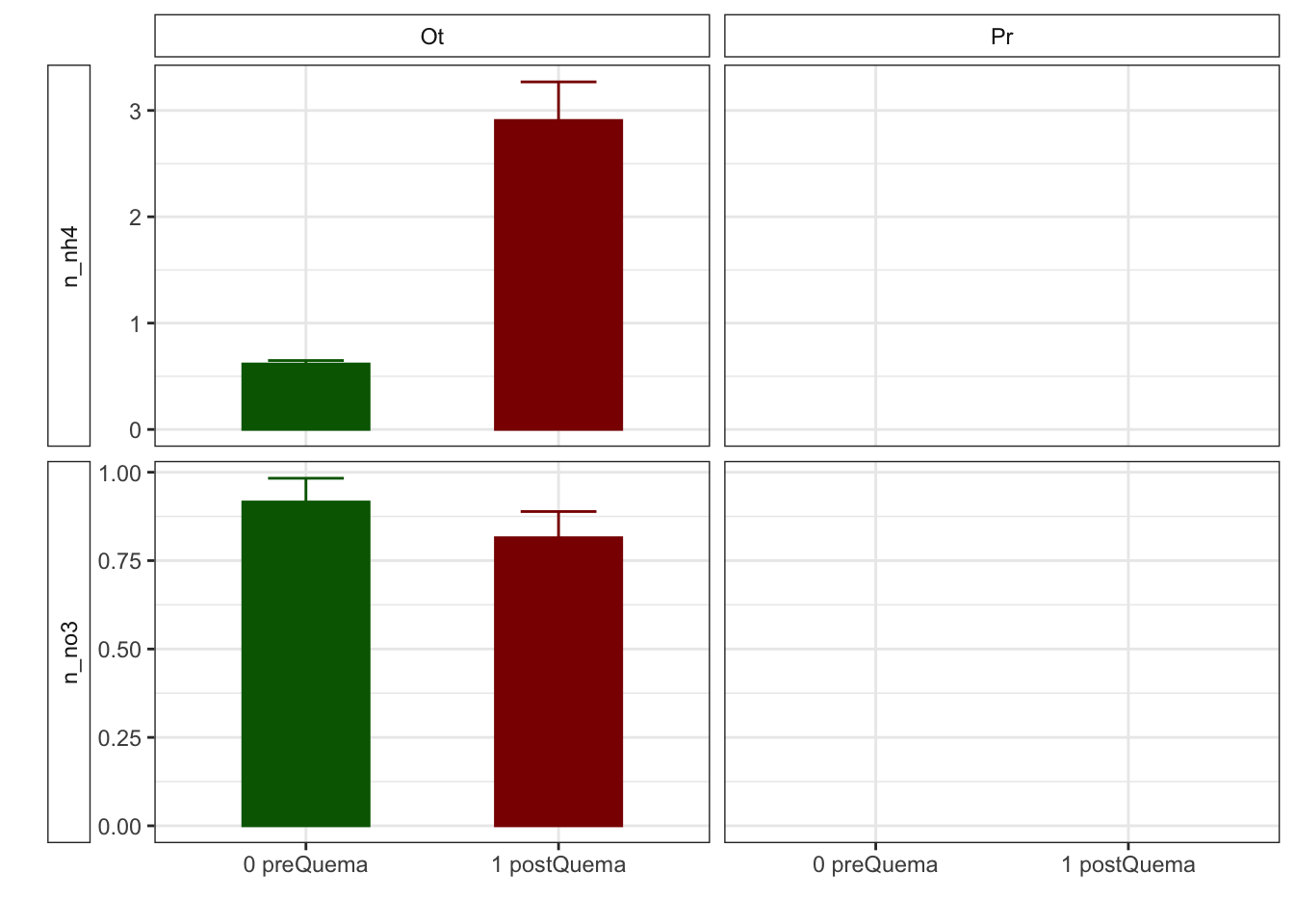
- We have only data for Autumn fire
- The approach will be the following: Apply non-parametric Wilcoxon test to compare pre and postFire
        fecha
estacion 0 preQuema 1 postQuema
      Ot         48          43
Model
NO3
Model
General Overview
Mean + SE table
| Characteristic | 0 preQuema | 1 postQuema | ||
|---|---|---|---|---|
| Ot, N = 481 | Pr, N = 241 | Ot, N = 481 | Pr, N = 241 | |
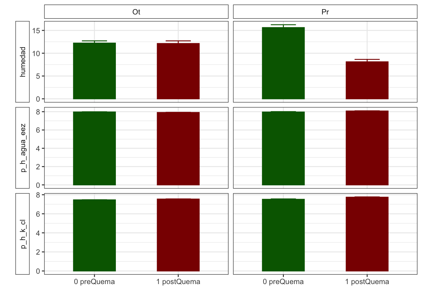
| humedad | 12.22 (0.50) | 15.62 (0.63) | 12.13 (0.59) | 8.11 (0.53) |
| n_nh4 | 0.62 (0.03) | NA (NA) | 2.91 (0.36) | NA (NA) |
| n_no3 | 0.92 (0.07) | NA (NA) | 0.81 (0.07) | NA (NA) |
| fe_percent | 1.86 (0.07) | 1.95 (0.08) | 1.80 (0.04) | 1.95 (0.09) |
| k_percent | 0.45 (0.03) | 0.79 (0.06) | 0.41 (0.03) | 0.75 (0.06) |
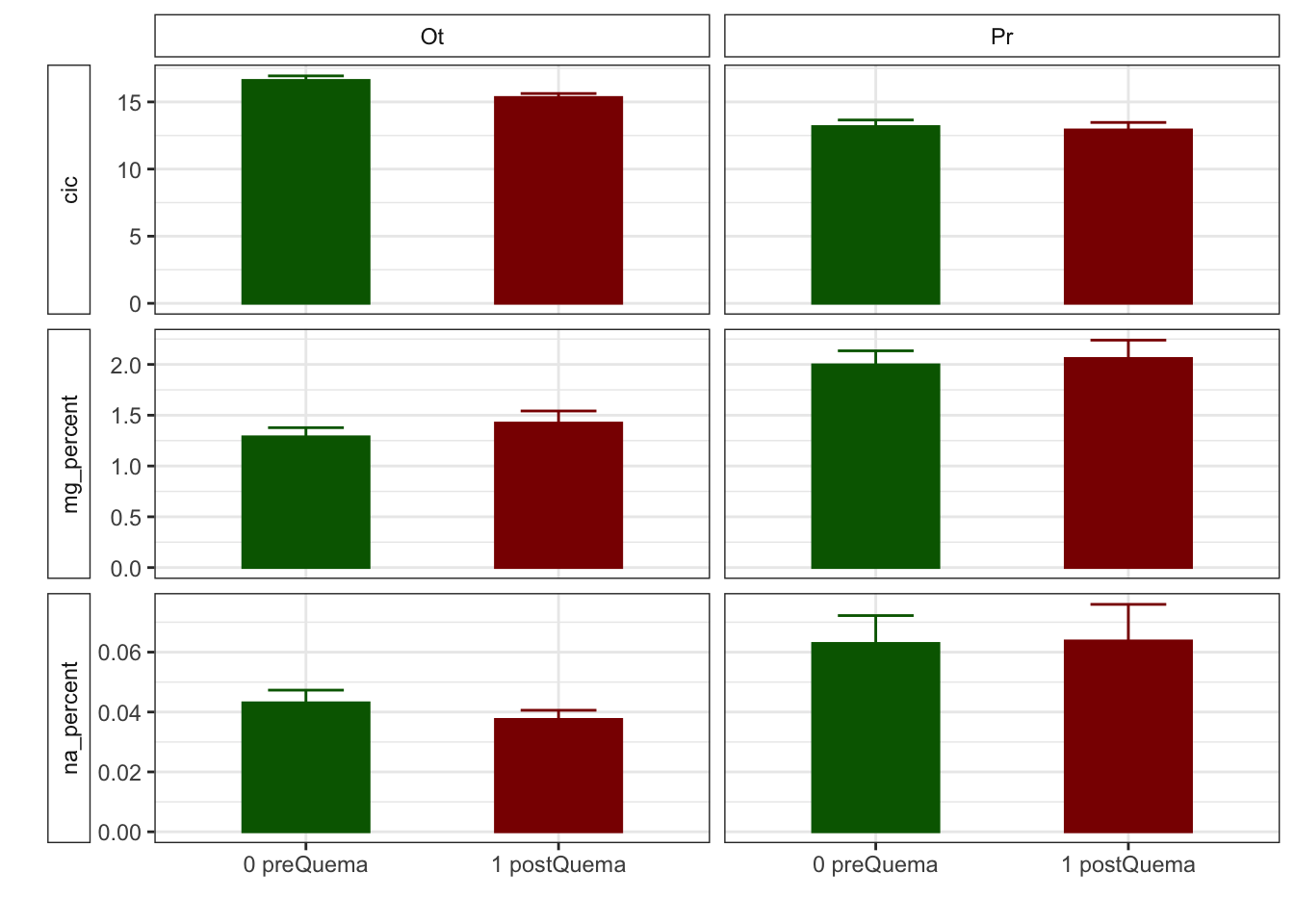
| mg_percent | 1.29 (0.09) | 2.00 (0.14) | 1.42 (0.12) | 2.06 (0.18) |
| na_percent | 0.04 (0.00) | 0.06 (0.01) | 0.04 (0.00) | 0.06 (0.01) |
| n_percent | 0.22 (0.01) | 0.19 (0.02) | 0.29 (0.02) | 0.18 (0.01) |
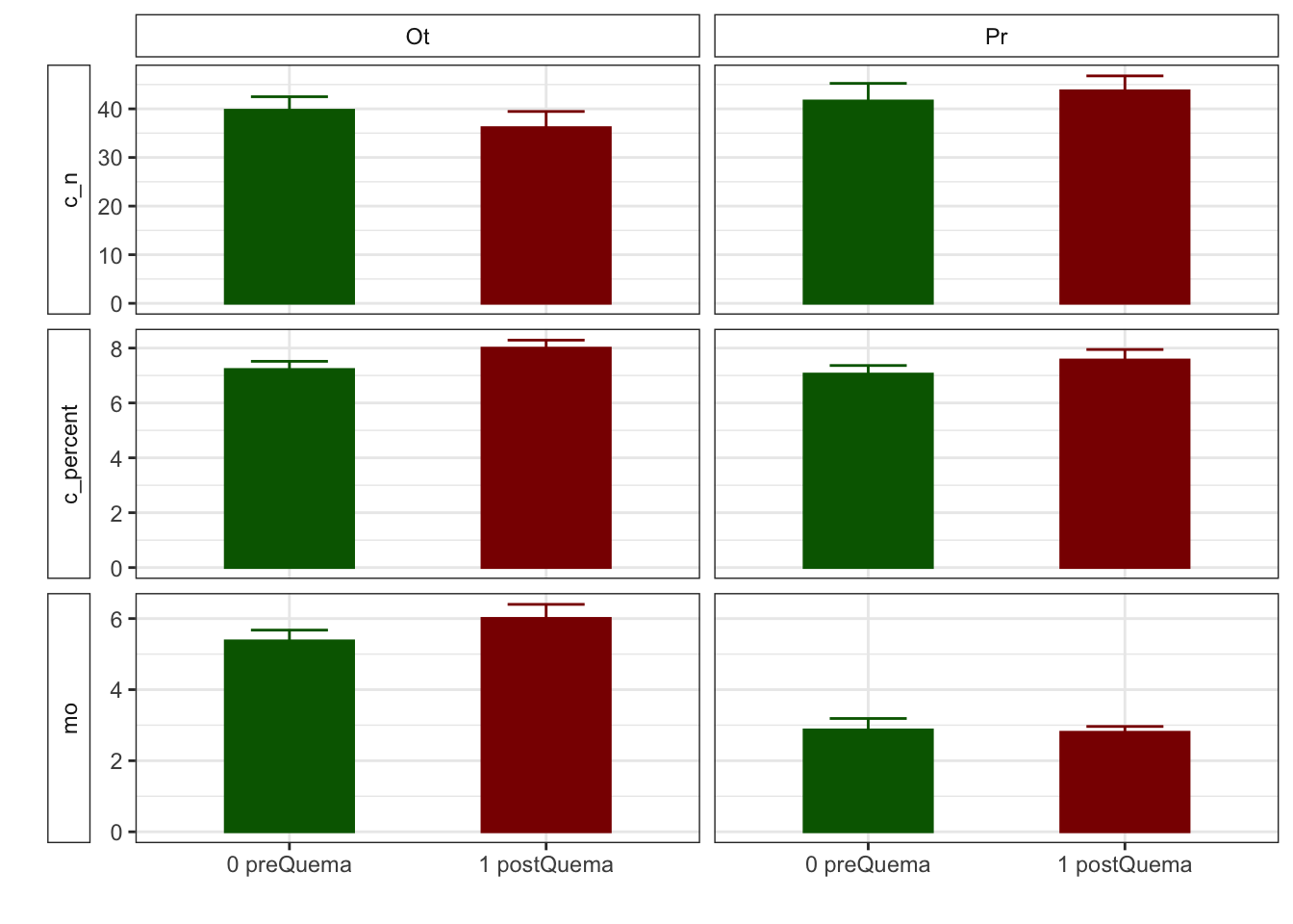
| c_percent | 7.22 (0.30) | 7.05 (0.31) | 8.00 (0.29) | 7.57 (0.38) |
| c_n | 39.72 (2.77) | 41.62 (3.62) | 36.14 (3.32) | 43.72 (3.06) |
| cic | 16.60 (0.34) | 13.17 (0.49) | 15.33 (0.29) | 12.92 (0.55) |
| p | 3.83 (0.17) | 6.75 (0.92) | 5.20 (0.24) | 5.88 (0.25) |
| mo | 5.37 (0.30) | 2.87 (0.32) | 6.00 (0.39) | 2.80 (0.16) |
| p_h_k_cl | 7.46 (0.02) | 7.52 (0.04) | 7.54 (0.02) | 7.74 (0.03) |
| p_h_agua_eez | 7.97 (0.02) | 7.97 (0.04) | 7.91 (0.02) | 8.07 (0.02) |
|
1
Mean (std.error)
|
||||
| Characteristic | Ot | Pr | ||
|---|---|---|---|---|
| 0 preQuema, N = 481 | 1 postQuema, N = 481 | 0 preQuema, N = 241 | 1 postQuema, N = 241 | |
| humedad | 12.22 (0.50) | 12.13 (0.59) | 15.62 (0.63) | 8.11 (0.53) |
| n_nh4 | 0.62 (0.03) | 2.91 (0.36) | NA (NA) | NA (NA) |
| n_no3 | 0.92 (0.07) | 0.81 (0.07) | NA (NA) | NA (NA) |
| fe_percent | 1.86 (0.07) | 1.80 (0.04) | 1.95 (0.08) | 1.95 (0.09) |
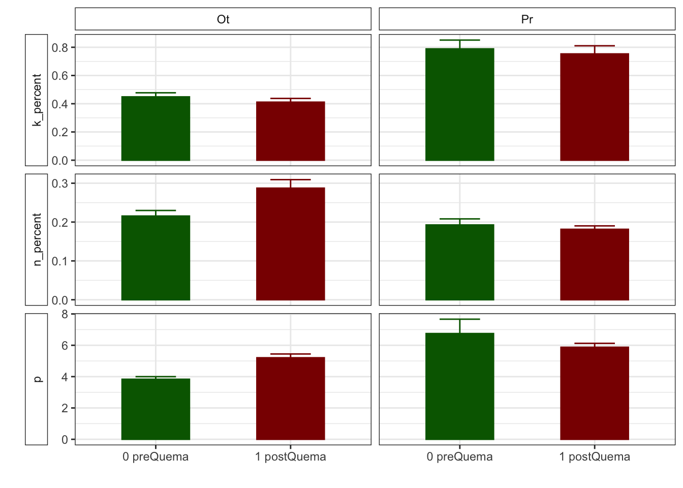
| k_percent | 0.45 (0.03) | 0.41 (0.03) | 0.79 (0.06) | 0.75 (0.06) |
| mg_percent | 1.29 (0.09) | 1.42 (0.12) | 2.00 (0.14) | 2.06 (0.18) |
| na_percent | 0.04 (0.00) | 0.04 (0.00) | 0.06 (0.01) | 0.06 (0.01) |
| n_percent | 0.22 (0.01) | 0.29 (0.02) | 0.19 (0.02) | 0.18 (0.01) |
| c_percent | 7.22 (0.30) | 8.00 (0.29) | 7.05 (0.31) | 7.57 (0.38) |
| c_n | 39.72 (2.77) | 36.14 (3.32) | 41.62 (3.62) | 43.72 (3.06) |
| cic | 16.60 (0.34) | 15.33 (0.29) | 13.17 (0.49) | 12.92 (0.55) |
| p | 3.83 (0.17) | 5.20 (0.24) | 6.75 (0.92) | 5.88 (0.25) |
| mo | 5.37 (0.30) | 6.00 (0.39) | 2.87 (0.32) | 2.80 (0.16) |
| p_h_k_cl | 7.46 (0.02) | 7.54 (0.02) | 7.52 (0.04) | 7.74 (0.03) |
| p_h_agua_eez | 7.97 (0.02) | 7.91 (0.02) | 7.97 (0.04) | 8.07 (0.02) |
|
1
Mean (std.error)
|
||||
Figures
| Version | Author | Date |
|---|---|---|
| 389b963 | ajpelu | 2021-09-14 |
| Version | Author | Date |
|---|---|---|
| 389b963 | ajpelu | 2021-09-14 |
| Version | Author | Date |
|---|---|---|
| 389b963 | ajpelu | 2021-09-14 |
Anovas table
| Variables | F | p | F | p | F | p |
|---|---|---|---|---|---|---|
| c_n | 0.560 | 0.471 | 0.055 | 0.815 | 0.803 | 0.372 |
| cic | 9.836 | 0.011 | 5.112 | 0.025 | 2.303 | 0.132 |
| k_percent | 8.325 | 0.016 | 1.919 | 0.168 | 0.001 | 0.976 |
| mg_percent | 4.011 | 0.073 | 0.959 | 0.329 | 0.130 | 0.719 |
| mo | 35.185 | 0.000 | 0.602 | 0.439 | 0.914 | 0.341 |
| n_nh4 | NA | NA | 403.000 | 0.000 | NA | NA |
| n_no3 | NA | NA | 1198.500 | 0.187 | NA | NA |
| p | 8.169 | 0.017 | 0.454 | 0.502 | 9.306 | 0.003 |
| p_h_agua_eez | 9.290 | 0.012 | 0.989 | 0.322 | 10.511 | 0.002 |
| p_h_k_cl | 5.701 | 0.038 | 45.363 | 0.000 | 9.393 | 0.003 |
| humedad | 0.058 | 0.815 | 50.420 | 0.000 | 48.041 | 0.000 |
| n_percent | 7.294 | 0.007 | 5.121 | 0.024 | 2.671 | 0.102 |
| c_percent | 0.118 | 0.738 | 6.180 | 0.014 | 0.261 | 0.610 |
| na_percent | 2.571 | 0.109 | 0.735 | 0.391 | 0.070 | 0.791 |
Gráficos feos feísimos
| Version | Author | Date |
|---|---|---|
| 389b963 | ajpelu | 2021-09-14 |
| Version | Author | Date |
|---|---|---|
| 389b963 | ajpelu | 2021-09-14 |
| Version | Author | Date |
|---|---|---|
| 389b963 | ajpelu | 2021-09-14 |
| Version | Author | Date |
|---|---|---|
| 389b963 | ajpelu | 2021-09-14 |
| Version | Author | Date |
|---|---|---|
| 389b963 | ajpelu | 2021-09-14 |
R version 4.0.2 (2020-06-22)
Platform: x86_64-apple-darwin17.0 (64-bit)
Running under: macOS Catalina 10.15.3

Matrix products: default
BLAS:   /Library/Frameworks/R.framework/Versions/4.0/Resources/lib/libRblas.dylib
LAPACK: /Library/Frameworks/R.framework/Versions/4.0/Resources/lib/libRlapack.dylib

locale:
[1] en_US.UTF-8/en_US.UTF-8/en_US.UTF-8/C/en_US.UTF-8/en_US.UTF-8

attached base packages:
[1] stats     graphics  grDevices utils     datasets  methods   base

other attached packages:
 [1] kableExtra_1.3.1   gtsummary_1.4.2    plotrix_3.8-1      glmmTMB_1.0.2.1
 [5] afex_0.28-1        performance_0.7.2  multcomp_1.4-16    TH.data_1.0-10
 [9] mvtnorm_1.1-1      emmeans_1.5.4      lmerTest_3.1-3     lme4_1.1-27.1
[13] Matrix_1.3-2       fitdistrplus_1.1-3 survival_3.2-7     MASS_7.3-53
[17] ggpubr_0.4.0       janitor_2.1.0      here_1.0.1         forcats_0.5.1
[21] stringr_1.4.0      dplyr_1.0.6        purrr_0.3.4        readr_1.4.0
[25] tidyr_1.1.3        tibble_3.1.2       ggplot2_3.3.5      tidyverse_1.3.1
[29] rmdformats_1.0.1   knitr_1.31         workflowr_1.6.2

loaded via a namespace (and not attached):
  [1] minqa_1.2.4         colorspace_2.0-0    ggsignif_0.6.0
  [4] ellipsis_0.3.2      rio_0.5.16          rprojroot_2.0.2
  [7] estimability_1.3    snakecase_0.11.0    fs_1.5.0
 [10] rstudioapi_0.13     farver_2.0.3        fansi_0.4.2
 [13] lubridate_1.7.10    xml2_1.3.2          codetools_0.2-18
 [16] splines_4.0.2       jsonlite_1.7.2      nloptr_1.2.2.2
 [19] gt_0.3.0            pbkrtest_0.5-0.1    broom_0.7.9
 [22] dbplyr_2.1.1        compiler_4.0.2      httr_1.4.2
 [25] backports_1.2.1     assertthat_0.2.1    fastmap_1.1.0
 [28] cli_2.5.0           formatR_1.8         later_1.1.0.1
 [31] htmltools_0.5.2     tools_4.0.2         coda_0.19-4
 [34] gtable_0.3.0        glue_1.4.2          reshape2_1.4.4
 [37] Rcpp_1.0.7          carData_3.0-4       cellranger_1.1.0
 [40] jquerylib_0.1.3     vctrs_0.3.8         nlme_3.1-152
 [43] broom.helpers_1.3.0 insight_0.14.4      xfun_0.23
 [46] openxlsx_4.2.3      rvest_1.0.0         lifecycle_1.0.0
 [49] rstatix_0.6.0       zoo_1.8-8           scales_1.1.1
 [52] hms_1.0.0           promises_1.2.0.1    parallel_4.0.2
 [55] sandwich_3.0-0      TMB_1.7.19          yaml_2.2.1
 [58] curl_4.3            sass_0.3.1          stringi_1.7.4
 [61] highr_0.8           checkmate_2.0.0     boot_1.3-26
 [64] zip_2.1.1           commonmark_1.7      rlang_0.4.10
 [67] pkgconfig_2.0.3     evaluate_0.14       lattice_0.20-41
 [70] labeling_0.4.2      tidyselect_1.1.1    plyr_1.8.6
 [73] magrittr_2.0.1      bookdown_0.21.6     R6_2.5.0
 [76] generics_0.1.0      DBI_1.1.1           pillar_1.6.1
 [79] haven_2.3.1         whisker_0.4         foreign_0.8-81
 [82] withr_2.4.1         abind_1.4-5         modelr_0.1.8
 [85] crayon_1.4.1        car_3.0-10          utf8_1.1.4
 [88] rmarkdown_2.8       grid_4.0.2          readxl_1.3.1
 [91] data.table_1.14.0   git2r_0.28.0        webshot_0.5.2
 [94] reprex_2.0.0        digest_0.6.27       xtable_1.8-4
 [97] httpuv_1.5.5        numDeriv_2016.8-1.1 munsell_0.5.0
[100] viridisLite_0.3.0   bslib_0.2.4