Last updated: 2021-09-07

Checks: 6 1

Knit directory: soil_alcontar/

This reproducible R Markdown analysis was created with workflowr (version 1.6.2). The Checks tab describes the reproducibility checks that were applied when the results were created. The Past versions tab lists the development history.

R Markdown file: up-to-date

Great! Since the R Markdown file has been committed to the Git repository, you know the exact version of the code that produced these results.

Environment: empty

Great job! The global environment was empty. Objects defined in the global environment can affect the analysis in your R Markdown file in unknown ways. For reproduciblity it’s best to always run the code in an empty environment.

Seed: set.seed(20210907)

The command set.seed(20210907) was run prior to running the code in the R Markdown file. Setting a seed ensures that any results that rely on randomness, e.g. subsampling or permutations, are reproducible.

Session information: recorded

Great job! Recording the operating system, R version, and package versions is critical for reproducibility.

Cache: detected

The following chunks had caches available:

pkgs
prepare-data
session-info-chunk-inserted-by-workflowr
unnamed-chunk-1
unnamed-chunk-10
unnamed-chunk-11
unnamed-chunk-12
unnamed-chunk-13
unnamed-chunk-14
unnamed-chunk-15
unnamed-chunk-16
unnamed-chunk-17
unnamed-chunk-18
unnamed-chunk-19
unnamed-chunk-2
unnamed-chunk-20
unnamed-chunk-21
unnamed-chunk-22
unnamed-chunk-23
unnamed-chunk-24
unnamed-chunk-25
unnamed-chunk-26
unnamed-chunk-27
unnamed-chunk-28
unnamed-chunk-29
unnamed-chunk-3
unnamed-chunk-30
unnamed-chunk-31
unnamed-chunk-32
unnamed-chunk-33
unnamed-chunk-34
unnamed-chunk-35
unnamed-chunk-36
unnamed-chunk-37
unnamed-chunk-38
unnamed-chunk-39
unnamed-chunk-4
unnamed-chunk-40
unnamed-chunk-41
unnamed-chunk-42
unnamed-chunk-43
unnamed-chunk-44
unnamed-chunk-45
unnamed-chunk-46
unnamed-chunk-47
unnamed-chunk-48
unnamed-chunk-49
unnamed-chunk-5
unnamed-chunk-50
unnamed-chunk-51
unnamed-chunk-52
unnamed-chunk-53
unnamed-chunk-54
unnamed-chunk-55
unnamed-chunk-56
unnamed-chunk-57
unnamed-chunk-58
unnamed-chunk-59
unnamed-chunk-6
unnamed-chunk-60
unnamed-chunk-61
unnamed-chunk-62
unnamed-chunk-63
unnamed-chunk-64
unnamed-chunk-65
unnamed-chunk-66
unnamed-chunk-67
unnamed-chunk-68
unnamed-chunk-69
unnamed-chunk-7
unnamed-chunk-70
unnamed-chunk-71
unnamed-chunk-72
unnamed-chunk-73
unnamed-chunk-74
unnamed-chunk-75
unnamed-chunk-76
unnamed-chunk-8
unnamed-chunk-9

To ensure reproducibility of the results, delete the cache directory analysis_pre_post_cache and re-run the analysis. To have workflowr automatically delete the cache directory prior to building the file, set delete_cache = TRUE when running wflow_build() or wflow_publish().

File paths: relative

Great job! Using relative paths to the files within your workflowr project makes it easier to run your code on other machines.

Repository version: 2c59a9d

Great! You are using Git for version control. Tracking code development and connecting the code version to the results is critical for reproducibility.

The results in this page were generated with repository version 2c59a9d. See the Past versions tab to see a history of the changes made to the R Markdown and HTML files.

Note that you need to be careful to ensure that all relevant files for the analysis have been committed to Git prior to generating the results (you can use wflow_publish or wflow_git_commit). workflowr only checks the R Markdown file, but you know if there are other scripts or data files that it depends on. Below is the status of the Git repository when the results were generated:


Ignored files:
    Ignored:    .RData
    Ignored:    .Rhistory
    Ignored:    .Rproj.user/C369E4F4/
    Ignored:    .Rproj.user/shared/notebooks/3F603CAC-map/
    Ignored:    .Rproj.user/shared/notebooks/4E13660A-temporal_comparison/
    Ignored:    .Rproj.user/shared/notebooks/7ADB7089-Untitled/
    Ignored:    .Rproj.user/shared/notebooks/827D0727-analysis_pre_post/
    Ignored:    .Rproj.user/shared/notebooks/8A21BEE6-analysis_pre_post/
    Ignored:    .Rproj.user/shared/notebooks/A3F813C2-index/
    Ignored:    .Rproj.user/shared/notebooks/F2779D03-index/

Untracked files:
    Untracked:  analysis/analysis_pre_post_cache/
    Untracked:  analysis/test.Rmd
    Untracked:  data/spatial/lucdeme/
    Untracked:  map.Rmd

Unstaged changes:
    Modified:   data/Resultados_Suelos_2018_2021_v2.xlsx
    Modified:   data/spatial/.DS_Store
    Deleted:    index.Rmd
    Modified:   scripts/00_prepare_data.R
    Modified:   temporal_comparison.Rmd

Note that any generated files, e.g. HTML, png, CSS, etc., are not included in this status report because it is ok for generated content to have uncommitted changes.

These are the previous versions of the repository in which changes were made to the R Markdown (analysis/analysis_pre_post.Rmd) and HTML (docs/analysis_pre_post.html) files. If you’ve configured a remote Git repository (see ?wflow_git_remote), click on the hyperlinks in the table below to view the files as they were in that past version.

File	Version	Author	Date	Message
Rmd	2c59a9d	ajpelu	2021-09-07	update
html	68358ce	ajpelu	2021-09-07	Build site.
Rmd	6ef970d	ajpelu	2021-09-07	add plot
html	bfa8071	ajpelu	2021-09-07	Build site.
Rmd	dc87911	ajpelu	2021-09-07	include pre post analysis

Prepare data

raw_soil <- readxl::read_excel(here::here("data/Resultados_Suelos_2018_2021_v2.xlsx"), 
    sheet = "SEGUIMIENTO_MUESTRAS_SUELOS") %>% janitor::clean_names() %>% mutate(treatment_name = case_when(str_detect(geo_parcela_nombre, 
    "NP_") ~ "Autumn Burning / No Browsing", str_detect(geo_parcela_nombre, "PR_") ~ 
    "Spring Burning / Browsing", str_detect(geo_parcela_nombre, "P_") ~ "Autumn Burning / Browsing"), 
    zona = case_when(str_detect(geo_parcela_nombre, "NP_") ~ "NP", str_detect(geo_parcela_nombre, 
        "PR_") ~ "PR", str_detect(geo_parcela_nombre, "P_") ~ "P"), fecha = lubridate::ymd(fecha), 
    pre_post_quema = case_when(pre_post_quema == "Prequema" ~ "0 Pre", pre_post_quema == 
        "Postquema" ~ "1 Post"))

Select data pre- and intermediately post-fire (first post-fire sampling: “2018-12-20” and “2019-05-09” for autumn and spring fires respectively)

soil <- raw_soil %>% filter(fecha %in% lubridate::ymd(c("2018-12-11", "2018-12-20", 
    "2019-04-24", "2019-05-09"))) %>% mutate(zona = as.factor(zona), pre_post_quema = as.factor(pre_post_quema))

Structure of the data

              zona
pre_post_quema NP  P PR
        0 Pre  24 24 24
        1 Post 24 24 24

Modellize

For each response variable, the approach modelling is

\(Y \sim zona (P|NP|PR) + Fecha(pre|post) + zona \times Fecha\)

using the “(1|zona:geo_parcela_nombre)” as nested random effects
Then explore error distribution of the variable response and model diagnostics
Select the appropiate error distribution and use LMM or GLMM
Explore Post-hoc
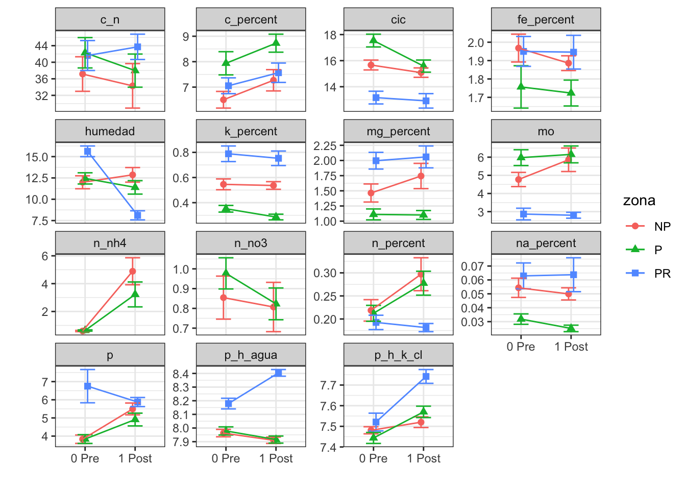
Plot interactions

Humedad

Check distribution

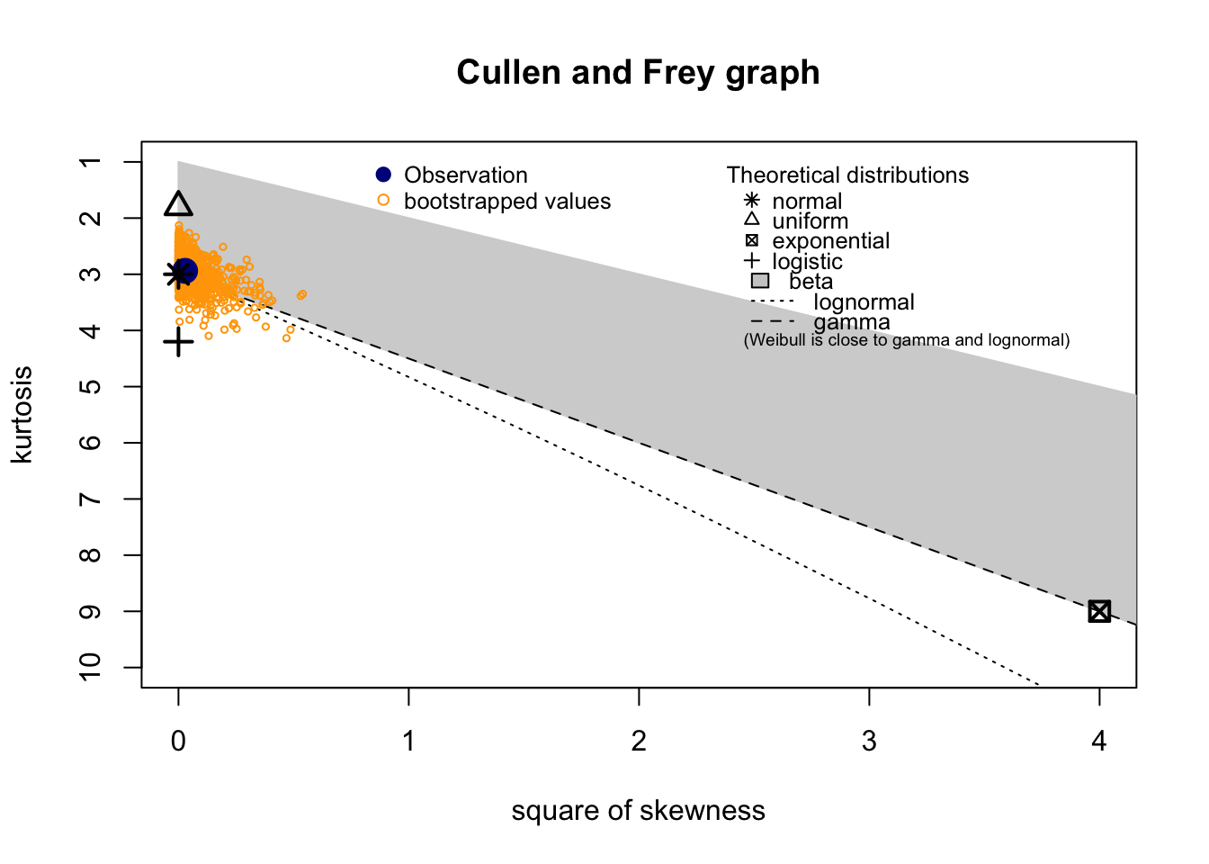
summary statistics
------
min:  2.961538   max:  23.90476 
median:  11.90231 
mean:  12.0709 
estimated sd:  4.08543 
estimated skewness:  0.1696677 
estimated kurtosis:  2.93929

Normality & Homocedasticity

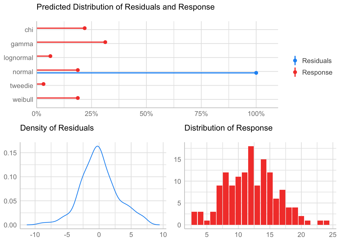
[1] "Variances homogeneity?"

OK: Variances in each of the groups are the same (Bartlett Test, p = 0.257).

[1] "Normality?"

OK: residuals appear as normally distributed (p = 0.096).

[1] "Normality, Random effects"

Group: zona:geo_parcela_nombre
(Intercept) OK: random effects appear as normally distributed (p = 0.958).

Model

Type III Analysis of Variance Table with Satterthwaite's method
                    Sum Sq Mean Sq NumDF DenDF F value    Pr(>F)    
pre_post_quema      236.42 236.416     1   129 26.1050 1.136e-06 ***
zona                  1.46   0.728     2     9  0.0803    0.9235    
pre_post_quema:zona 462.22 231.109     2   129 25.5190 4.593e-10 ***
---
Signif. codes:  0 '***' 0.001 '**' 0.01 '*' 0.05 '.' 0.1 ' ' 1

Post-hoc

$`emmeans of pre_post_quema`
 pre_post_quema emmean    SE   df lower.CL upper.CL
 0 Pre            13.4 0.676 12.1    11.88     14.8
 1 Post           10.8 0.676 12.1     9.32     12.3

Results are averaged over the levels of: zona 
Degrees-of-freedom method: kenward-roger 
Confidence level used: 0.95 

$`pairwise differences of pre_post_quema`
 1              estimate    SE  df t.ratio p.value
 0 Pre - 1 Post     2.56 0.502 129 5.109   <.0001 

Results are averaged over the levels of: zona 
Degrees-of-freedom method: kenward-roger

$`emmeans of zona`
 zona emmean   SE df lower.CL upper.CL
 NP     12.4 1.09  9     9.97     14.9
 P      11.9 1.09  9     9.46     14.4
 PR     11.9 1.09  9     9.41     14.3

Results are averaged over the levels of: pre_post_quema 
Degrees-of-freedom method: kenward-roger 
Confidence level used: 0.95 

$`pairwise differences of zona`
 1       estimate   SE df t.ratio p.value
 NP - P    0.5060 1.54  9 0.329   0.9424 
 NP - PR   0.5579 1.54  9 0.363   0.9306 
 P - PR    0.0518 1.54  9 0.034   0.9994 

Results are averaged over the levels of: pre_post_quema 
Degrees-of-freedom method: kenward-roger 
P value adjustment: tukey method for comparing a family of 3 estimates

$`emmeans of pre_post_quema | zona`
zona = NP:
 pre_post_quema emmean   SE   df lower.CL upper.CL
 0 Pre           11.99 1.17 12.1     9.44     14.5
 1 Post          12.86 1.17 12.1    10.31     15.4

zona = P:
 pre_post_quema emmean   SE   df lower.CL upper.CL
 0 Pre           12.45 1.17 12.1     9.90     15.0
 1 Post          11.39 1.17 12.1     8.84     13.9

zona = PR:
 pre_post_quema emmean   SE   df lower.CL upper.CL
 0 Pre           15.62 1.17 12.1    13.07     18.2
 1 Post           8.11 1.17 12.1     5.57     10.7

Degrees-of-freedom method: kenward-roger 
Confidence level used: 0.95 

$`pairwise differences of pre_post_quema | zona`
zona = NP:
 2              estimate    SE  df t.ratio p.value
 0 Pre - 1 Post   -0.872 0.869 129 -1.004  0.3171 

zona = P:
 2              estimate    SE  df t.ratio p.value
 0 Pre - 1 Post    1.054 0.869 129  1.213  0.2273 

zona = PR:
 2              estimate    SE  df t.ratio p.value
 0 Pre - 1 Post    7.507 0.869 129  8.641  <.0001 

Degrees-of-freedom method: kenward-roger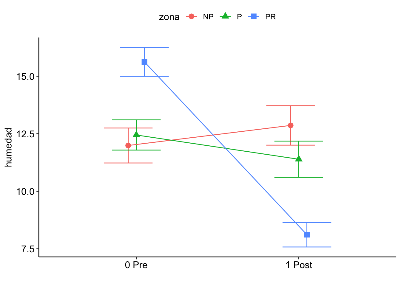

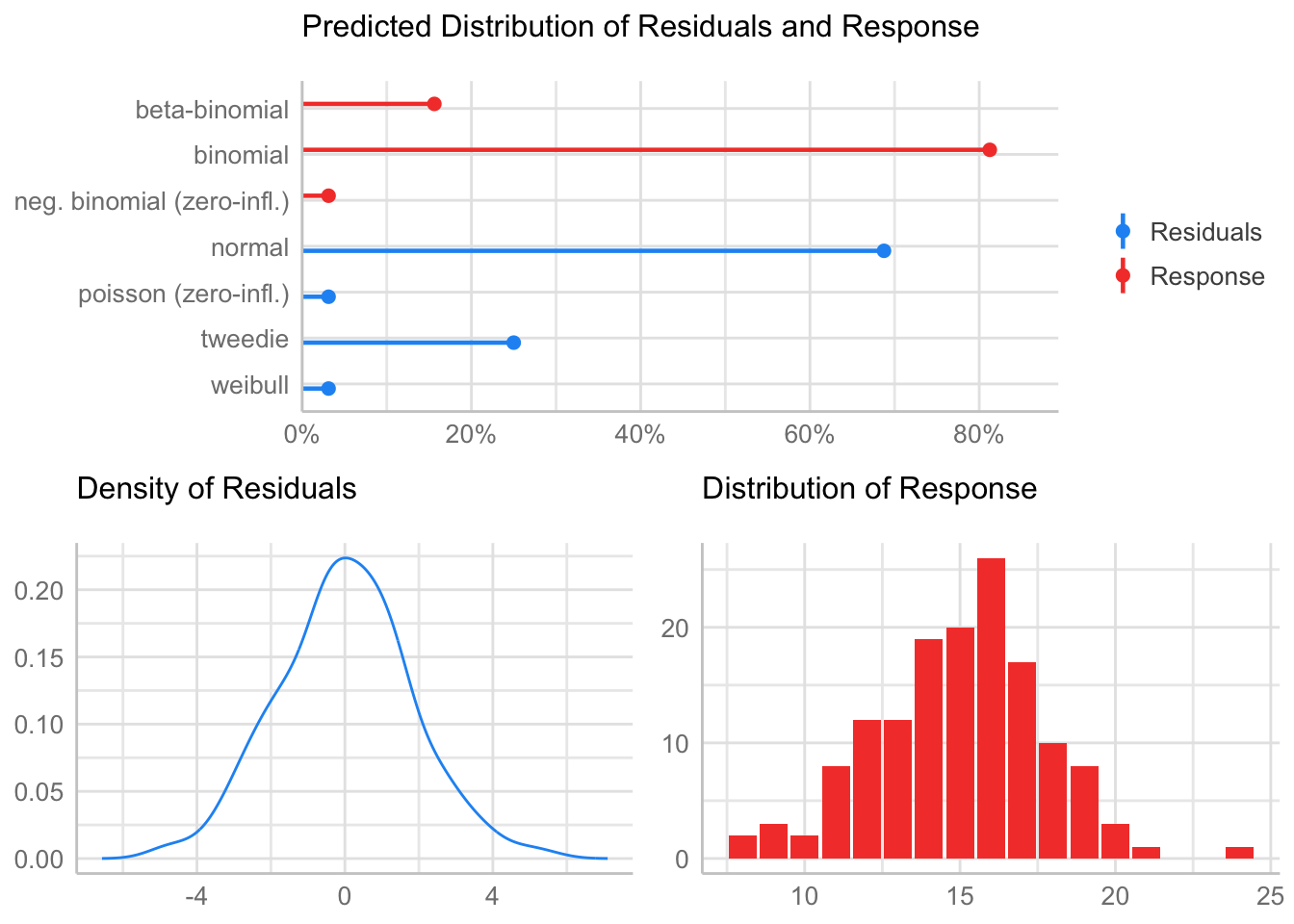
CIC

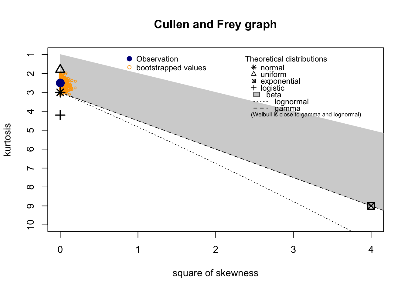
Check distribution

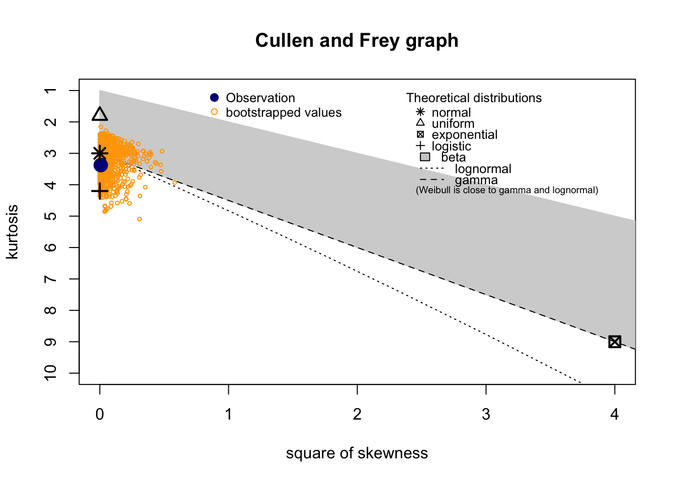
summary statistics
------
min:  8   max:  24 
median:  15 
mean:  14.99306 
estimated sd:  2.726448 
estimated skewness:  -0.08707462 
estimated kurtosis:  3.374256

Normality & Homocedasticity

[1] "Variances homogeneity?"

OK: Variances in each of the groups are the same (Bartlett Test, p = 0.313).

[1] "Normality?"

OK: residuals appear as normally distributed (p = 0.745).

[1] "Normality, Random effects"

Group: zona:geo_parcela_nombre
(Intercept) OK: random effects appear as normally distributed (p = 0.397).

Model

Type III Analysis of Variance Table with Satterthwaite's method
                    Sum Sq Mean Sq NumDF DenDF F value   Pr(>F)   
pre_post_quema      31.174 31.1736     1   129  8.7568 0.003671 **
zona                40.297 20.1484     2     9  5.6598 0.025614 * 
pre_post_quema:zona 19.681  9.8403     2   129  2.7642 0.066764 . 
---
Signif. codes:  0 '***' 0.001 '**' 0.01 '*' 0.05 '.' 0.1 ' ' 1

Post-hoc

$`emmeans of pre_post_quema`
 pre_post_quema emmean    SE   df lower.CL upper.CL
 0 Pre            15.5 0.462 11.5     14.4     16.5
 1 Post           14.5 0.462 11.5     13.5     15.5

Results are averaged over the levels of: zona 
Degrees-of-freedom method: kenward-roger 
Confidence level used: 0.95 

$`pairwise differences of pre_post_quema`
 1              estimate    SE  df t.ratio p.value
 0 Pre - 1 Post    0.931 0.314 129 2.959   0.0037 

Results are averaged over the levels of: zona 
Degrees-of-freedom method: kenward-roger

$`emmeans of zona`
 zona emmean    SE df lower.CL upper.CL
 NP     15.4 0.753  9     13.7     17.1
 P      16.6 0.753  9     14.9     18.3
 PR     13.0 0.753  9     11.3     14.7

Results are averaged over the levels of: pre_post_quema 
Degrees-of-freedom method: kenward-roger 
Confidence level used: 0.95 

$`pairwise differences of zona`
 1       estimate   SE df t.ratio p.value
 NP - P     -1.19 1.06  9 -1.115  0.5291 
 NP - PR     2.33 1.06  9  2.191  0.1262 
 P - PR      3.52 1.06  9  3.307  0.0225 

Results are averaged over the levels of: pre_post_quema 
Degrees-of-freedom method: kenward-roger 
P value adjustment: tukey method for comparing a family of 3 estimates

$`emmeans of pre_post_quema | zona`
zona = NP:
 pre_post_quema emmean    SE   df lower.CL upper.CL
 0 Pre            15.7 0.801 11.5     13.9     17.4
 1 Post           15.1 0.801 11.5     13.3     16.8

zona = P:
 pre_post_quema emmean    SE   df lower.CL upper.CL
 0 Pre            17.5 0.801 11.5     15.8     19.3
 1 Post           15.6 0.801 11.5     13.8     17.3

zona = PR:
 pre_post_quema emmean    SE   df lower.CL upper.CL
 0 Pre            13.2 0.801 11.5     11.4     14.9
 1 Post           12.9 0.801 11.5     11.2     14.7

Degrees-of-freedom method: kenward-roger 
Confidence level used: 0.95 

$`pairwise differences of pre_post_quema | zona`
zona = NP:
 2              estimate    SE  df t.ratio p.value
 0 Pre - 1 Post    0.583 0.545 129 1.071   0.2862 

zona = P:
 2              estimate    SE  df t.ratio p.value
 0 Pre - 1 Post    1.958 0.545 129 3.595   0.0005 

zona = PR:
 2              estimate    SE  df t.ratio p.value
 0 Pre - 1 Post    0.250 0.545 129 0.459   0.6470 

Degrees-of-freedom method: kenward-roger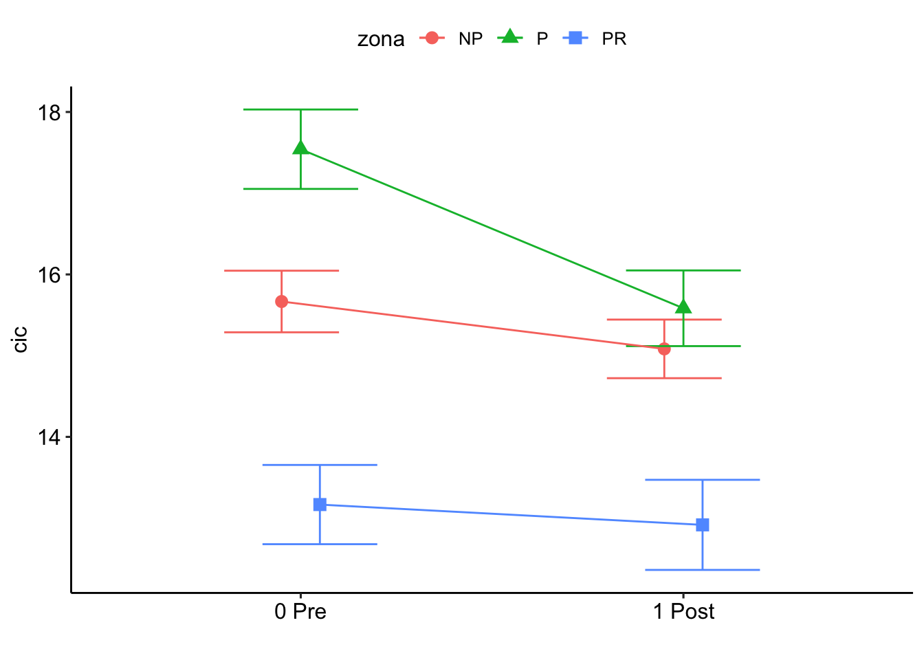

% C

Check distribution

summary statistics
------
min:  3.35   max:  12.5 
median:  7.57 
mean:  7.509167 
estimated sd:  1.9505 
estimated skewness:  0.03328586 
estimated kurtosis:  2.503996

Normality & Homocedasticity

[1] "Variances homogeneity?"

OK: Variances in each of the groups are the same (Bartlett Test, p = 0.434).

[1] "Normality?"

OK: residuals appear as normally distributed (p = 0.373).

[1] "Normality, Random effects"

Group: zona:geo_parcela_nombre
(Intercept) OK: random effects appear as normally distributed (p = 0.623).

Model

Type III Analysis of Variance Table with Satterthwaite's method
                     Sum Sq Mean Sq NumDF DenDF F value   Pr(>F)   
pre_post_quema      17.1120 17.1120     1   129  7.8770 0.005784 **
zona                 5.3708  2.6854     2     9  1.2361 0.335481   
pre_post_quema:zona  0.5673  0.2837     2   129  0.1306 0.877707   
---
Signif. codes:  0 '***' 0.001 '**' 0.01 '*' 0.05 '.' 0.1 ' ' 1

Post-hoc

$`emmeans of pre_post_quema`
 pre_post_quema emmean    SE   df lower.CL upper.CL
 0 Pre            7.16 0.405 10.9     6.27     8.06
 1 Post           7.85 0.405 10.9     6.96     8.75

Results are averaged over the levels of: zona 
Degrees-of-freedom method: kenward-roger 
Confidence level used: 0.95 

$`pairwise differences of pre_post_quema`
 1              estimate    SE  df t.ratio p.value
 0 Pre - 1 Post   -0.689 0.246 129 -2.807  0.0058 

Results are averaged over the levels of: zona 
Degrees-of-freedom method: kenward-roger

$`emmeans of zona`
 zona emmean    SE df lower.CL upper.CL
 NP     6.89 0.669  9     5.37     8.40
 P      8.33 0.669  9     6.82     9.84
 PR     7.31 0.669  9     5.80     8.82

Results are averaged over the levels of: pre_post_quema 
Degrees-of-freedom method: kenward-roger 
Confidence level used: 0.95 

$`pairwise differences of zona`
 1       estimate    SE df t.ratio p.value
 NP - P    -1.446 0.945  9 -1.529  0.3233 
 NP - PR   -0.424 0.945  9 -0.448  0.8965 
 P - PR     1.022 0.945  9  1.081  0.5483 

Results are averaged over the levels of: pre_post_quema 
Degrees-of-freedom method: kenward-roger 
P value adjustment: tukey method for comparing a family of 3 estimates

$`emmeans of pre_post_quema | zona`
zona = NP:
 pre_post_quema emmean    SE   df lower.CL upper.CL
 0 Pre            6.50 0.702 10.9     4.96     8.05
 1 Post           7.27 0.702 10.9     5.72     8.81

zona = P:
 pre_post_quema emmean    SE   df lower.CL upper.CL
 0 Pre            7.94 0.702 10.9     6.39     9.48
 1 Post           8.73 0.702 10.9     7.18    10.27

zona = PR:
 pre_post_quema emmean    SE   df lower.CL upper.CL
 0 Pre            7.05 0.702 10.9     5.51     8.60
 1 Post           7.57 0.702 10.9     6.02     9.11

Degrees-of-freedom method: kenward-roger 
Confidence level used: 0.95 

$`pairwise differences of pre_post_quema | zona`
zona = NP:
 2              estimate    SE  df t.ratio p.value
 0 Pre - 1 Post   -0.765 0.425 129 -1.799  0.0744 

zona = P:
 2              estimate    SE  df t.ratio p.value
 0 Pre - 1 Post   -0.790 0.425 129 -1.858  0.0655 

zona = PR:
 2              estimate    SE  df t.ratio p.value
 0 Pre - 1 Post   -0.512 0.425 129 -1.205  0.2306 

Degrees-of-freedom method: kenward-roger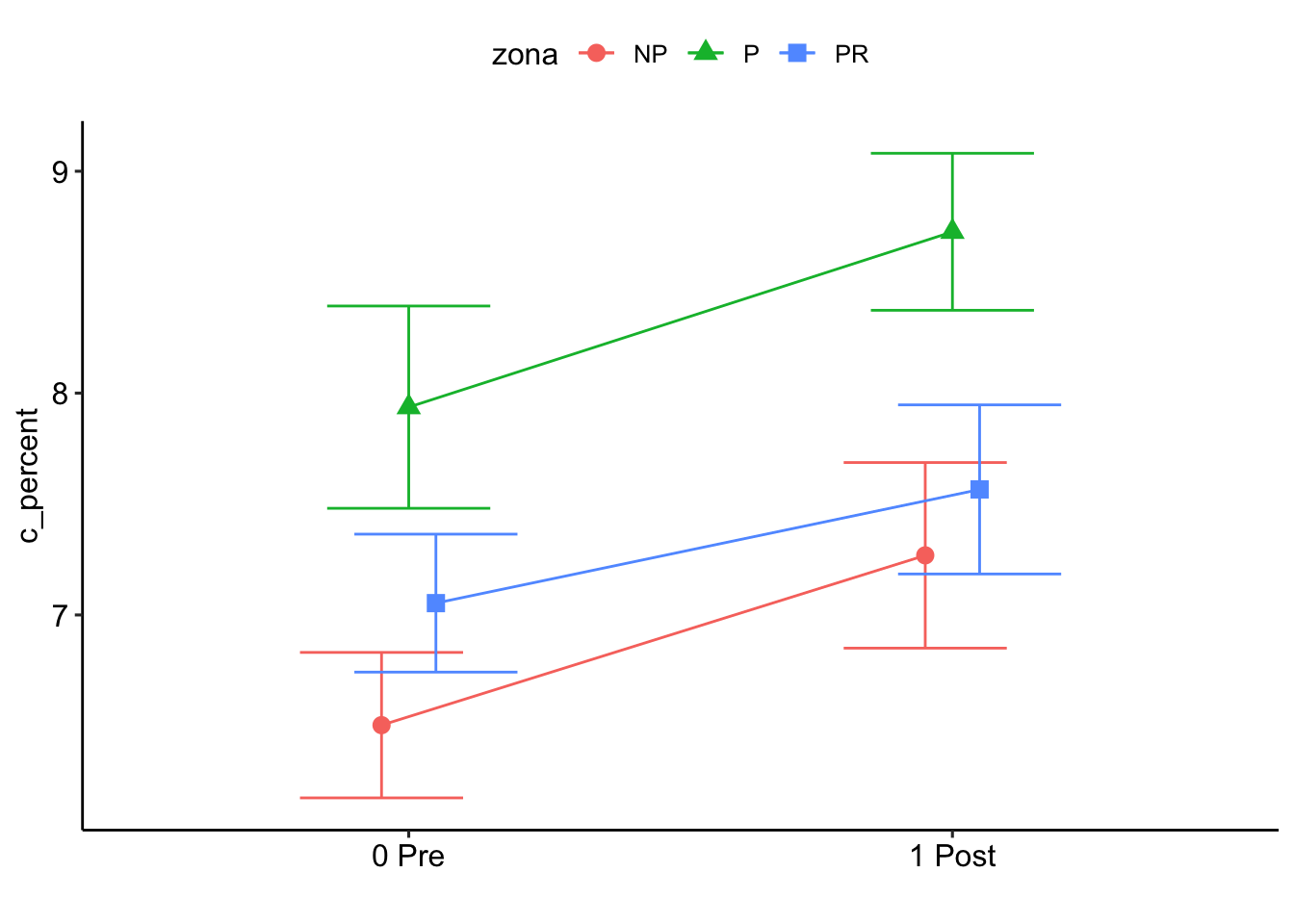

% Fe

Check distribution

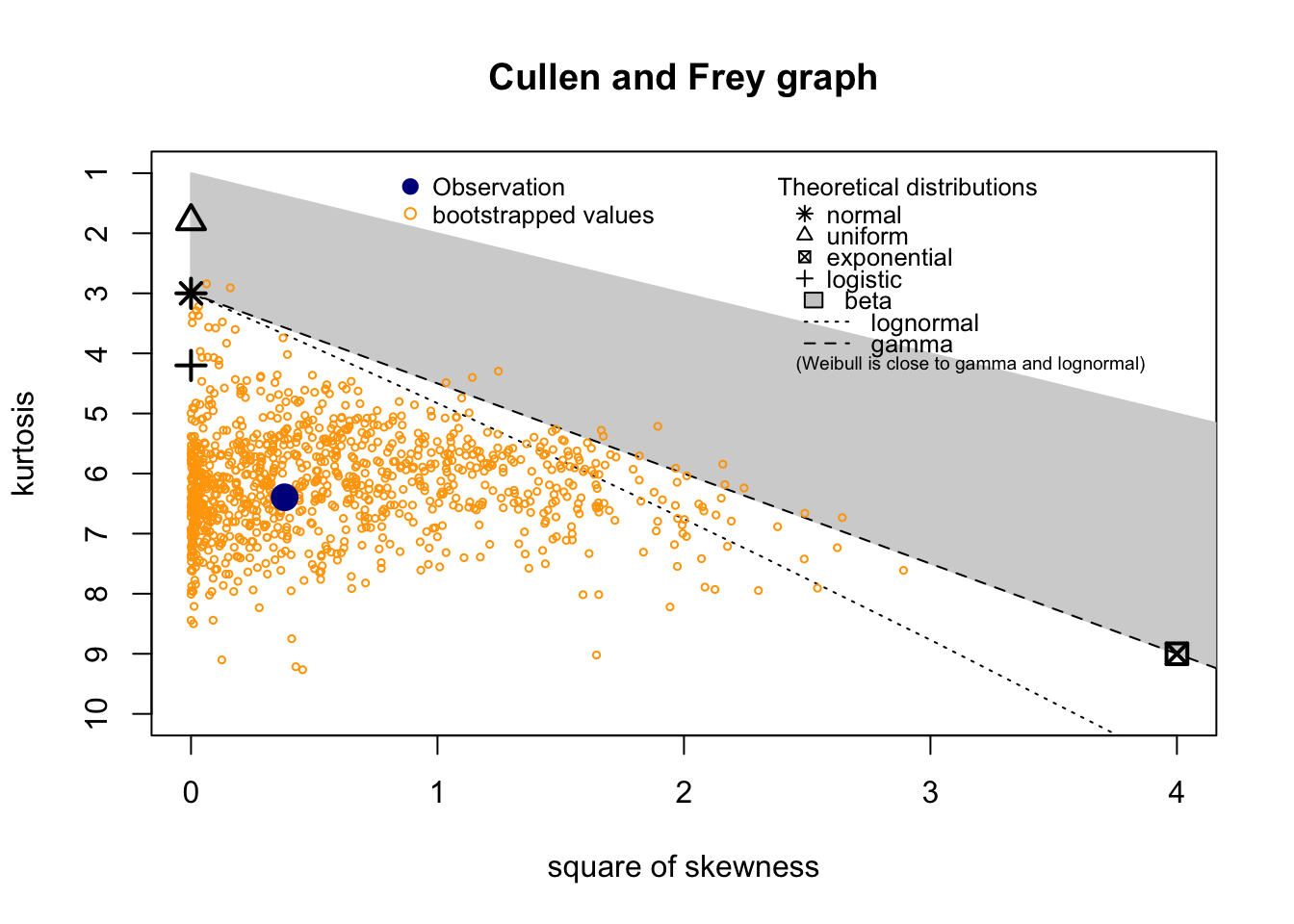
summary statistics
------
min:  0.341   max:  3.35 
median:  1.858 
mean:  1.87166 
estimated sd:  0.4077216 
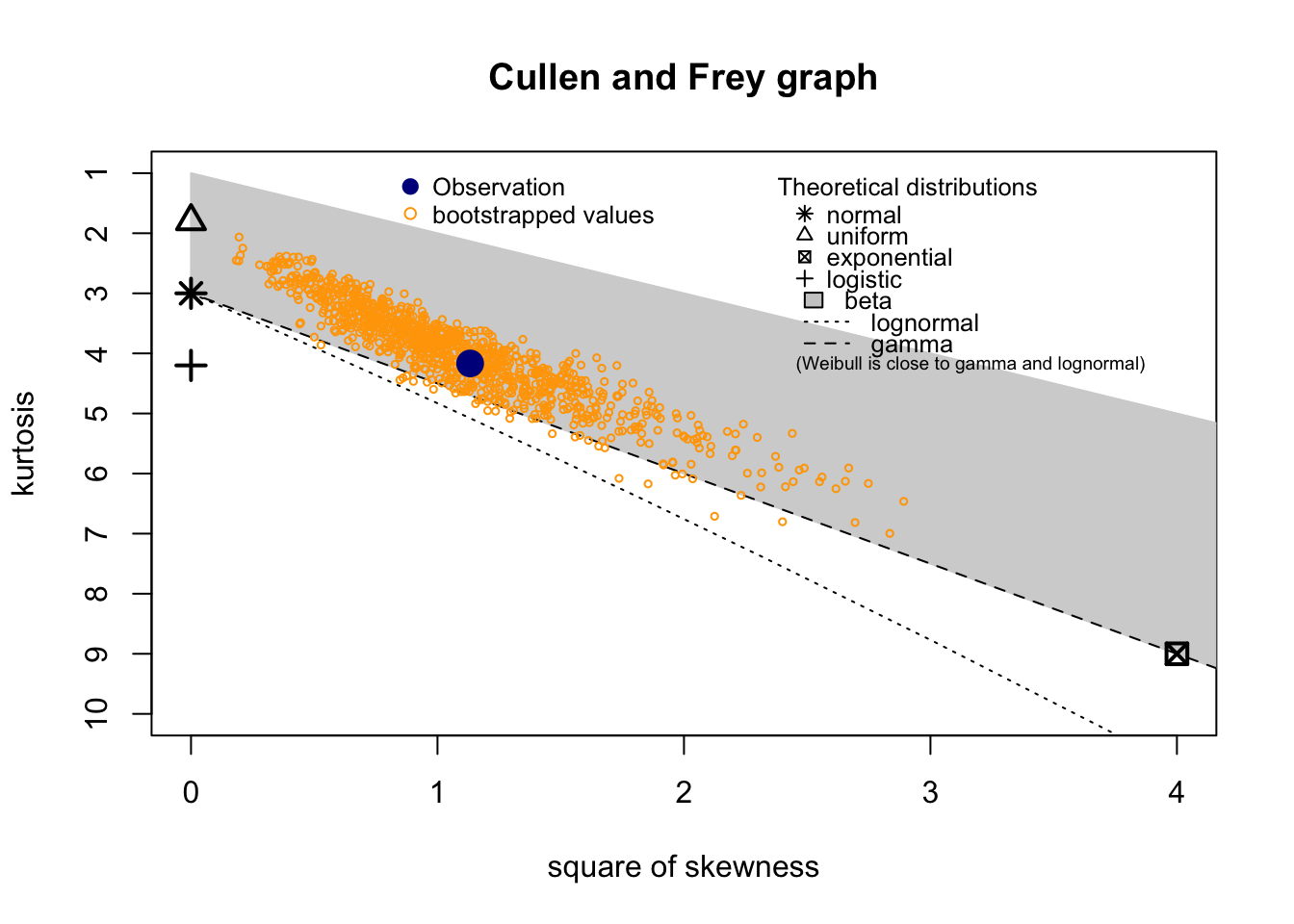
estimated skewness:  0.6162434 
estimated kurtosis:  6.394979

Normality & Homocedasticity

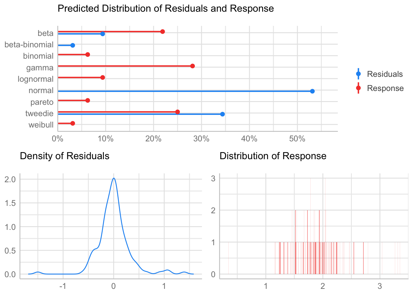
[1] "Variances homogeneity?"

Warning: Variances differ between groups (Bartlett Test, p = 0.000).

[1] "Normality?"

Warning: Non-normality of residuals detected (p < .001).

[1] "Normality, Random effects"

Group: zona:geo_parcela_nombre
(Intercept) OK: random effects appear as normally distributed (p = 0.918).

Model

Gamma

Fitting one lmer() model. [DONE]
Calculating p-values. [DONE]

Mixed Model Anova Table (Type 3 tests, KR-method)

Model: fe_percent ~ pre_post_quema * zona + (1 | zona:geo_parcela_nombre)
Data: df_model
               Effect     df    F p.value
1      pre_post_quema 1, 129 0.52    .473
2                zona   2, 9 0.69    .526
3 pre_post_quema:zona 2, 129 0.17    .845
---
Signif. codes:  0 '***' 0.001 '**' 0.01 '*' 0.05 '+' 0.1 ' ' 1

Post-hoc

$`emmeans of pre_post_quema`
 pre_post_quema emmean      SE  df asymp.LCL asymp.UCL
 0 Pre           0.549 0.00599 Inf     0.537     0.561
 1 Post          0.560 0.00818 Inf     0.544     0.576

Results are averaged over the levels of: zona 
Results are given on the inverse (not the response) scale. 
Confidence level used: 0.95 

$`pairwise differences of pre_post_quema`
 1              estimate      SE  df z.ratio p.value
 0 Pre - 1 Post  -0.0112 0.00566 Inf -1.979  0.0478 

Results are averaged over the levels of: zona 
Note: contrasts are still on the inverse scale

$`emmeans of zona`
 zona emmean      SE  df asymp.LCL asymp.UCL
 NP    0.526 0.00599 Inf     0.514     0.538
 P     0.607 0.00848 Inf     0.590     0.623
 PR    0.531 0.00846 Inf     0.514     0.547

Results are averaged over the levels of: pre_post_quema 
Results are given on the inverse (not the response) scale. 
Confidence level used: 0.95 

$`pairwise differences of zona`
 1       estimate      SE  df z.ratio p.value
 NP - P  -0.08067 0.00609 Inf -13.241 <.0001 
 NP - PR -0.00486 0.00608 Inf  -0.799 0.7036 
 P - PR   0.07581 0.00860 Inf   8.819 <.0001 

Results are averaged over the levels of: pre_post_quema 
Note: contrasts are still on the inverse scale 
P value adjustment: tukey method for comparing a family of 3 estimates

$`emmeans of pre_post_quema | zona`
zona = NP:
 pre_post_quema emmean      SE  df asymp.LCL asymp.UCL
 0 Pre           0.515 0.00543 Inf     0.504     0.526
 1 Post          0.537 0.00747 Inf     0.522     0.552

zona = P:
 pre_post_quema emmean      SE  df asymp.LCL asymp.UCL
 0 Pre           0.601 0.00768 Inf     0.586     0.616
 1 Post          0.612 0.01058 Inf     0.591     0.633

zona = PR:
 pre_post_quema emmean      SE  df asymp.LCL asymp.UCL
 0 Pre           0.530 0.00767 Inf     0.515     0.545
 1 Post          0.531 0.01054 Inf     0.511     0.552

Results are given on the inverse (not the response) scale. 
Confidence level used: 0.95 

$`pairwise differences of pre_post_quema | zona`
zona = NP:
 2              estimate      SE  df z.ratio p.value
 0 Pre - 1 Post -0.02193 0.00519 Inf -4.225  <.0001 

zona = P:
 2              estimate      SE  df z.ratio p.value
 0 Pre - 1 Post -0.01062 0.00737 Inf -1.442  0.1493 

zona = PR:
 2              estimate      SE  df z.ratio p.value
 0 Pre - 1 Post -0.00106 0.00732 Inf -0.144  0.8853 

Note: contrasts are still on the inverse scale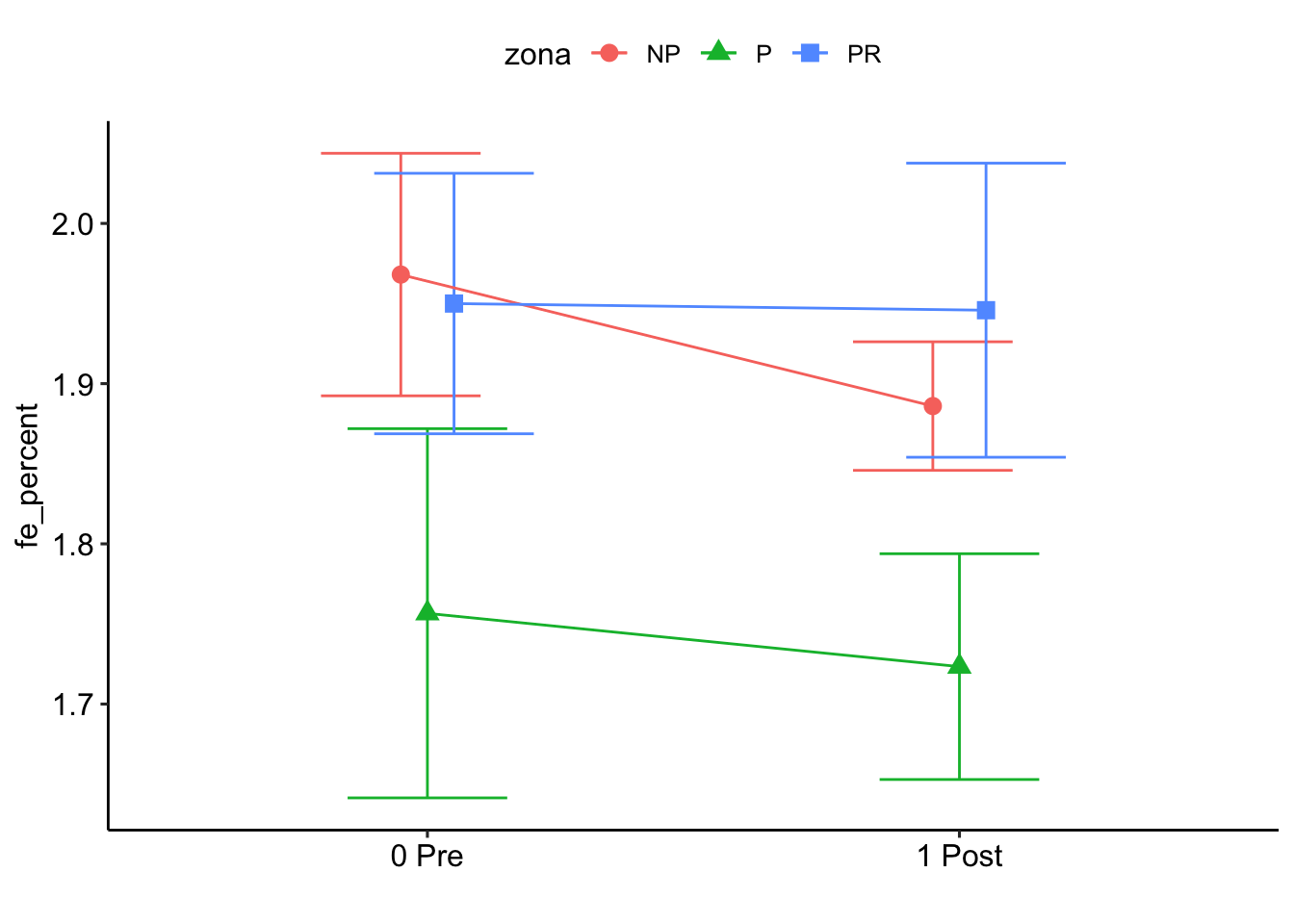

% K

Check distribution

summary statistics
------
min:  0.056   max:  1.74 
median:  0.4965 
mean:  0.5435972 
estimated sd:  0.2791576 
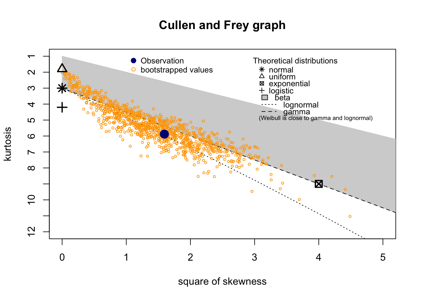
estimated skewness:  1.262402 
estimated kurtosis:  5.88111

Normality & Homocedasticity

[1] "Variances homogeneity?"

Warning: Variances differ between groups (Bartlett Test, p = 0.000).

[1] "Normality?"

Warning: Non-normality of residuals detected (p < .001).

[1] "Normality, Random effects"

Group: zona:geo_parcela_nombre
(Intercept) OK: random effects appear as normally distributed (p = 0.339).

Model

Gamma

Fitting one lmer() model. [DONE]
Calculating p-values. [DONE]

Mixed Model Anova Table (Type 3 tests, KR-method)

Model: k_percent ~ pre_post_quema * zona + (1 | zona:geo_parcela_nombre)
Data: df_model
               Effect     df      F p.value
1      pre_post_quema 1, 129   2.19    .141
2                zona   2, 9 6.73 *    .016
3 pre_post_quema:zona 2, 129   0.43    .651
---
Signif. codes:  0 '***' 0.001 '**' 0.01 '*' 0.05 '+' 0.1 ' ' 1

Post-hoc

$`emmeans of pre_post_quema`
 pre_post_quema emmean    SE  df asymp.LCL asymp.UCL
 0 Pre            2.13 0.168 Inf      1.80      2.46
 1 Post           2.37 0.173 Inf      2.03      2.71

Results are averaged over the levels of: zona 
Results are given on the inverse (not the response) scale. 
Confidence level used: 0.95 

$`pairwise differences of pre_post_quema`
 1              estimate    SE  df z.ratio p.value
 0 Pre - 1 Post   -0.243 0.107 Inf -2.275  0.0229 

Results are averaged over the levels of: zona 
Note: contrasts are still on the inverse scale

$`emmeans of zona`
 zona emmean    SE  df asymp.LCL asymp.UCL
 NP     2.01 0.273 Inf     1.472      2.54
 P      3.25 0.257 Inf     2.746      3.75
 PR     1.49 0.303 Inf     0.896      2.08

Results are averaged over the levels of: pre_post_quema 
Results are given on the inverse (not the response) scale. 
Confidence level used: 0.95 

$`pairwise differences of zona`
 1       estimate    SE  df z.ratio p.value
 NP - P    -1.242 0.372 Inf -3.339  0.0024 
 NP - PR    0.517 0.406 Inf  1.273  0.4106 
 P - PR     1.759 0.396 Inf  4.445  <.0001 

Results are averaged over the levels of: pre_post_quema 
Note: contrasts are still on the inverse scale 
P value adjustment: tukey method for comparing a family of 3 estimates

$`emmeans of pre_post_quema | zona`
zona = NP:
 pre_post_quema emmean    SE  df asymp.LCL asymp.UCL
 0 Pre            1.99 0.283 Inf     1.438      2.55
 1 Post           2.02 0.283 Inf     1.466      2.58

zona = P:
 pre_post_quema emmean    SE  df asymp.LCL asymp.UCL
 0 Pre            2.93 0.276 Inf     2.386      3.47
 1 Post           3.57 0.301 Inf     2.982      4.16

zona = PR:
 pre_post_quema emmean    SE  df asymp.LCL asymp.UCL
 0 Pre            1.46 0.307 Inf     0.860      2.06
 1 Post           1.52 0.308 Inf     0.914      2.12

Results are given on the inverse (not the response) scale. 
Confidence level used: 0.95 

$`pairwise differences of pre_post_quema | zona`
zona = NP:
 2              estimate    SE  df z.ratio p.value
 0 Pre - 1 Post  -0.0297 0.150 Inf -0.198  0.8433 

zona = P:
 2              estimate    SE  df z.ratio p.value
 0 Pre - 1 Post  -0.6437 0.263 Inf -2.444  0.0145 

zona = PR:
 2              estimate    SE  df z.ratio p.value
 0 Pre - 1 Post  -0.0556 0.104 Inf -0.536  0.5921 

Note: contrasts are still on the inverse scale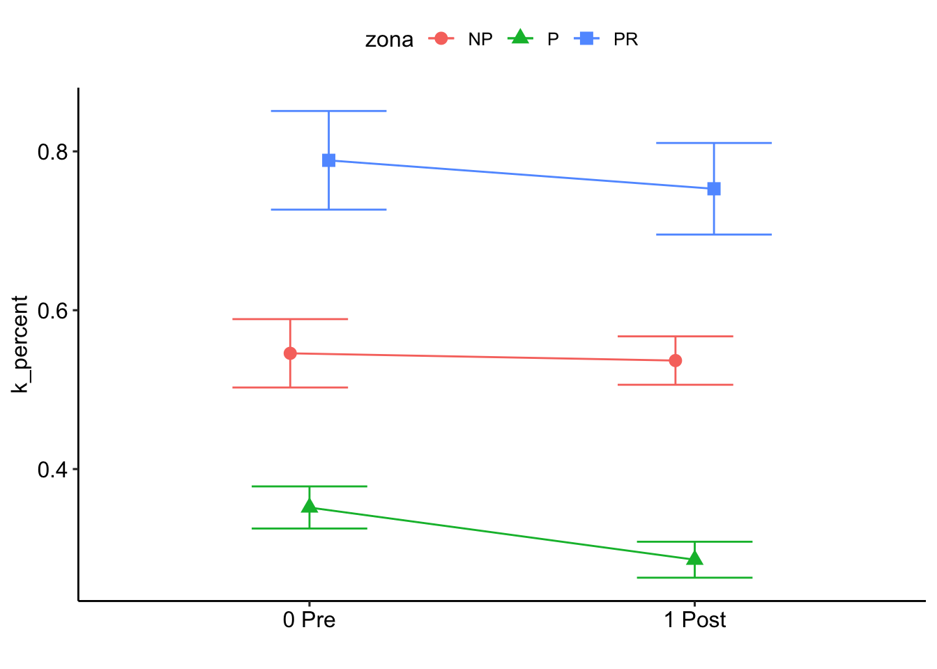

% Mg

Check distribution

summary statistics
------
min:  0.252   max:  4.59 
median:  1.4 
mean:  1.579299 
estimated sd:  0.8084862 
estimated skewness:  1.064159 
estimated kurtosis:  4.167461

Normality & Homocedasticity

[1] "Variances homogeneity?"

Warning: Variances differ between groups (Bartlett Test, p = 0.000).

[1] "Normality?"

Warning: Non-normality of residuals detected (p < .001).

[1] "Normality, Random effects"

Group: zona:geo_parcela_nombre
(Intercept) OK: random effects appear as normally distributed (p = 0.525).

Model

Gamma

Fitting one lmer() model. [DONE]
Calculating p-values. [DONE]

Mixed Model Anova Table (Type 3 tests, KR-method)

Model: mg_percent ~ pre_post_quema * zona + (1 | zona:geo_parcela_nombre)
Data: df_model
               Effect     df      F p.value
1      pre_post_quema 1, 129   1.37    .245
2                zona   2, 9 3.05 +    .097
3 pre_post_quema:zona 2, 129   0.84    .434
---
Signif. codes:  0 '***' 0.001 '**' 0.01 '*' 0.05 '+' 0.1 ' ' 1

Post-hoc

$`emmeans of pre_post_quema`
 pre_post_quema emmean     SE  df asymp.LCL asymp.UCL
 0 Pre           0.784 0.0807 Inf     0.625     0.942
 1 Post          0.749 0.0803 Inf     0.592     0.907

Results are averaged over the levels of: zona 
Results are given on the inverse (not the response) scale. 
Confidence level used: 0.95 

$`pairwise differences of pre_post_quema`
 1              estimate     SE  df z.ratio p.value
 0 Pre - 1 Post   0.0345 0.0371 Inf 0.929   0.3528 

Results are averaged over the levels of: zona 
Note: contrasts are still on the inverse scale

$`emmeans of zona`
 zona emmean    SE  df asymp.LCL asymp.UCL
 NP    0.759 0.133 Inf     0.498      1.02
 P     0.992 0.125 Inf     0.747      1.24
 PR    0.548 0.144 Inf     0.265      0.83

Results are averaged over the levels of: pre_post_quema 
Results are given on the inverse (not the response) scale. 
Confidence level used: 0.95 

$`pairwise differences of zona`
 1       estimate    SE  df z.ratio p.value
 NP - P    -0.233 0.181 Inf -1.286  0.4032 
 NP - PR    0.212 0.196 Inf  1.080  0.5264 
 P - PR     0.445 0.190 Inf  2.341  0.0504 

Results are averaged over the levels of: pre_post_quema 
Note: contrasts are still on the inverse scale 
P value adjustment: tukey method for comparing a family of 3 estimates

$`emmeans of pre_post_quema | zona`
zona = NP:
 pre_post_quema emmean    SE  df asymp.LCL asymp.UCL
 0 Pre           0.807 0.137 Inf     0.538     1.076
 1 Post          0.711 0.135 Inf     0.446     0.977

zona = P:
 pre_post_quema emmean    SE  df asymp.LCL asymp.UCL
 0 Pre           0.988 0.132 Inf     0.730     1.247
 1 Post          0.996 0.132 Inf     0.737     1.255

zona = PR:
 pre_post_quema emmean    SE  df asymp.LCL asymp.UCL
 0 Pre           0.555 0.146 Inf     0.269     0.841
 1 Post          0.540 0.146 Inf     0.255     0.826

Results are given on the inverse (not the response) scale. 
Confidence level used: 0.95 

$`pairwise differences of pre_post_quema | zona`
zona = NP:
 2              estimate     SE  df z.ratio p.value
 0 Pre - 1 Post  0.09632 0.0566 Inf  1.702  0.0887 

zona = P:
 2              estimate     SE  df z.ratio p.value
 0 Pre - 1 Post -0.00743 0.0841 Inf -0.088  0.9296 

zona = PR:
 2              estimate     SE  df z.ratio p.value
 0 Pre - 1 Post  0.01456 0.0461 Inf  0.316  0.7523 

Note: contrasts are still on the inverse scale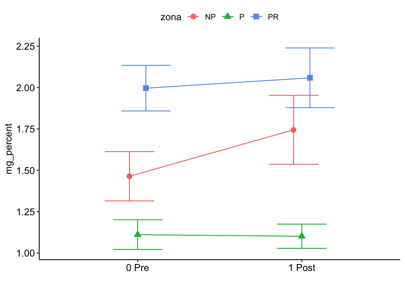

C/N

Check distribution

summary statistics
------
min:  14.20907   max:  116.0373 
median:  34.20672 
mean:  39.50944 
estimated sd:  19.74075 
estimated skewness:  1.645355 
estimated kurtosis:  6.246139

Normality & Homocedasticity

[1] "Variances homogeneity?"

OK: Variances in each of the groups are the same (Bartlett Test, p = 0.136).

[1] "Normality?"

Warning: Non-normality of residuals detected (p < .001).

[1] "Normality, Random effects"

Group: zona:geo_parcela_nombre
(Intercept) OK: random effects appear as normally distributed (p = 0.614).

Model

Gamma

Fitting one lmer() model. [DONE]
Calculating p-values. [DONE]

Mixed Model Anova Table (Type 3 tests, KR-method)

Model: c_n ~ pre_post_quema * zona + (1 | zona:geo_parcela_nombre)
Data: df_model
               Effect     df    F p.value
1      pre_post_quema 1, 129 0.32    .574
2                zona   2, 9 0.43    .663
3 pre_post_quema:zona 2, 129 0.42    .659
---
Signif. codes:  0 '***' 0.001 '**' 0.01 '*' 0.05 '+' 0.1 ' ' 1

Post-hoc

$`emmeans of pre_post_quema`
 pre_post_quema emmean      SE  df asymp.LCL asymp.UCL
 0 Pre          0.0269 0.00248 Inf    0.0221    0.0318
 1 Post         0.0281 0.00250 Inf    0.0232    0.0330

Results are averaged over the levels of: zona 
Results are given on the inverse (not the response) scale. 
Confidence level used: 0.95 

$`pairwise differences of pre_post_quema`
 1              estimate     SE  df z.ratio p.value
 0 Pre - 1 Post -0.00119 0.0016 Inf -0.743  0.4574 

Results are averaged over the levels of: zona 
Note: contrasts are still on the inverse scale

$`emmeans of zona`
 zona emmean      SE  df asymp.LCL asymp.UCL
 NP   0.0301 0.00398 Inf    0.0223    0.0379
 P    0.0275 0.00403 Inf    0.0196    0.0354
 PR   0.0249 0.00402 Inf    0.0171    0.0328

Results are averaged over the levels of: pre_post_quema 
Results are given on the inverse (not the response) scale. 
Confidence level used: 0.95 

$`pairwise differences of zona`
 1       estimate      SE  df z.ratio p.value
 NP - P   0.00257 0.00559 Inf 0.459   0.8904 
 NP - PR  0.00514 0.00562 Inf 0.915   0.6311 
 P - PR   0.00257 0.00566 Inf 0.455   0.8923 

Results are averaged over the levels of: pre_post_quema 
Note: contrasts are still on the inverse scale 
P value adjustment: tukey method for comparing a family of 3 estimates

$`emmeans of pre_post_quema | zona`
zona = NP:
 pre_post_quema emmean      SE  df asymp.LCL asymp.UCL
 0 Pre          0.0290 0.00422 Inf    0.0207    0.0373
 1 Post         0.0312 0.00431 Inf    0.0227    0.0396

zona = P:
 pre_post_quema emmean      SE  df asymp.LCL asymp.UCL
 0 Pre          0.0263 0.00421 Inf    0.0180    0.0345
 1 Post         0.0288 0.00429 Inf    0.0204    0.0372

zona = PR:
 pre_post_quema emmean      SE  df asymp.LCL asymp.UCL
 0 Pre          0.0255 0.00424 Inf    0.0172    0.0338
 1 Post         0.0244 0.00420 Inf    0.0162    0.0326

Results are given on the inverse (not the response) scale. 
Confidence level used: 0.95 

$`pairwise differences of pre_post_quema | zona`
zona = NP:
 2              estimate      SE  df z.ratio p.value
 0 Pre - 1 Post -0.00215 0.00305 Inf -0.706  0.4803 

zona = P:
 2              estimate      SE  df z.ratio p.value
 0 Pre - 1 Post -0.00252 0.00269 Inf -0.939  0.3479 

zona = PR:
 2              estimate      SE  df z.ratio p.value
 0 Pre - 1 Post  0.00111 0.00255 Inf  0.435  0.6635 

Note: contrasts are still on the inverse scale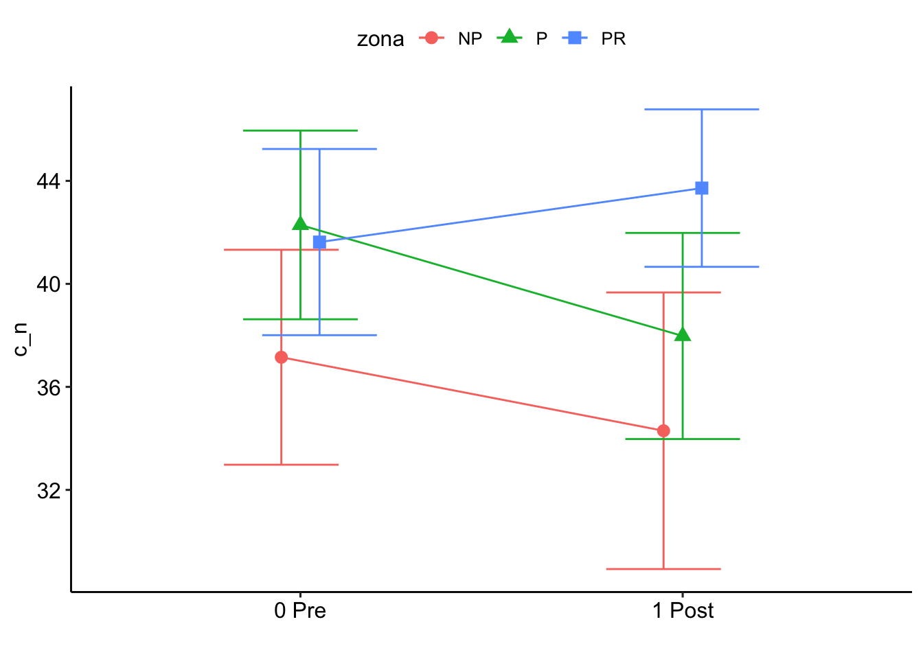

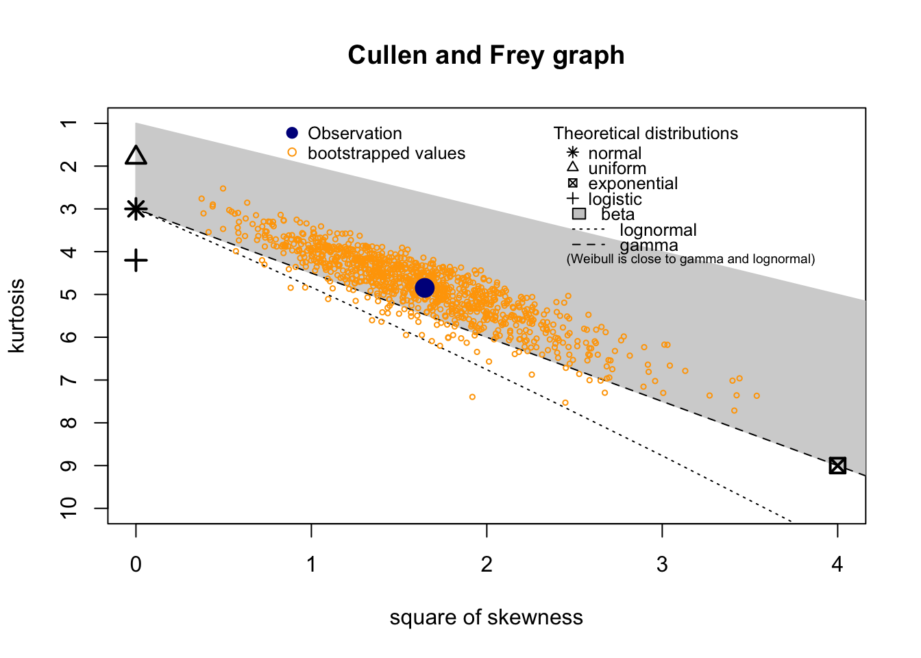
P

Check distribution

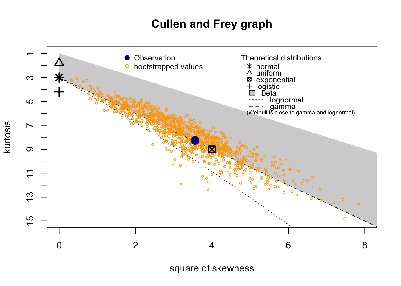
summary statistics
------
min:  1   max:  17 
median:  4.5 
mean:  5.116667 
estimated sd:  2.43368 
estimated skewness:  1.886353 
estimated kurtosis:  8.270509

Normality & Homocedasticity

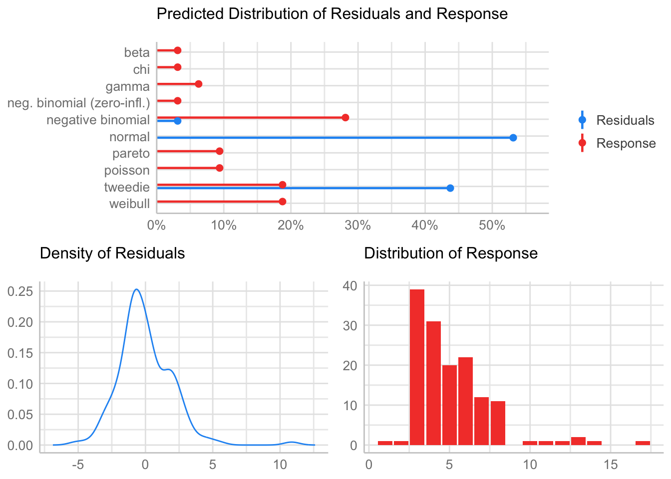
[1] "Variances homogeneity?"

Warning: Variances differ between groups (Bartlett Test, p = 0.000).

[1] "Normality?"

Warning: Non-normality of residuals detected (p < .001).

[1] "Normality, Random effects"

Group: zona:geo_parcela_nombre
(Intercept) Warning: Non-normality of random effects detected (p = 0.007).

Model

Negative Binomial

Fitting one lmer() model. [DONE]
Calculating p-values. [DONE]

Mixed Model Anova Table (Type 3 tests, KR-method)

Model: p ~ pre_post_quema * zona + (1 | zona:geo_parcela_nombre)
Data: df_model
               Effect     df       F p.value
1      pre_post_quema 1, 129  3.20 +    .076
2                zona   2, 9  3.81 +    .063
3 pre_post_quema:zona 2, 129 4.88 **    .009
---
Signif. codes:  0 '***' 0.001 '**' 0.01 '*' 0.05 '+' 0.1 ' ' 1

Post-hoc

$`emmeans of pre_post_quema`
 pre_post_quema emmean     SE  df asymp.LCL asymp.UCL
 0 Pre            1.53 0.0628 Inf      1.40      1.65
 1 Post           1.68 0.0588 Inf      1.57      1.80

Results are averaged over the levels of: zona 
Results are given on the log (not the response) scale. 
Confidence level used: 0.95 

$`pairwise differences of pre_post_quema`
 1              estimate     SE  df z.ratio p.value
 0 Pre - 1 Post   -0.156 0.0744 Inf -2.103  0.0355 

Results are averaged over the levels of: zona 
Results are given on the log (not the response) scale.

$`emmeans of zona`
 zona emmean     SE  df asymp.LCL asymp.UCL
 NP     1.52 0.0844 Inf      1.35      1.69
 P      1.46 0.0870 Inf      1.29      1.64
 PR     1.83 0.0776 Inf      1.68      1.98

Results are averaged over the levels of: pre_post_quema 
Results are given on the log (not the response) scale. 
Confidence level used: 0.95 

$`pairwise differences of zona`
 1       estimate    SE  df z.ratio p.value
 NP - P    0.0548 0.121 Inf  0.451  0.8938 
 NP - PR  -0.3116 0.114 Inf -2.734  0.0172 
 P - PR   -0.3664 0.116 Inf -3.147  0.0047 

Results are averaged over the levels of: pre_post_quema 
Results are given on the log (not the response) scale. 
P value adjustment: tukey method for comparing a family of 3 estimates

$`emmeans of pre_post_quema | zona`
zona = NP:
 pre_post_quema emmean     SE  df asymp.LCL asymp.UCL
 0 Pre            1.34 0.1122 Inf      1.12      1.56
 1 Post           1.70 0.0998 Inf      1.50      1.90

zona = P:
 pre_post_quema emmean     SE  df asymp.LCL asymp.UCL
 0 Pre            1.34 0.1165 Inf      1.11      1.57
 1 Post           1.59 0.1053 Inf      1.38      1.79

zona = PR:
 pre_post_quema emmean     SE  df asymp.LCL asymp.UCL
 0 Pre            1.90 0.0936 Inf      1.72      2.08
 1 Post           1.76 0.0989 Inf      1.57      1.96

Results are given on the log (not the response) scale. 
Confidence level used: 0.95 

$`pairwise differences of pre_post_quema | zona`
zona = NP:
 2              estimate    SE  df z.ratio p.value
 0 Pre - 1 Post   -0.361 0.129 Inf -2.808  0.0050 

zona = P:
 2              estimate    SE  df z.ratio p.value
 0 Pre - 1 Post   -0.247 0.138 Inf -1.790  0.0734 

zona = PR:
 2              estimate    SE  df z.ratio p.value
 0 Pre - 1 Post    0.139 0.114 Inf  1.217  0.2235 

Results are given on the log (not the response) scale.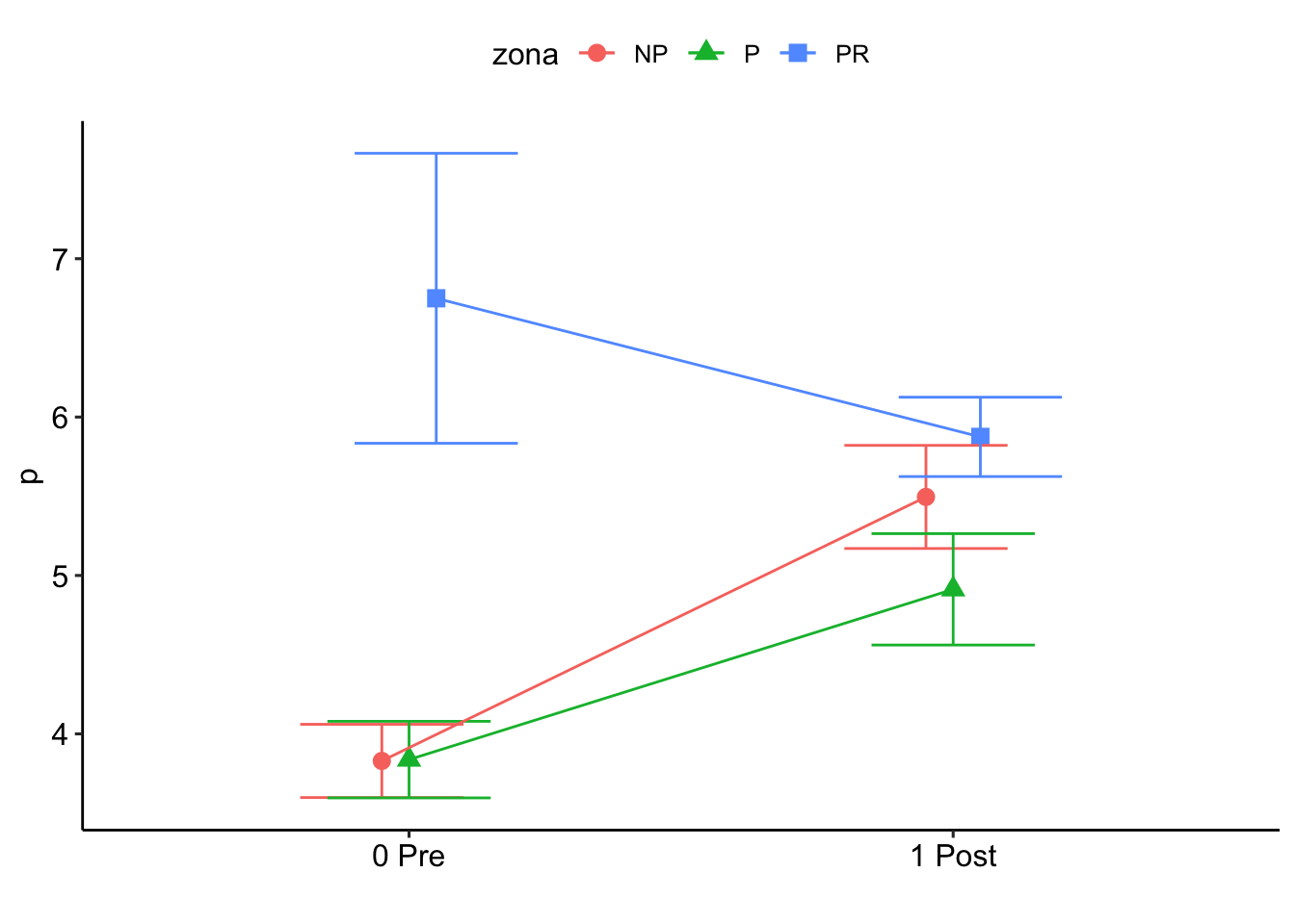

MO

Check distribution

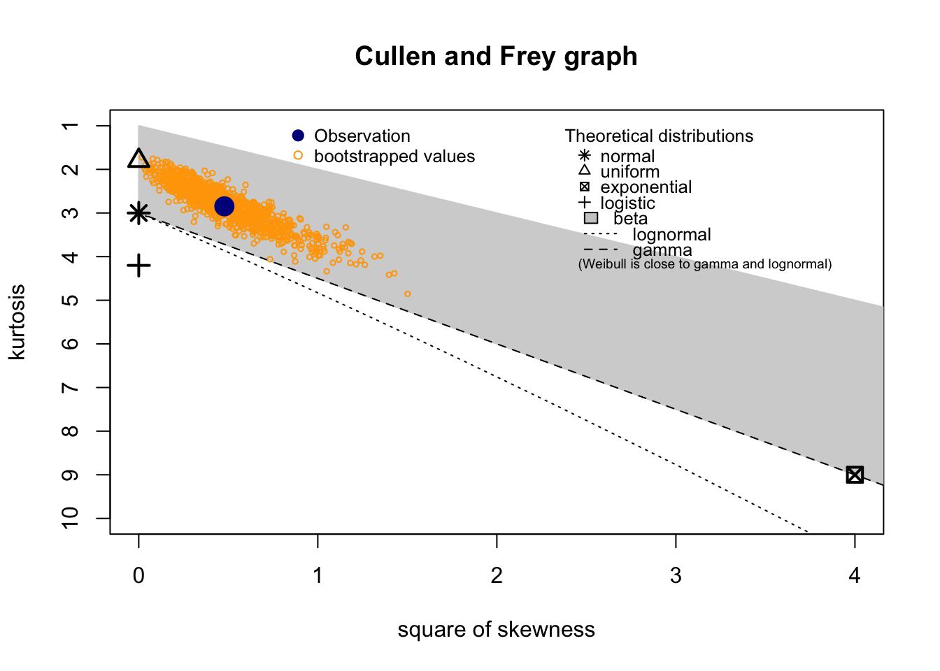
summary statistics
------
min:  0.44   max:  12.91 
median:  4.4 
mean:  4.737431 
estimated sd:  2.507076 
estimated skewness:  0.6914957 
estimated kurtosis:  2.846614

Normality & Homocedasticity

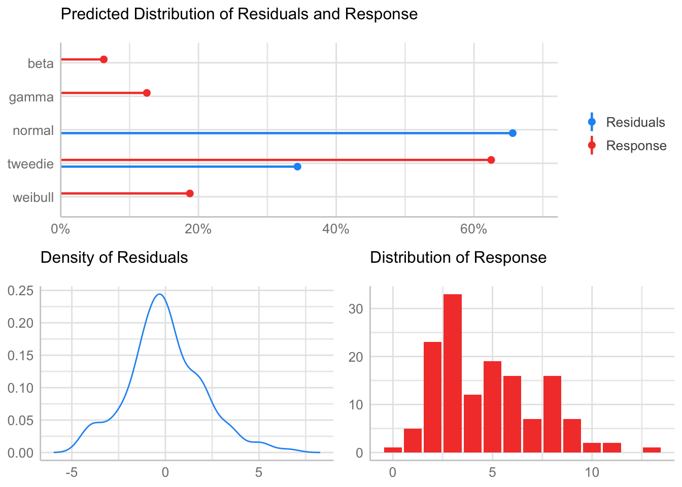
[1] "Variances homogeneity?"

Warning: Variances differ between groups (Bartlett Test, p = 0.000).

[1] "Normality?"

Warning: Non-normality of residuals detected (p = 0.036).

[1] "Normality, Random effects"

Group: zona:geo_parcela_nombre
(Intercept) OK: random effects appear as normally distributed (p = 0.837).

Model

Gamma

Fitting one lmer() model. [DONE]
Calculating p-values. [DONE]

Mixed Model Anova Table (Type 3 tests, KR-method)

Model: mo ~ pre_post_quema * zona + (1 | zona:geo_parcela_nombre)
Data: df_model
               Effect     df         F p.value
1      pre_post_quema 1, 129      1.35    .247
2                zona   2, 9 20.37 ***   <.001
3 pre_post_quema:zona 2, 129      1.04    .357
---
Signif. codes:  0 '***' 0.001 '**' 0.01 '*' 0.05 '+' 0.1 ' ' 1

Post-hoc

$`emmeans of pre_post_quema`
 pre_post_quema emmean     SE  df asymp.LCL asymp.UCL
 0 Pre           0.244 0.0152 Inf     0.215     0.274
 1 Post          0.233 0.0149 Inf     0.203     0.262

Results are averaged over the levels of: zona 
Results are given on the inverse (not the response) scale. 
Confidence level used: 0.95 

$`pairwise differences of pre_post_quema`
 1              estimate     SE  df z.ratio p.value
 0 Pre - 1 Post   0.0117 0.0177 Inf 0.660   0.5094 

Results are averaged over the levels of: zona 
Note: contrasts are still on the inverse scale

$`emmeans of zona`
 zona emmean     SE  df asymp.LCL asymp.UCL
 NP    0.194 0.0186 Inf     0.157     0.230
 P     0.168 0.0176 Inf     0.133     0.202
 PR    0.354 0.0254 Inf     0.305     0.404

Results are averaged over the levels of: pre_post_quema 
Results are given on the inverse (not the response) scale. 
Confidence level used: 0.95 

$`pairwise differences of zona`
 1       estimate     SE  df z.ratio p.value
 NP - P    0.0261 0.0253 Inf  1.034  0.5556 
 NP - PR  -0.1608 0.0312 Inf -5.156  <.0001 
 P - PR   -0.1870 0.0307 Inf -6.084  <.0001 

Results are averaged over the levels of: pre_post_quema 
Note: contrasts are still on the inverse scale 
P value adjustment: tukey method for comparing a family of 3 estimates

$`emmeans of pre_post_quema | zona`
zona = NP:
 pre_post_quema emmean     SE  df asymp.LCL asymp.UCL
 0 Pre           0.213 0.0231 Inf     0.168     0.258
 1 Post          0.174 0.0206 Inf     0.134     0.215

zona = P:
 pre_post_quema emmean     SE  df asymp.LCL asymp.UCL
 0 Pre           0.170 0.0204 Inf     0.130     0.210
 1 Post          0.165 0.0201 Inf     0.126     0.205

zona = PR:
 pre_post_quema emmean     SE  df asymp.LCL asymp.UCL
 0 Pre           0.350 0.0330 Inf     0.286     0.415
 1 Post          0.359 0.0337 Inf     0.293     0.425

Results are given on the inverse (not the response) scale. 
Confidence level used: 0.95 

$`pairwise differences of pre_post_quema | zona`
zona = NP:
 2              estimate     SE  df z.ratio p.value
 0 Pre - 1 Post  0.03837 0.0233 Inf  1.648  0.0993 

zona = P:
 2              estimate     SE  df z.ratio p.value
 0 Pre - 1 Post  0.00480 0.0201 Inf  0.239  0.8111 

zona = PR:
 2              estimate     SE  df z.ratio p.value
 0 Pre - 1 Post -0.00816 0.0432 Inf -0.189  0.8502 

Note: contrasts are still on the inverse scale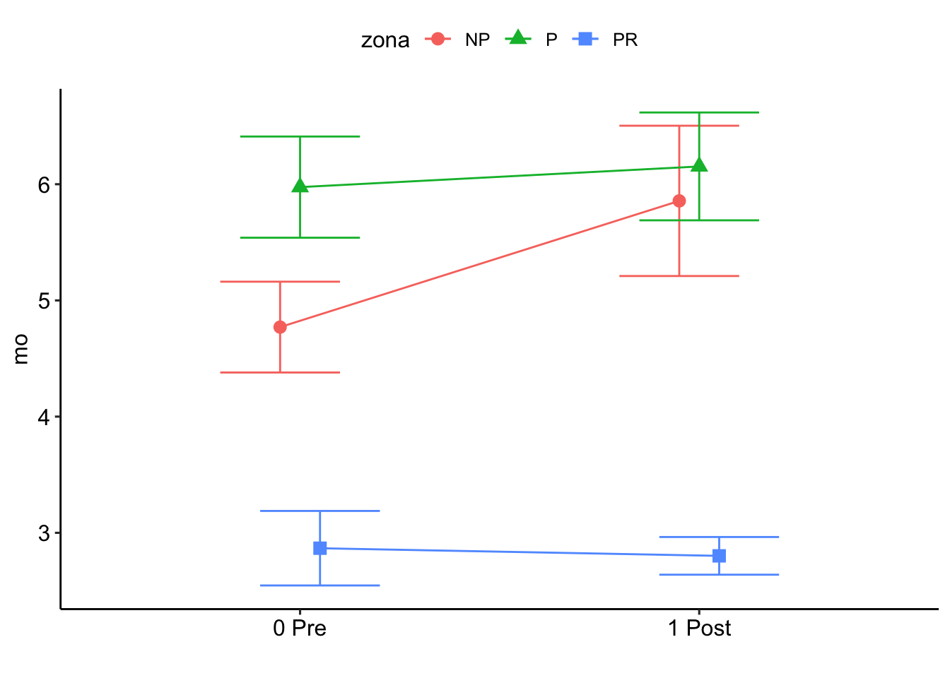

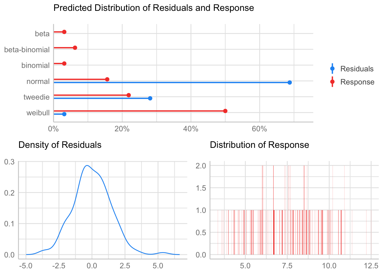
% N

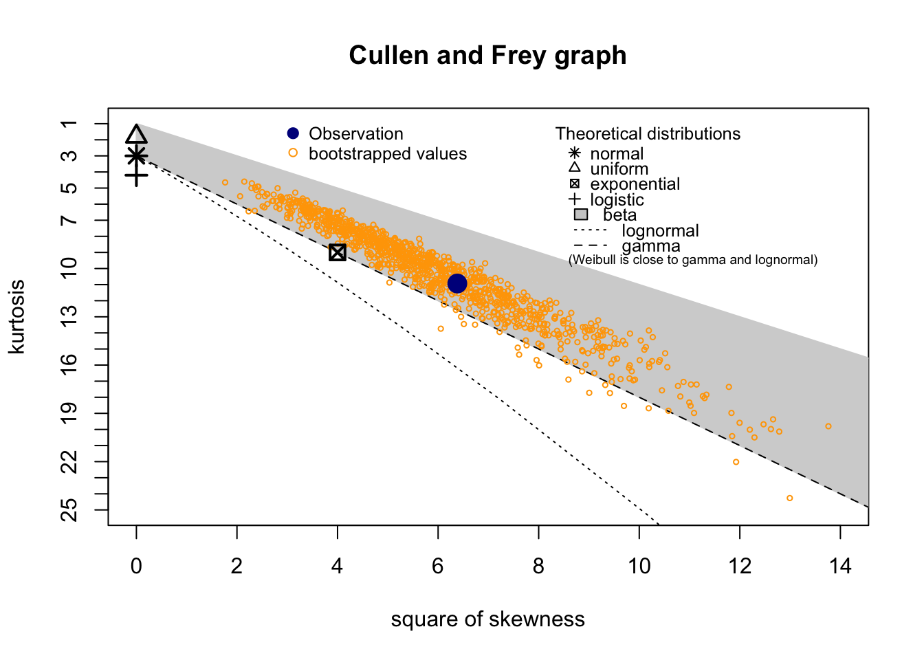
Check distribution

summary statistics
------
min:  0.0427   max:  0.634455 
median:  0.2104425 
mean:  0.2299281 
estimated sd:  0.1176054 
estimated skewness:  1.283039 
estimated kurtosis:  4.846892

Normality & Homocedasticity

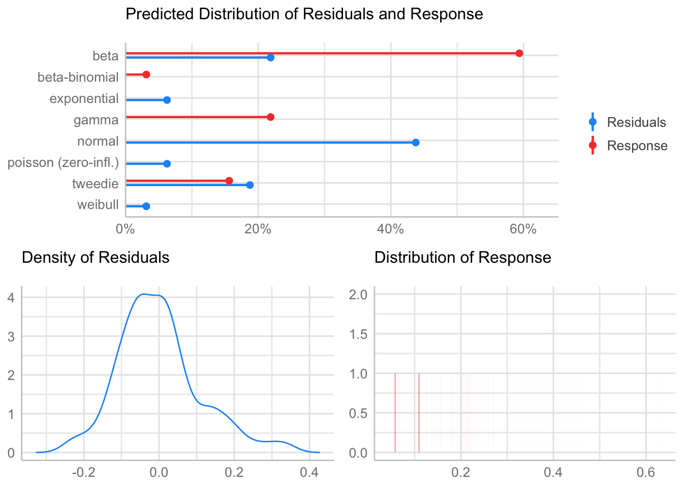
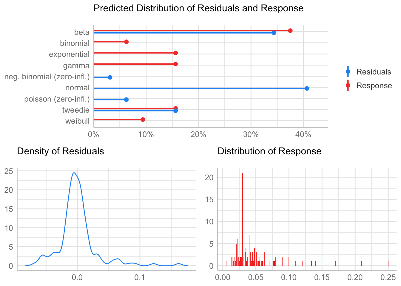
[1] "Variances homogeneity?"

Warning: Variances differ between groups (Bartlett Test, p = 0.000).

[1] "Normality?"

Warning: Non-normality of residuals detected (p < .001).

Model

Beta (glmmADBM)
Beta glmmTMB

Post-hoc

$`emmeans of pre_post_quema`
 pre_post_quema emmean     SE  df lower.CL upper.CL
 0 Pre           -1.31 0.0710 136    -1.45   -1.171
 1 Post          -1.10 0.0678 136    -1.24   -0.968

Results are averaged over the levels of: zona 
Results are given on the logit (not the response) scale. 
Confidence level used: 0.95 

$`pairwise differences of pre_post_quema`
 1              estimate     SE  df t.ratio p.value
 0 Pre - 1 Post    -0.21 0.0968 136 -2.170  0.0318 

Results are averaged over the levels of: zona 
Results are given on the log odds ratio (not the response) scale.

$`emmeans of zona`
 zona emmean     SE  df lower.CL upper.CL
 NP    -1.11 0.0827 136    -1.27   -0.947
 P     -1.12 0.0828 136    -1.28   -0.953
 PR    -1.39 0.0882 136    -1.57   -1.219

Results are averaged over the levels of: pre_post_quema 
Results are given on the logit (not the response) scale. 
Confidence level used: 0.95 

$`pairwise differences of zona`
 1       estimate    SE  df t.ratio p.value
 NP - P   0.00552 0.116 136 0.048   0.9988 
 NP - PR  0.28266 0.120 136 2.362   0.0510 
 P - PR   0.27714 0.120 136 2.315   0.0571 

Results are averaged over the levels of: pre_post_quema 
Results are given on the log odds ratio (not the response) scale. 
P value adjustment: tukey method for comparing a family of 3 estimates

$`emmeans of pre_post_quema | zona`
zona = NP:
 pre_post_quema emmean    SE  df lower.CL upper.CL
 0 Pre          -1.282 0.121 136    -1.52   -1.043
 1 Post         -0.940 0.112 136    -1.16   -0.718

zona = P:
 pre_post_quema emmean    SE  df lower.CL upper.CL
 0 Pre          -1.269 0.120 136    -1.51   -1.031
 1 Post         -0.964 0.113 136    -1.19   -0.741

zona = PR:
 pre_post_quema emmean    SE  df lower.CL upper.CL
 0 Pre          -1.384 0.124 136    -1.63   -1.140
 1 Post         -1.403 0.124 136    -1.65   -1.157

Results are given on the logit (not the response) scale. 
Confidence level used: 0.95 

$`pairwise differences of pre_post_quema | zona`
zona = NP:
 2              estimate    SE  df t.ratio p.value
 0 Pre - 1 Post  -0.3425 0.164 136 -2.086  0.0388 

zona = P:
 2              estimate    SE  df t.ratio p.value
 0 Pre - 1 Post  -0.3055 0.164 136 -1.860  0.0650 

zona = PR:
 2              estimate    SE  df t.ratio p.value
 0 Pre - 1 Post   0.0182 0.174 136  0.104  0.9171 

Results are given on the log odds ratio (not the response) scale.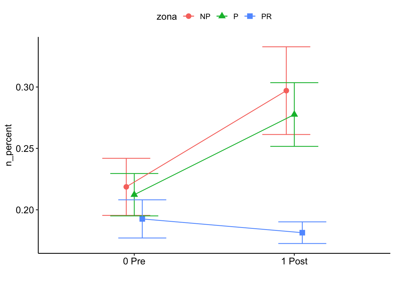

% Na

Check distribution

summary statistics
------
min:  0.005   max:  0.25 
median:  0.0355 
mean:  0.04798611 
estimated sd:  0.0382072 
estimated skewness:  2.52624 
estimated kurtosis:  10.93139

Normality & Homocedasticity

[1] "Variances homogeneity?"

Warning: Variances differ between groups (Bartlett Test, p = 0.000).

[1] "Normality?"

Warning: Non-normality of residuals detected (p < .001).

[1] "Normality, Random effects"

Group: zona:geo_parcela_nombre
(Intercept) OK: random effects appear as normally distributed (p = 0.952).

Model

Beta (glmmADBM)

Analysis of Deviance Table (Type II tests)

Response: na_percent
                    Df  Chisq Pr(>Chisq)  
pre_post_quema       1 0.0675    0.79498  
zona                 2 5.0992    0.07811 .
pre_post_quema:zona  2 0.1864    0.91101  
---
Signif. codes:  0 '***' 0.001 '**' 0.01 '*' 0.05 '.' 0.1 ' ' 1

Fitting one lmer() model. [DONE]
Calculating p-values. [DONE]

Mixed Model Anova Table (Type 3 tests, KR-method)

Model: na_percent ~ pre_post_quema * zona + (1 | zona:geo_parcela_nombre)
Data: df_model
               Effect     df    F p.value
1      pre_post_quema 1, 129 0.42    .518
2                zona   2, 9 2.82    .112
3 pre_post_quema:zona 2, 129 0.18    .836
---
Signif. codes:  0 '***' 0.001 '**' 0.01 '*' 0.05 '+' 0.1 ' ' 1

Beta glmmTMB

Analysis of Deviance Table (Type II Wald chisquare tests)

Response: na_percent
                      Chisq Df Pr(>Chisq)   
pre_post_quema       0.6972  1   0.403726   
zona                11.9551  2   0.002535 **
pre_post_quema:zona  0.2408  2   0.886558   
---
Signif. codes:  0 '***' 0.001 '**' 0.01 '*' 0.05 '.' 0.1 ' ' 1

Post-hoc

$`emmeans of pre_post_quema`
 pre_post_quema emmean     SE  df lower.CL upper.CL
 0 Pre           -3.00 0.0916 136    -3.18    -2.82
 1 Post          -3.08 0.0934 136    -3.26    -2.90

Results are averaged over the levels of: zona 
Results are given on the logit (not the response) scale. 
Confidence level used: 0.95 

$`pairwise differences of pre_post_quema`
 1              estimate     SE  df t.ratio p.value
 0 Pre - 1 Post    0.082 0.0891 136 0.920   0.3593 

Results are averaged over the levels of: zona 
Results are given on the log odds ratio (not the response) scale.

$`emmeans of zona`
 zona emmean    SE  df lower.CL upper.CL
 NP    -2.88 0.134 136    -3.15    -2.61
 P     -3.43 0.146 136    -3.72    -3.15
 PR    -2.80 0.133 136    -3.07    -2.54

Results are averaged over the levels of: pre_post_quema 
Results are given on the logit (not the response) scale. 
Confidence level used: 0.95 

$`pairwise differences of zona`
 1       estimate    SE  df t.ratio p.value
 NP - P    0.5523 0.196 136  2.816  0.0153 
 NP - PR  -0.0772 0.188 136 -0.411  0.9113 
 P - PR   -0.6295 0.195 136 -3.224  0.0045 

Results are averaged over the levels of: pre_post_quema 
Results are given on the log odds ratio (not the response) scale. 
P value adjustment: tukey method for comparing a family of 3 estimates

$`emmeans of pre_post_quema | zona`
zona = NP:
 pre_post_quema emmean    SE  df lower.CL upper.CL
 0 Pre           -2.86 0.152 136    -3.16    -2.56
 1 Post          -2.91 0.154 136    -3.21    -2.60

zona = P:
 pre_post_quema emmean    SE  df lower.CL upper.CL
 0 Pre           -3.36 0.168 136    -3.69    -3.03
 1 Post          -3.51 0.173 136    -3.85    -3.17

zona = PR:
 pre_post_quema emmean    SE  df lower.CL upper.CL
 0 Pre           -2.78 0.150 136    -3.08    -2.48
 1 Post          -2.83 0.151 136    -3.13    -2.53

Results are given on the logit (not the response) scale. 
Confidence level used: 0.95 

$`pairwise differences of pre_post_quema | zona`
zona = NP:
 2              estimate    SE  df t.ratio p.value
 0 Pre - 1 Post   0.0499 0.144 136 0.345   0.7303 

zona = P:
 2              estimate    SE  df t.ratio p.value
 0 Pre - 1 Post   0.1486 0.177 136 0.837   0.4039 

zona = PR:
 2              estimate    SE  df t.ratio p.value
 0 Pre - 1 Post   0.0475 0.139 136 0.343   0.7321 

Results are given on the log odds ratio (not the response) scale.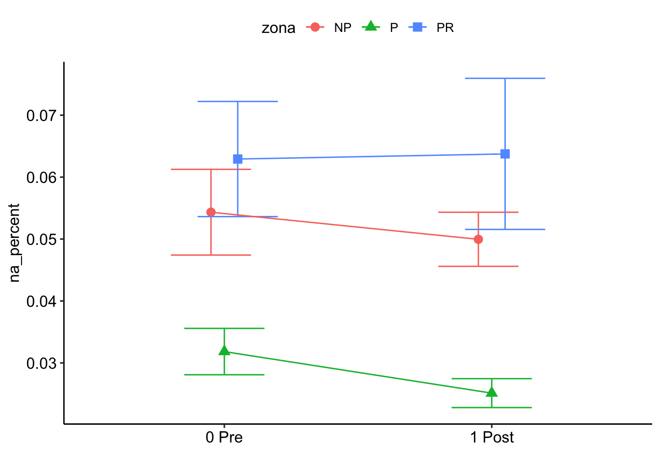

NH4

prepara datos

              zona
pre_post_quema NP  P
        0 Pre  24 24
        1 Post 24 23

# A tibble: 4 x 4
# Groups:   zona [2]
  zona  pre_post_quema N.nh4 N.no3
  <fct> <fct>          <int> <int>
1 NP    0 Pre             24    24
2 NP    1 Post            24    24
3 P     0 Pre             24    24
4 P     1 Post            23    23

Check distribution

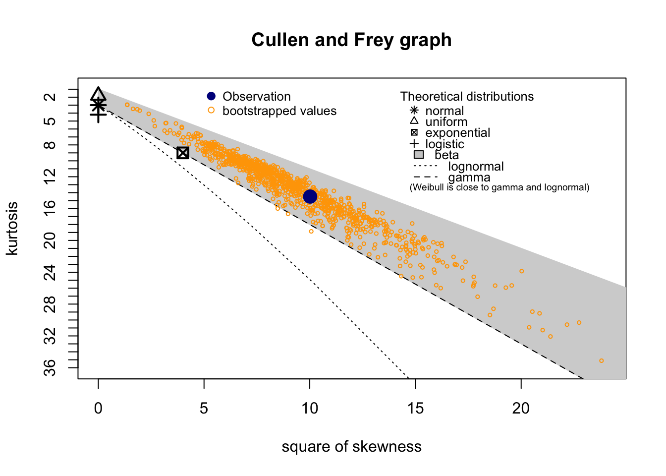
summary statistics
------
min:  0.258   max:  21.312 
median:  0.712 
mean:  2.315116 
estimated sd:  3.686985 
estimated skewness:  3.16529 
estimated kurtosis:  14.49165

Normality & Homocedasticity

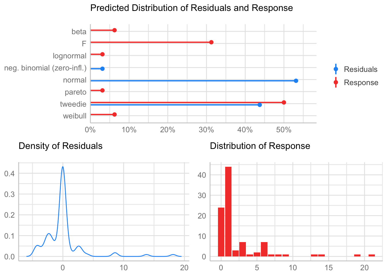
[1] "Variances homogeneity?"

Warning: Variances differ between groups (Bartlett Test, p = 0.000).

[1] "Normality?"

Warning: Non-normality of residuals detected (p < .001).

Model

Gamma

Fitting one lmer() model. [DONE]
Calculating p-values. [DONE]

Mixed Model Anova Table (Type 3 tests, KR-method)

Model: n_nh4 ~ pre_post_quema * zona + (1 | zona:geo_parcela_nombre)
Data: df_model
               Effect       df         F p.value
1      pre_post_quema 1, 85.12 26.17 ***   <.001
2                zona  1, 5.99      1.58    .256
3 pre_post_quema:zona 1, 85.12      1.72    .193
---
Signif. codes:  0 '***' 0.001 '**' 0.01 '*' 0.05 '+' 0.1 ' ' 1

Post-hoc

$`emmeans of pre_post_quema`
 pre_post_quema emmean     SE  df asymp.LCL asymp.UCL
 0 Pre           1.630 0.1753 Inf     1.286     1.973
 1 Post          0.275 0.0439 Inf     0.189     0.361

Results are averaged over the levels of: zona 
Results are given on the inverse (not the response) scale. 
Confidence level used: 0.95 

$`pairwise differences of pre_post_quema`
 1              estimate    SE  df z.ratio p.value
 0 Pre - 1 Post     1.35 0.176 Inf 7.692   <.0001 

Results are averaged over the levels of: zona 
Note: contrasts are still on the inverse scale

$`emmeans of zona`
 zona emmean    SE  df asymp.LCL asymp.UCL
 NP    0.950 0.133 Inf     0.689      1.21
 P     0.955 0.127 Inf     0.706      1.21

Results are averaged over the levels of: pre_post_quema 
Results are given on the inverse (not the response) scale. 
Confidence level used: 0.95 

$`pairwise differences of zona`
 1      estimate    SE  df z.ratio p.value
 NP - P -0.00561 0.183 Inf -0.031  0.9755 

Results are averaged over the levels of: pre_post_quema 
Note: contrasts are still on the inverse scale

$`emmeans of pre_post_quema | zona`
zona = NP:
 pre_post_quema emmean     SE  df asymp.LCL asymp.UCL
 0 Pre           1.678 0.2550 Inf     1.179     2.178
 1 Post          0.221 0.0517 Inf     0.120     0.322

zona = P:
 pre_post_quema emmean     SE  df asymp.LCL asymp.UCL
 0 Pre           1.581 0.2404 Inf     1.110     2.052
 1 Post          0.330 0.0643 Inf     0.204     0.456

Results are given on the inverse (not the response) scale. 
Confidence level used: 0.95 

$`pairwise differences of pre_post_quema | zona`
zona = NP:
 2              estimate    SE  df z.ratio p.value
 0 Pre - 1 Post     1.46 0.254 Inf 5.729   <.0001 

zona = P:
 2              estimate    SE  df z.ratio p.value
 0 Pre - 1 Post     1.25 0.243 Inf 5.155   <.0001 

Note: contrasts are still on the inverse scale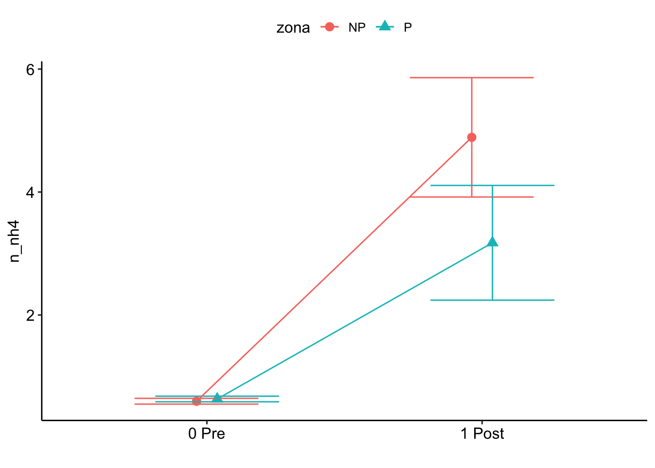

NO3

Check distribution

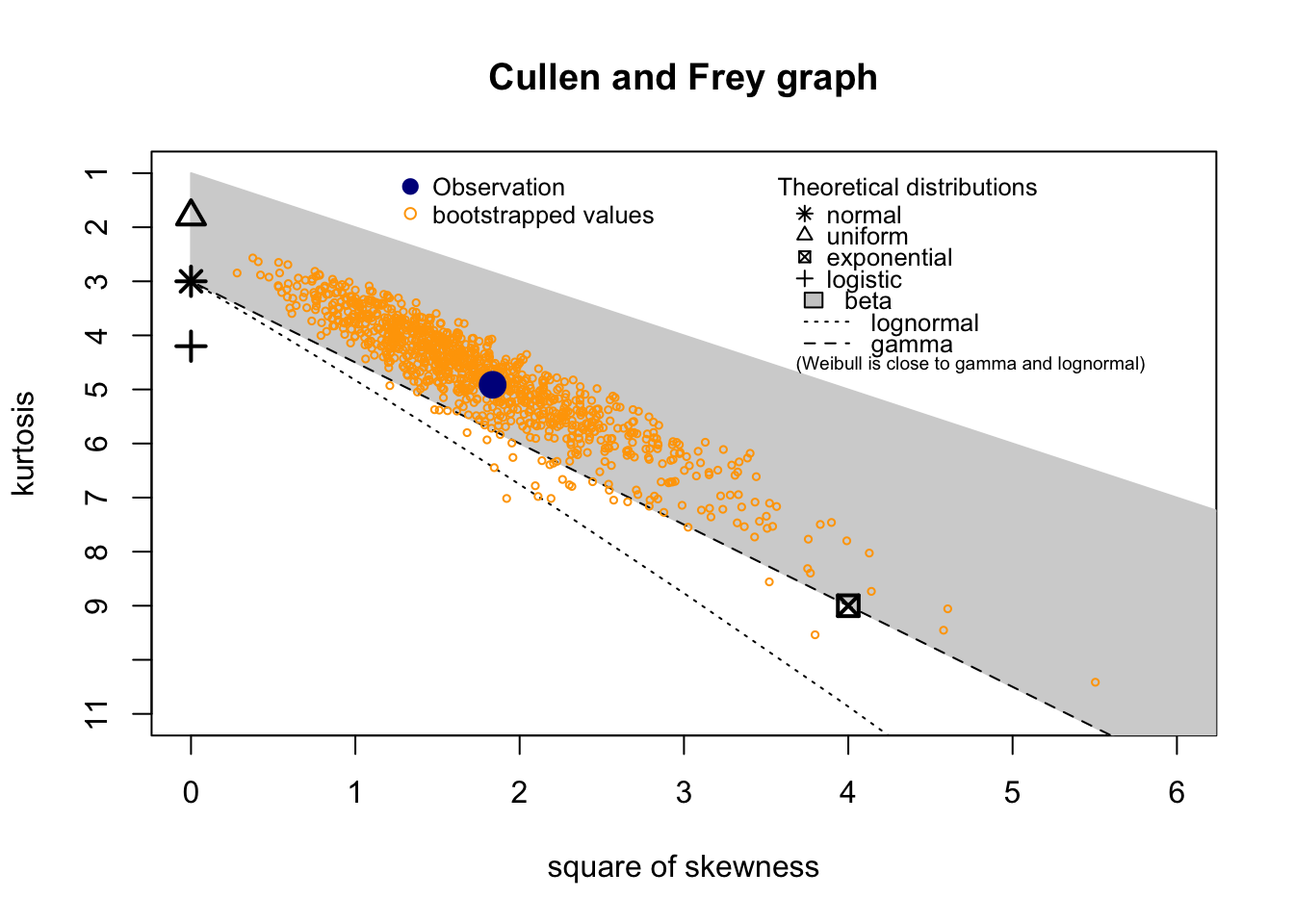
summary statistics
------
min:  0.197   max:  2.657 
median:  0.787 
mean:  0.8658526 
estimated sd:  0.4865887 
estimated skewness:  1.354862 
estimated kurtosis:  4.914124

Normality & Homocedasticity

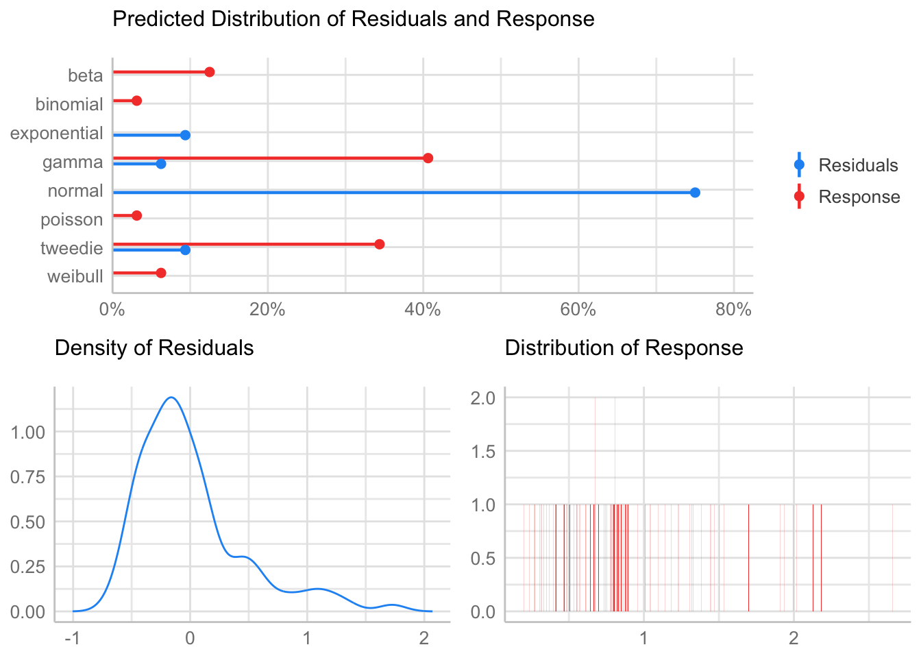
[1] "Variances homogeneity?"

OK: Variances in each of the groups are the same (Bartlett Test, p = 0.066).

[1] "Normality?"

Warning: Non-normality of residuals detected (p < .001).

Model

Gamma

Fitting one lmer() model. [DONE]
Calculating p-values. [DONE]

Mixed Model Anova Table (Type 3 tests, KR-method)

Model: n_no3 ~ pre_post_quema * zona + (1 | zona:geo_parcela_nombre)
Data: df_model
               Effect       df    F p.value
1      pre_post_quema 1, 85.07 1.02    .314
2                zona  1, 6.00 0.27    .620
3 pre_post_quema:zona 1, 85.07 0.28    .601
---
Signif. codes:  0 '***' 0.001 '**' 0.01 '*' 0.05 '+' 0.1 ' ' 1

Post-hoc

$`emmeans of pre_post_quema`
 pre_post_quema emmean    SE  df asymp.LCL asymp.UCL
 0 Pre            1.14 0.118 Inf     0.908      1.37
 1 Post           1.26 0.124 Inf     1.019      1.50

Results are averaged over the levels of: zona 
Results are given on the inverse (not the response) scale. 
Confidence level used: 0.95 

$`pairwise differences of pre_post_quema`
 1              estimate    SE  df z.ratio p.value
 0 Pre - 1 Post   -0.124 0.116 Inf -1.062  0.2884 

Results are averaged over the levels of: zona 
Note: contrasts are still on the inverse scale

$`emmeans of zona`
 zona emmean    SE  df asymp.LCL asymp.UCL
 NP     1.25 0.149 Inf     0.957      1.54
 P      1.15 0.145 Inf     0.867      1.44

Results are averaged over the levels of: pre_post_quema 
Results are given on the inverse (not the response) scale. 
Confidence level used: 0.95 

$`pairwise differences of zona`
 1      estimate    SE  df z.ratio p.value
 NP - P   0.0979 0.204 Inf 0.479   0.6318 

Results are averaged over the levels of: pre_post_quema 
Note: contrasts are still on the inverse scale

$`emmeans of pre_post_quema | zona`
zona = NP:
 pre_post_quema emmean    SE  df asymp.LCL asymp.UCL
 0 Pre            1.22 0.169 Inf     0.884      1.55
 1 Post           1.28 0.174 Inf     0.942      1.62

zona = P:
 pre_post_quema emmean    SE  df asymp.LCL asymp.UCL
 0 Pre            1.06 0.158 Inf     0.750      1.37
 1 Post           1.24 0.173 Inf     0.903      1.58

Results are given on the inverse (not the response) scale. 
Confidence level used: 0.95 

$`pairwise differences of pre_post_quema | zona`
zona = NP:
 2              estimate    SE  df z.ratio p.value
 0 Pre - 1 Post  -0.0671 0.169 Inf -0.397  0.6915 

zona = P:
 2              estimate    SE  df z.ratio p.value
 0 Pre - 1 Post  -0.1801 0.160 Inf -1.125  0.2605 

Note: contrasts are still on the inverse scale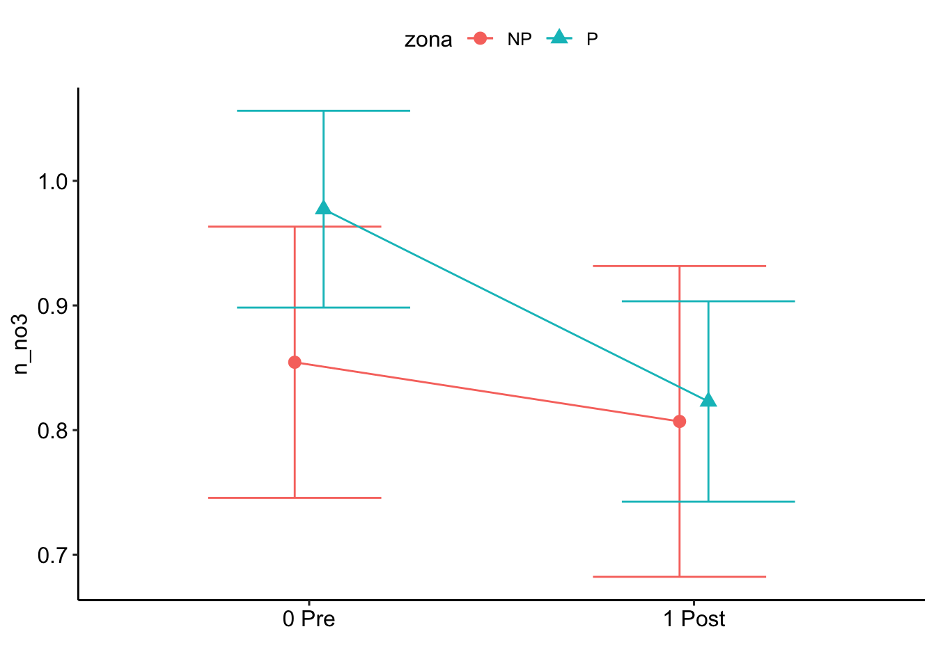

Resumen general

R version 4.0.2 (2020-06-22)
Platform: x86_64-apple-darwin17.0 (64-bit)
Running under: macOS Catalina 10.15.3

Matrix products: default
BLAS:   /Library/Frameworks/R.framework/Versions/4.0/Resources/lib/libRblas.dylib
LAPACK: /Library/Frameworks/R.framework/Versions/4.0/Resources/lib/libRlapack.dylib

locale:
[1] en_US.UTF-8/en_US.UTF-8/en_US.UTF-8/C/en_US.UTF-8/en_US.UTF-8

attached base packages:
[1] stats     graphics  grDevices utils     datasets  methods   base     

other attached packages:
 [1] glmmTMB_1.0.2.1    afex_0.28-1        performance_0.7.2  multcomp_1.4-16   
 [5] TH.data_1.0-10     mvtnorm_1.1-1      emmeans_1.5.4      lmerTest_3.1-3    
 [9] lme4_1.1-27.1      Matrix_1.3-2       fitdistrplus_1.1-3 survival_3.2-7    
[13] MASS_7.3-53        ggpubr_0.4.0       janitor_2.1.0      here_1.0.1        
[17] forcats_0.5.1      stringr_1.4.0      dplyr_1.0.6        purrr_0.3.4       
[21] readr_1.4.0        tidyr_1.1.3        tibble_3.1.2       ggplot2_3.3.5     
[25] tidyverse_1.3.1    rmdformats_1.0.1   knitr_1.31         workflowr_1.6.2   

loaded via a namespace (and not attached):
  [1] minqa_1.2.4         colorspace_2.0-0    glmmADMB_0.8.3.3   
  [4] ggsignif_0.6.0      ggridges_0.5.3      ellipsis_0.3.2     
  [7] rio_0.5.16          rprojroot_2.0.2     estimability_1.3   
 [10] snakecase_0.11.0    parameters_0.14.0   fs_1.5.0           
 [13] rstudioapi_0.13     farver_2.0.3        fansi_0.4.2        
 [16] lubridate_1.7.10    xml2_1.3.2          codetools_0.2-18   
 [19] splines_4.0.2       jsonlite_1.7.2      nloptr_1.2.2.2     
 [22] pbkrtest_0.5-0.1    broom_0.7.9         dbplyr_2.1.1       
 [25] effectsize_0.4.5    compiler_4.0.2      httr_1.4.2         
 [28] backports_1.2.1     assertthat_0.2.1    fastmap_1.1.0      
 [31] cli_2.5.0           formatR_1.8         later_1.1.0.1      
 [34] htmltools_0.5.2     tools_4.0.2         coda_0.19-4        
 [37] gtable_0.3.0        glue_1.4.2          reshape2_1.4.4     
 [40] Rcpp_1.0.7          carData_3.0-4       cellranger_1.1.0   
 [43] jquerylib_0.1.3     vctrs_0.3.8         nlme_3.1-152       
 [46] insight_0.14.4      xfun_0.23           openxlsx_4.2.3     
 [49] rvest_1.0.0         lifecycle_1.0.0     rstatix_0.6.0      
 [52] zoo_1.8-8           scales_1.1.1        hms_1.0.0          
 [55] promises_1.2.0.1    parallel_4.0.2      sandwich_3.0-0     
 [58] TMB_1.7.19          yaml_2.2.1          curl_4.3           
 [61] gridExtra_2.3       see_0.6.4           sass_0.3.1         
 [64] stringi_1.7.4       bayestestR_0.9.0    highr_0.8          
 [67] plotrix_3.8-1       randomForest_4.6-14 boot_1.3-26        
 [70] zip_2.1.1           R2admb_0.7.16.2     rlang_0.4.10       
 [73] pkgconfig_2.0.3     evaluate_0.14       lattice_0.20-41    
 [76] labeling_0.4.2      tidyselect_1.1.1    plyr_1.8.6         
 [79] magrittr_2.0.1      bookdown_0.21.6     R6_2.5.0           
 [82] generics_0.1.0      DBI_1.1.1           pillar_1.6.1       
 [85] haven_2.3.1         whisker_0.4         foreign_0.8-81     
 [88] withr_2.4.1         abind_1.4-5         modelr_0.1.8       
 [91] crayon_1.4.1        car_3.0-10          utf8_1.1.4         
 [94] rmarkdown_2.8       grid_4.0.2          readxl_1.3.1       
 [97] data.table_1.14.0   git2r_0.28.0        reprex_2.0.0       
[100] digest_0.6.27      
 [ reached getOption("max.print") -- omitted 5 entries ]

Pre- and post-fire anaylisis of soils

Prepare data

Modellize

Humedad

Check distribution

Normality & Homocedasticity

Model

Post-hoc

CIC

Check distribution

Normality & Homocedasticity

Model

Post-hoc

% C

Check distribution

Normality & Homocedasticity

Model

Post-hoc

% Fe

Check distribution

Normality & Homocedasticity

Model

Post-hoc

% K

Check distribution

Normality & Homocedasticity

Model

Post-hoc

% Mg

Check distribution

Normality & Homocedasticity

Model

Post-hoc

C/N

Check distribution

Normality & Homocedasticity

Model

Post-hoc

P

Check distribution

Normality & Homocedasticity

Model

Post-hoc

MO

Check distribution

Normality & Homocedasticity

Model

Post-hoc

% N

Check distribution

Normality & Homocedasticity

Model

Post-hoc

% Na

Check distribution

Normality & Homocedasticity

Model

Post-hoc

NH4

Check distribution

Normality & Homocedasticity

Model

Post-hoc

NO3

Check distribution

Normality & Homocedasticity

Model

Post-hoc

Resumen general