Genetic relationship matrix
Siming Zhao
2024-01-21
Last updated: 2024-01-23
Checks: 6 1
Knit directory: QBS-statsgen/
This reproducible R Markdown analysis was created with workflowr (version 1.6.2). The Checks tab describes the reproducibility checks that were applied when the results were created. The Past versions tab lists the development history.
The R Markdown is untracked by Git. To know which version of the R
Markdown file created these results, you’ll want to first commit it to
the Git repo. If you’re still working on the analysis, you can ignore
this warning. When you’re finished, you can run
wflow_publish to commit the R Markdown file and build the
HTML.
Great job! The global environment was empty. Objects defined in the global environment can affect the analysis in your R Markdown file in unknown ways. For reproduciblity it’s best to always run the code in an empty environment.
The command set.seed(20231230) was run prior to running
the code in the R Markdown file. Setting a seed ensures that any results
that rely on randomness, e.g. subsampling or permutations, are
reproducible.
Great job! Recording the operating system, R version, and package versions is critical for reproducibility.
Nice! There were no cached chunks for this analysis, so you can be confident that you successfully produced the results during this run.
Great job! Using relative paths to the files within your workflowr project makes it easier to run your code on other machines.
Great! You are using Git for version control. Tracking code development and connecting the code version to the results is critical for reproducibility.
The results in this page were generated with repository version 85e59dd. See the Past versions tab to see a history of the changes made to the R Markdown and HTML files.
Note that you need to be careful to ensure that all relevant files for
the analysis have been committed to Git prior to generating the results
(you can use wflow_publish or
wflow_git_commit). workflowr only checks the R Markdown
file, but you know if there are other scripts or data files that it
depends on. Below is the status of the Git repository when the results
were generated:
Ignored files:
    Ignored:    .Rproj.user/B81CBE6F/bibliography-index/
    Ignored:    .Rproj.user/B81CBE6F/ctx/
    Ignored:    .Rproj.user/B81CBE6F/pcs/
    Ignored:    .Rproj.user/B81CBE6F/presentation/
    Ignored:    .Rproj.user/B81CBE6F/profiles-cache/
    Ignored:    .Rproj.user/B81CBE6F/sources/per/
    Ignored:    .Rproj.user/B81CBE6F/tutorial/
    Ignored:    .Rproj.user/shared/notebooks/1C2AC29C-e1-gwas-power/
    Ignored:    .Rproj.user/shared/notebooks/1EB0B2DC-e1-gwas/1/s/ce0r78nx8keuu/
    Ignored:    .Rproj.user/shared/notebooks/1EB0B2DC-e1-gwas/1/s/csetup_chunk/
    Ignored:    .Rproj.user/shared/notebooks/1EB0B2DC-e1-gwas/1/s/czxn6jf8lsykc/
    Ignored:    .Rproj.user/shared/notebooks/26ED8139-e2-prs/
    Ignored:    .Rproj.user/shared/notebooks/BC66D613-e2-lmm/
    Ignored:    .Rproj.user/shared/notebooks/FCFC3BD0-e2-finemapping/
    Ignored:    data/e2-ori/
    Ignored:    data/e2/
    Ignored:    output/

Untracked files:
    Untracked:  analysis/e2-finemapping.Rmd
    Untracked:  analysis/e2-lmm.Rmd
    Untracked:  analysis/e2-prs.Rmd
    Untracked:  code/Bayesian-linear-regression.R

Unstaged changes:
    Modified:   .Rproj.user/B81CBE6F/persistent-state
    Modified:   .Rproj.user/B81CBE6F/sources/prop/4C8B7780
    Modified:   .Rproj.user/B81CBE6F/sources/prop/BBFFB970
    Modified:   .Rproj.user/B81CBE6F/sources/prop/INDEX
    Modified:   .Rproj.user/B81CBE6F/sources/s-e0e7218a/34A40D3B
    Modified:   .Rproj.user/B81CBE6F/sources/s-e0e7218a/34A40D3B-contents
    Deleted:    .Rproj.user/B81CBE6F/sources/s-e0e7218a/6C1FFABC
    Modified:   .Rproj.user/B81CBE6F/sources/s-e0e7218a/lock_file
    Modified:   .Rproj.user/shared/notebooks/paths
    Modified:   analysis/index.Rmd
    Deleted:    temp.csv
Note that any generated files, e.g. HTML, png, CSS, etc., are not included in this status report because it is ok for generated content to have uncommitted changes.
There are no past versions. Publish this analysis with
wflow_publish() to start tracking its development.
Before the class
- Download data
Download from here: https://rcweb.dartmouth.edu/Szhao/QBS148-statsgen/e2/.
- Plink
We have used plink in our first exercise class.
- R packages
Install ggplot2, data.table,
tidyverse if you don’t have them.
Data used in this analysis
- Genotype data The genotype data is given plink1 format:
oz.fam,oz.bim,oz.bed
Pay attention to the .fam file
head data/e2/oz.fam1400 1400t1 0 0 1 -9
1400 1400t2 0 0 2 -9
570 570t1 0 0 1 -9
570 570t2 0 0 1 -9
3413 3413t1 0 0 2 -9
3413 3413t2 0 0 1 -9
1911 1911t1 0 0 2 -9
1911 1911t2 0 0 2 -9
1403 1403t1 0 0 2 -9
1403 1403t2 0 0 1 -9The .fam file has 6 columns: Family ID, Individual ID, Fathers ID (0=missing), Mothers ID (0=missing), Sex (1=M, 2=F), Phenotype (-9=missing).
Now we can see there are related individuals in this cohort.
Get and plot GRM
Use plink to get GRM
plink --bfile data/e2/oz --make-grm-gz --out output/ozThis will generate ozbim.grm.gz and
ozbim.grm.id files in the output folder. Note:
you will need to create the output folder first if you
don’t have one.
To visualize this:
library("tidyverse")── Attaching packages ─────────────────────────────────────── tidyverse 1.3.1 ──✔ ggplot2 3.3.5 ✔ purrr 0.3.4
✔ tibble 3.1.2 ✔ dplyr 1.0.7
✔ tidyr 1.1.3 ✔ stringr 1.4.0
✔ readr 1.4.0 ✔ forcats 0.5.1── Conflicts ────────────────────────────────────────── tidyverse_conflicts() ──
✖ dplyr::filter() masks stats::filter()
✖ dplyr::lag() masks stats::lag()# these are plot functions:
tileplot <- function(mat)
{
mat = data.frame(mat)
mat$Var1 = factor(rownames(mat), levels=rownames(mat)) ## preserve rowname order
melted_mat <- gather(mat,key=Var2,value=value,-Var1)
melted_mat$Var2 = factor(melted_mat$Var2, levels=colnames(mat)) ## preserve colname order
rango = range(melted_mat$value)
pp <- ggplot(melted_mat,aes(x=Var1,y=Var2,fill=value)) + geom_tile() ##+scale_fill_gradientn(colours = c("#C00000", "#FF0000", "#FF8080", "#FFC0C0", "#FFFFFF", "#C0C0FF", "#8080FF", "#0000FF", "#0000C0"), limit = c(-1,1))
pp
}
grmgz2mat = function(grmhead)
{
## given plink like header, it reads thd grm file and returns matrix of grm
grm = read.table(paste0(grmhead,".grm.gz"),header=F)
grmid = read.table(paste0(grmhead,".grm.id"),header=F)
grmat = matrix(0,max(grm$V1),max(grm$V2))
rownames(grmat) = grmid$V2
colnames(grmat) = grmid$V2
## fill lower matrix of GRM
grmat[upper.tri(grmat,diag=TRUE)]= grm$V4
## make upper = lower, need to subtract diag
grmat + t(grmat) - diag(diag(grmat))
}## read grm calculated in plink into R matrix
grmat = grmgz2mat("output/oz")We can look at the distribution of diagonal values (ie the covariation of a person with themselves) using the following code. Usually we would expect the values to be close to 1. This teaching example only includes ~10,000 snps so there is more variation here than we would usually expect.
hist(diag(grmat), breaks=100)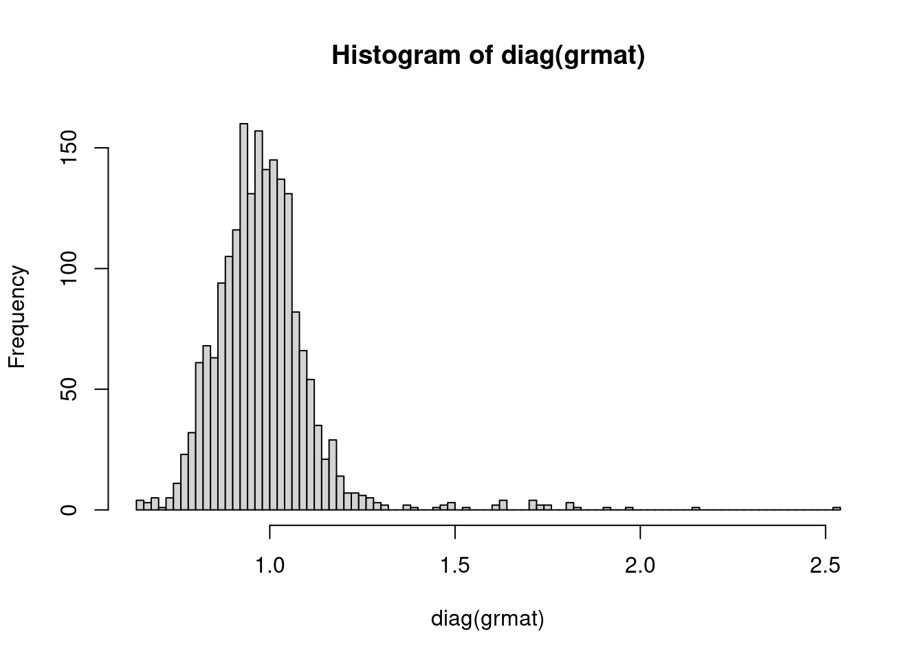
For off diagnal values, plot distribution. The off-diagonal elements of the GRM are two times the kinship coefficient. Related samples are inferred based on the range of estimated kinship coefficients = : >0.354, 0.354-0.177, 0.177-0.0884, and 0.0884-0.0442 that corresponds to duplicate/MZ twin, 1st-degree, 2nd-degree, and 3rd-degree relationships, respectively.
Plot distribution of kinship coefficient:
grmat.off <- c(grmat[upper.tri(grmat)])
hist(grmat.off[which(grmat.off>0.05)]/2, breaks=100, xlim=c(0.05,0.3))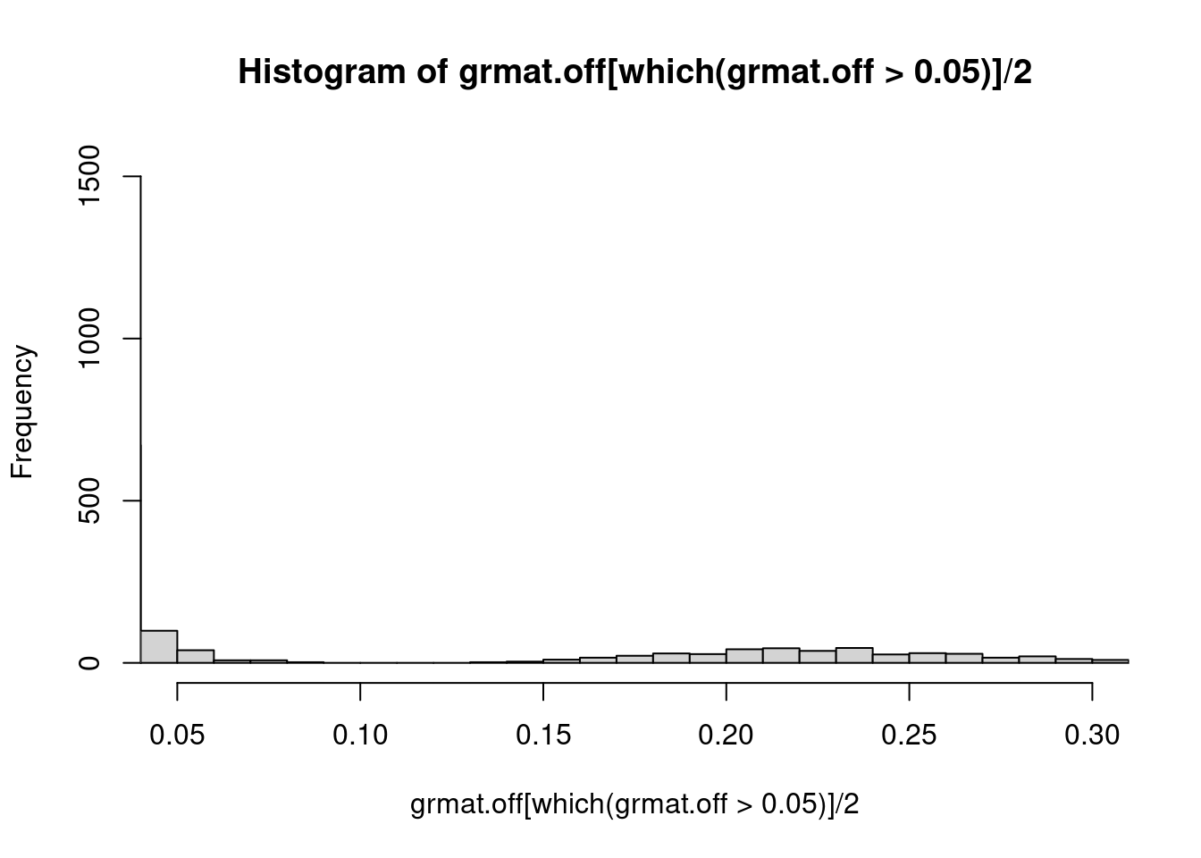 Plot GRM for a few families:
fam = read.table("data/e2/oz.fam") # second column is IID (individual ID)
head(fam, n= 6)
V1 V2 V3 V4 V5 V6
1 1400 1400t1 0 0 1 -9
2 1400 1400t2 0 0 2 -9
3 570 570t1 0 0 1 -9
4 570 570t2 0 0 1 -9
5 3413 3413t1 0 0 2 -9
6 3413 3413t2 0 0 1 -9ind = fam[1:6,2]
print(ind)[1] "1400t1" "1400t2" "570t1" "570t2" "3413t1" "3413t2"There are three families: 1400, 570, and 3413. Each family has two individuals.
tileplot(grmat[ind,ind]/2)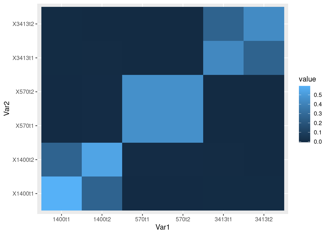
–> –>
Credits
GRM visualization from Haky Im: https://hakyimlab.github.io/hgen471/L8-GRM.html Data from https://www.colorado.edu/ibg/international-workshop/2022-international-statistical-genetics-workshop/syllabus/polygenic-scores
sessionInfo()R version 4.1.0 (2021-05-18)
Platform: x86_64-pc-linux-gnu (64-bit)
Running under: CentOS Linux 7 (Core)
Matrix products: default
BLAS: /software/R-4.1.0-no-openblas-el7-x86_64/lib64/R/lib/libRblas.so
LAPACK: /software/R-4.1.0-no-openblas-el7-x86_64/lib64/R/lib/libRlapack.so
locale:
[1] LC_CTYPE=en_US.UTF-8 LC_NUMERIC=C LC_TIME=C
[4] LC_COLLATE=C LC_MONETARY=C LC_MESSAGES=C
[7] LC_PAPER=C LC_NAME=C LC_ADDRESS=C
[10] LC_TELEPHONE=C LC_MEASUREMENT=C LC_IDENTIFICATION=C
attached base packages:
[1] stats graphics grDevices utils datasets methods base
other attached packages:
[1] forcats_0.5.1 stringr_1.4.0 dplyr_1.0.7 purrr_0.3.4
[5] readr_1.4.0 tidyr_1.1.3 tibble_3.1.2 ggplot2_3.3.5
[9] tidyverse_1.3.1
loaded via a namespace (and not attached):
[1] Rcpp_1.0.9 lubridate_1.7.10 assertthat_0.2.1 rprojroot_2.0.2
[5] digest_0.6.27 utf8_1.2.1 R6_2.5.0 cellranger_1.1.0
[9] backports_1.2.1 reprex_2.0.0 evaluate_0.20 highr_0.9
[13] httr_1.4.2 pillar_1.6.1 rlang_1.1.0 readxl_1.3.1
[17] rstudioapi_0.13 jquerylib_0.1.4 rmarkdown_2.21 labeling_0.4.2
[21] munsell_0.5.0 broom_0.7.8 compiler_4.1.0 httpuv_1.6.1
[25] modelr_0.1.8 xfun_0.38 pkgconfig_2.0.3 htmltools_0.5.5
[29] tidyselect_1.1.1 workflowr_1.6.2 fansi_0.5.0 crayon_1.5.2
[33] dbplyr_2.1.1 withr_2.5.0 later_1.2.0 grid_4.1.0
[37] jsonlite_1.7.2 gtable_0.3.0 lifecycle_1.0.3 DBI_1.1.1
[41] git2r_0.28.0 magrittr_2.0.1 scales_1.1.1 cli_3.6.1
[45] stringi_1.6.2 cachem_1.0.5 farver_2.1.0 fs_1.6.1
[49] promises_1.2.0.1 xml2_1.3.2 bslib_0.4.2 ellipsis_0.3.2
[53] generics_0.1.0 vctrs_0.3.8 tools_4.1.0 glue_1.4.2
[57] hms_1.1.0 fastmap_1.1.0 yaml_2.2.1 colorspace_2.0-2
[61] rvest_1.0.0 knitr_1.42 haven_2.4.1 sass_0.4.0