Seven Correlated Tissues Simulation
shengqian
2023-12-30
Last updated: 2024-01-16
Checks: 6 1
Knit directory: multigroup_ctwas_analysis/
This reproducible R Markdown analysis was created with workflowr (version 1.7.0). The Checks tab describes the reproducibility checks that were applied when the results were created. The Past versions tab lists the development history.
The R Markdown file has unstaged changes. To know which version of the R Markdown file created these results, you’ll want to first commit it to the Git repo. If you’re still working on the analysis, you can ignore this warning. When you’re finished, you can run wflow_publish to commit the R Markdown file and build the HTML.
Great job! The global environment was empty. Objects defined in the global environment can affect the analysis in your R Markdown file in unknown ways. For reproduciblity it’s best to always run the code in an empty environment.
The command set.seed(20231112) was run prior to running the code in the R Markdown file. Setting a seed ensures that any results that rely on randomness, e.g. subsampling or permutations, are reproducible.
Great job! Recording the operating system, R version, and package versions is critical for reproducibility.
Nice! There were no cached chunks for this analysis, so you can be confident that you successfully produced the results during this run.
Great job! Using relative paths to the files within your workflowr project makes it easier to run your code on other machines.
Great! You are using Git for version control. Tracking code development and connecting the code version to the results is critical for reproducibility.
The results in this page were generated with repository version a644230. See the Past versions tab to see a history of the changes made to the R Markdown and HTML files.
Note that you need to be careful to ensure that all relevant files for the analysis have been committed to Git prior to generating the results (you can use wflow_publish or wflow_git_commit). workflowr only checks the R Markdown file, but you know if there are other scripts or data files that it depends on. Below is the status of the Git repository when the results were generated:
Untracked files:
    Untracked:  analysis/simulation_E_S_three_tissues.Rmd

Unstaged changes:
    Modified:   analysis/simulation_seven_tissues_correlated.Rmd
Note that any generated files, e.g. HTML, png, CSS, etc., are not included in this status report because it is ok for generated content to have uncommitted changes.
These are the previous versions of the repository in which changes were made to the R Markdown (analysis/simulation_seven_tissues_correlated.Rmd) and HTML (docs/simulation_seven_tissues_correlated.html) files. If you’ve configured a remote Git repository (see ?wflow_git_remote), click on the hyperlinks in the table below to view the files as they were in that past version.
| File | Version | Author | Date | Message |
|---|---|---|---|---|
| Rmd | a644230 | sq-96 | 2024-01-15 | update |
| html | a644230 | sq-96 | 2024-01-15 | update |
| Rmd | 932e682 | sq-96 | 2024-01-15 | update |
| html | 932e682 | sq-96 | 2024-01-15 | update |
| Rmd | 4d024a0 | sq-96 | 2024-01-03 | update |
| html | 4d024a0 | sq-96 | 2024-01-03 | update |
| Rmd | 690e29e | sq-96 | 2024-01-03 | update |
| html | 690e29e | sq-96 | 2024-01-03 | update |
| Rmd | 2f6c0dd | sq-96 | 2023-12-30 | update |
| html | 2f6c0dd | sq-96 | 2023-12-30 | update |
| Rmd | 0a32579 | sq-96 | 2023-12-30 | update |
| html | 0a32579 | sq-96 | 2023-12-30 | update |
A simulation of seven correlated tissues is conducted to evaluate cTWAS performance (parameter estimation, PIP calibration …). Seven tissues used in this simulation are Artery Aorta, Spleen, Skin (not sun exposed suprapubic), Lung, Adipose Subcutaneous, Pancreas, Heart Artial Appendage. Pairwise correlation of gene expression are with 0.6-0.8. The first three tissues are set to be causal and the other four tissues are non-causal.
                                Adipose_Subcutaneous      Lung Artery_Aorta
Adipose_Subcutaneous                               1 0.8001729    0.7837312
Lung                                              NA 1.0000000    0.7378609
Artery_Aorta                                      NA        NA    1.0000000
Heart_Atrial_Appendage                            NA        NA           NA
Skin_Not_Sun_Exposed_Suprapubic                   NA        NA           NA
Spleen                                            NA        NA           NA
Pancreas                                          NA        NA           NA
                                Heart_Atrial_Appendage
Adipose_Subcutaneous                         0.7330170
Lung                                         0.7144555
Artery_Aorta                                 0.7395328
Heart_Atrial_Appendage                       1.0000000
Skin_Not_Sun_Exposed_Suprapubic                     NA
Spleen                                              NA
Pancreas                                            NA
                                Skin_Not_Sun_Exposed_Suprapubic    Spleen
Adipose_Subcutaneous                                  0.6954358 0.7152079
Lung                                                  0.6977584 0.7773205
Artery_Aorta                                          0.6357966 0.6740020
Heart_Atrial_Appendage                                0.6180385 0.6302362
Skin_Not_Sun_Exposed_Suprapubic                       1.0000000 0.6336601
Spleen                                                       NA 1.0000000
Pancreas                                                     NA        NA
                                 Pancreas
Adipose_Subcutaneous            0.6917465
Lung                            0.6969056
Artery_Aorta                    0.6758016
Heart_Atrial_Appendage          0.6620150
Skin_Not_Sun_Exposed_Suprapubic 0.6635378
Spleen                          0.6907535
Pancreas                        1.0000000
It current has two settings:
- 3% PVE, 0.9% \(\pi\) for causal tissues, 0.5% PVE, 0.15% \(\pi\) for non-causal tissues and 30% PVE, 2.5e-4 \(\pi\) for SNP.
- 3% PVE, 0.9% \(\pi\) for causal tissues, 0% PVE, 0% \(\pi\) for non-causal tissues and 30% PVE, 2.5e-4 \(\pi\) for SNP.
We observed that cTWAS always tend to overestimate PVE of non-causal tissues because parameters won’t be shrunk exactly to 0. Therefore, we assign non-zero (but very low) PVE to non-causal tissues in the first setting to check if it helps simulation results.
Simulation 1: 3% PVE for Causal Tissues and 0.5% PVE for Non-causal Tissues.
Results using Combined PIP Threshold
simutag n_causal_combined n_detected_comb_pip n_detected_comb_pip_in_causal
1 1-1 312 78 70
2 1-2 345 88 77
3 1-3 323 60 58
4 1-4 320 59 56
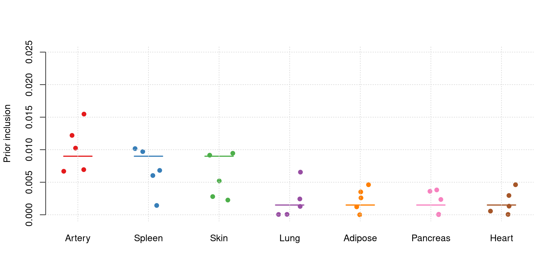
5 1-5 302 55 51[1] 0.9176471Estimated Prior Inclusion Probability
Estimated PVE
Separate effect size parameters
For the cTWAS analysis, each tissue had its own prior inclusion parameter and effect size parameter.
Results using Combined PIP Threshold
  simutag n_causal_combined n_detected_comb_pip n_detected_comb_pip_in_causal
1     1-1               312                  76                            68
2     1-2               345                  88                            76
3     1-3               323                  62                            59
4     1-4               320                  56                            53
5     1-5               302                  54                            50
[1] 0.9107143Estimated Prior Inclusion Probability
y1 <- results_df$prior_mashr_Artery_Aorta
y2 <- results_df$prior_mashr_Spleen
y3 <- results_df$prior_mashr_Skin_Not_Sun_Exposed_Suprapubic
y4 <- results_df$prior_mashr_Lung
y5 <- results_df$prior_mashr_Adipose_Subcutaneous
y6 <- results_df$prior_mashr_Pancreas
y7 <- results_df$prior_mashr_Heart_Atrial_Appendage

truth <- rbind(c(1,0.009),c(2,0.009),c(3,0.009),c(4,0.0015),c(5,0.0015),c(6,0.0015),c(7,0.0015))
est <- rbind(cbind(1,y1),cbind(2,y2),cbind(3,y3),cbind(4,y4),cbind(5,y5),cbind(6,y6),cbind(7,y7))
plot_par_7(truth,est,xlabels = c("Artery","Spleen","Skin","Lung","Adipose","Pancreas","Heart"),ylim=c(0,0.025),ylab="Prior inclusion")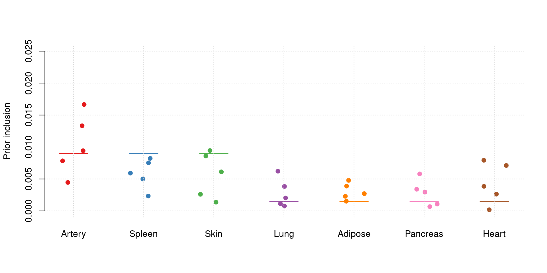
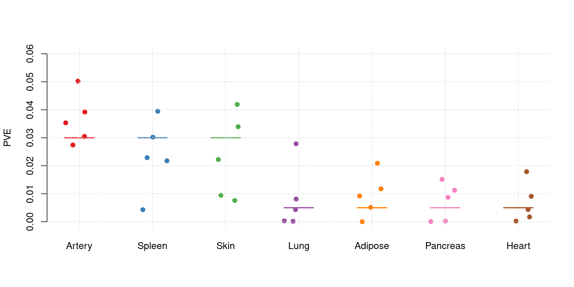
Estimated PVE
y1 <- results_df$pve_mashr_Artery_Aorta
y2 <- results_df$pve_mashr_Spleen
y3 <- results_df$pve_mashr_Skin_Not_Sun_Exposed_Suprapubic
y4 <- results_df$pve_mashr_Lung
y5 <- results_df$pve_mashr_Adipose_Subcutaneous
y6 <- results_df$pve_mashr_Pancreas
y7 <- results_df$pve_mashr_Heart_Atrial_Appendage

truth <- rbind(c(1,0.03),c(2,0.03),c(3,0.03),c(4,0.005),c(5,0.005),c(6,0.005),c(7,0.005))
est <- rbind(cbind(1,y1),cbind(2,y2),cbind(3,y3),cbind(4,y4),cbind(5,y5),cbind(6,y6),cbind(7,y7))
plot_par_7(truth,est,xlabels = c("Artery","Spleen","Skin","Lung","Adipose","Pancreas","Heart"),ylim=c(0,0.06),ylab="PVE")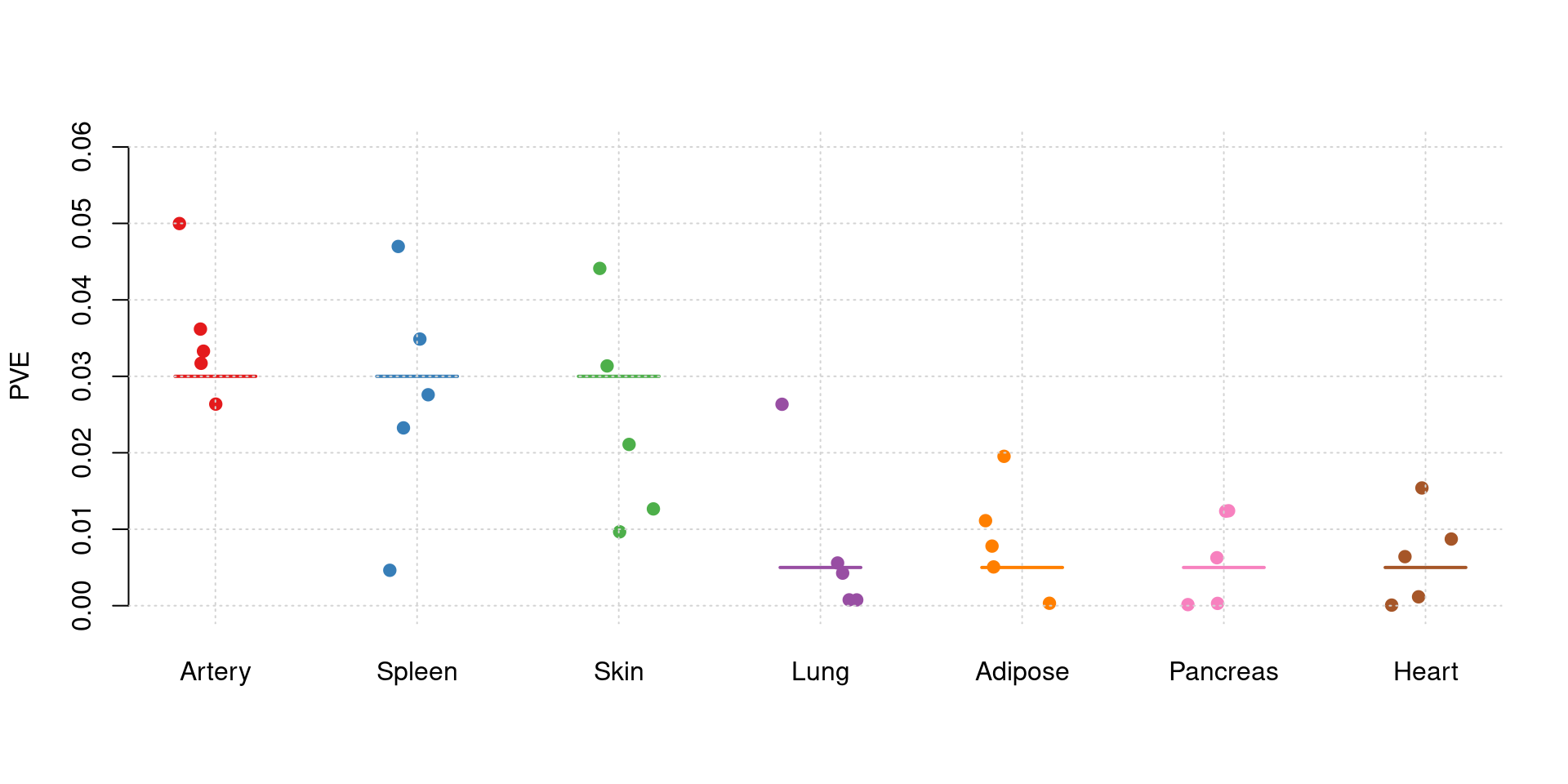
Simulation 2: 3% PVE for Causal Tissues and 0% PVE for Non-causal Tissues.
Results using Combined PIP Threshold
  simutag n_causal_combined n_detected_comb_pip n_detected_comb_pip_in_causal
1     2-1               250                  66                            58
2     2-2               274                  51                            44
3     2-3               261                  50                            44
4     2-4               246                  51                            39
5     2-5               255                  43                            40
[1] 0.862069Estimated Prior Inclusion Probability
y1 <- results_df$prior_mashr_Artery_Aorta
y2 <- results_df$prior_mashr_Spleen
y3 <- results_df$prior_mashr_Skin_Not_Sun_Exposed_Suprapubic
y4 <- results_df$prior_mashr_Lung
y5 <- results_df$prior_mashr_Adipose_Subcutaneous
y6 <- results_df$prior_mashr_Pancreas
y7 <- results_df$prior_mashr_Heart_Atrial_Appendage

truth <- rbind(c(1,0.009),c(2,0.009),c(3,0.009),c(4,0),c(5,0),c(6,0),c(7,0))
est <- rbind(cbind(1,y1),cbind(2,y2),cbind(3,y3),cbind(4,y4),cbind(5,y5),cbind(6,y6),cbind(7,y7))
plot_par_7(truth,est,xlabels = c("Artery","Spleen","Skin","Lung","Adipose","Pancreas","Heart"),ylim=c(0,0.025),ylab="Prior inclusion")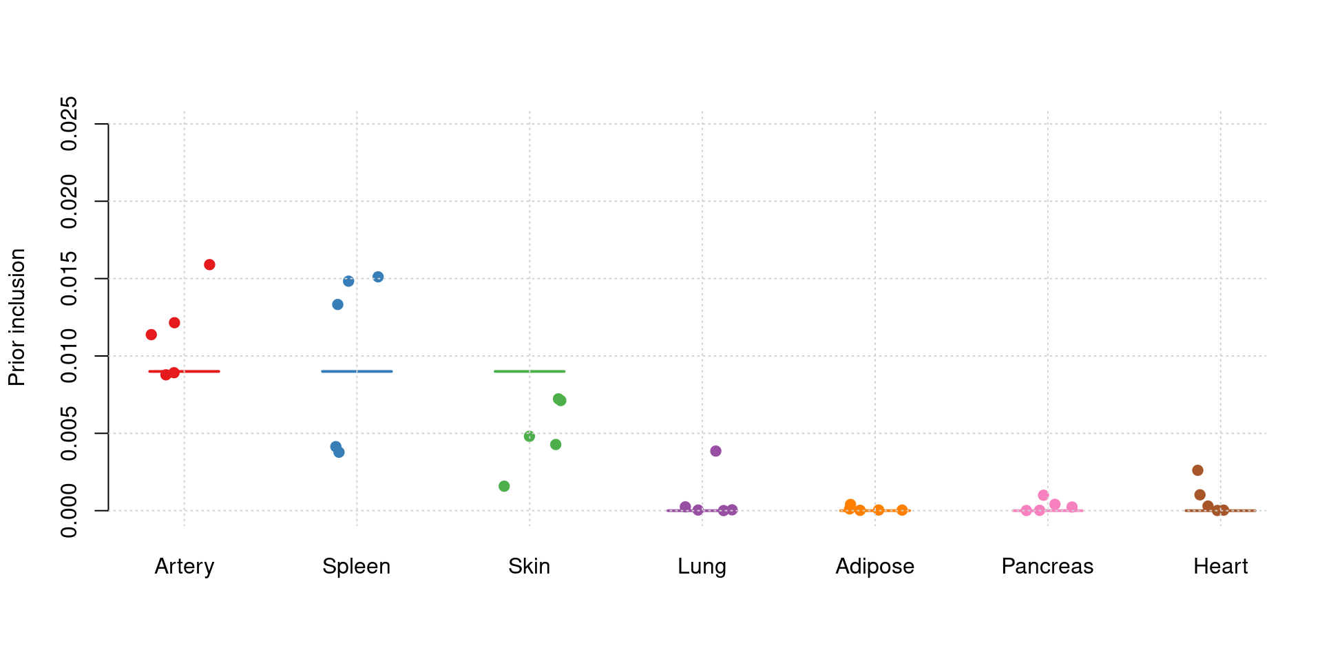
Estimated PVE
y1 <- results_df$pve_mashr_Artery_Aorta
y2 <- results_df$pve_mashr_Spleen
y3 <- results_df$pve_mashr_Skin_Not_Sun_Exposed_Suprapubic
y4 <- results_df$pve_mashr_Lung
y5 <- results_df$pve_mashr_Adipose_Subcutaneous
y6 <- results_df$pve_mashr_Pancreas
y7 <- results_df$pve_mashr_Heart_Atrial_Appendage

truth <- rbind(c(1,0.03),c(2,0.03),c(3,0.03),c(4,0),c(5,0),c(6,0),c(7,0))
est <- rbind(cbind(1,y1),cbind(2,y2),cbind(3,y3),cbind(4,y4),cbind(5,y5),cbind(6,y6),cbind(7,y7))
plot_par_7(truth,est,xlabels = c("Artery","Spleen","Skin","Lung","Adipose","Pancreas","Heart"),ylim=c(0,0.06),ylab="PVE")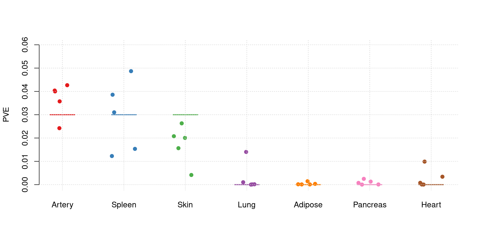
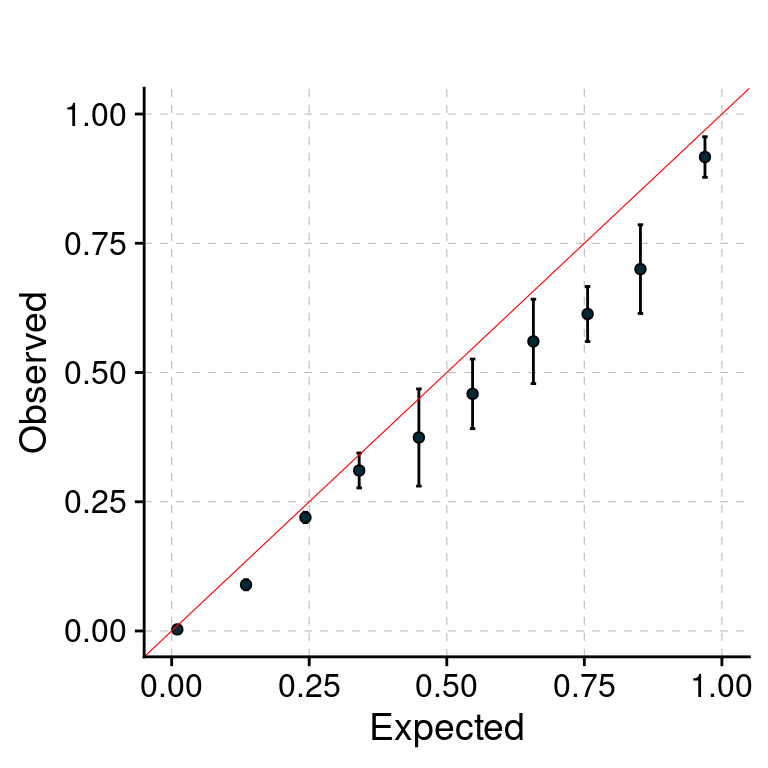
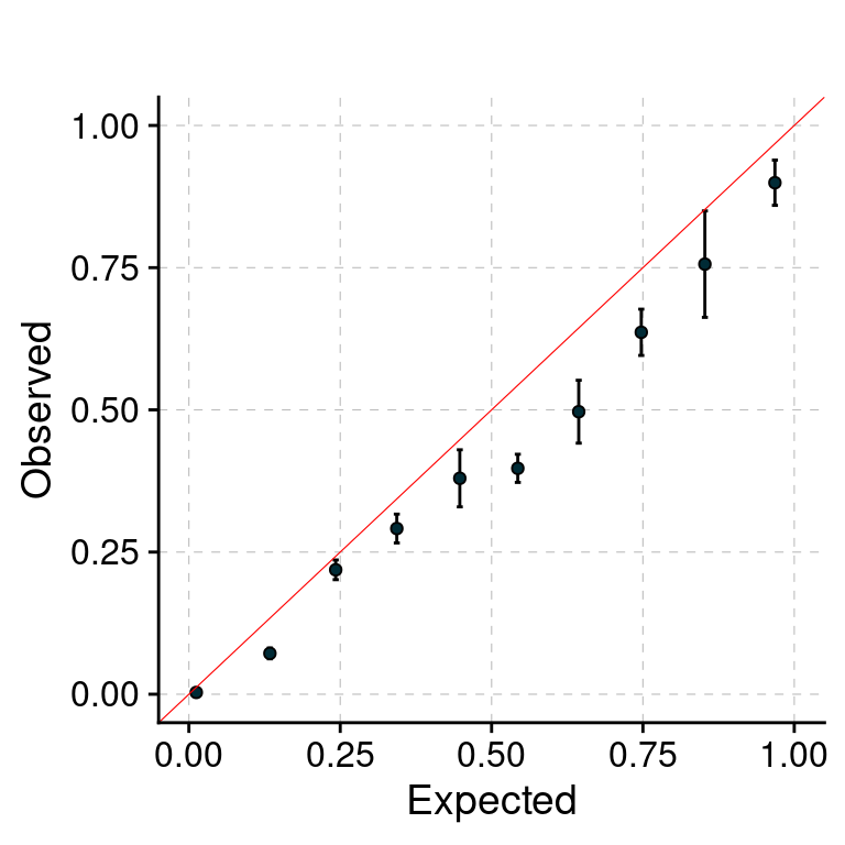
PIP Calibration Plot
f1 <- plot_PIP(configtag, runtag, paste(2, 1:5, sep = "-"), main = "")
f1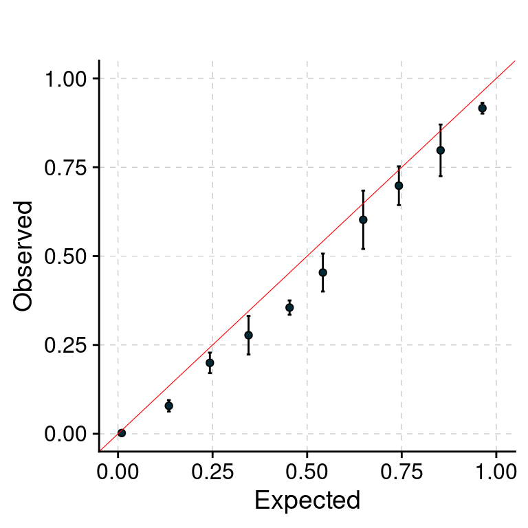
| Version | Author | Date |
|---|---|---|
| 932e682 | sq-96 | 2024-01-15 |
Separate effect size parameters
Results using Combined PIP Threshold
  simutag n_causal_combined n_detected_comb_pip n_detected_comb_pip_in_causal
1     2-1               250                  63                            56
2     2-2               274                  50                            43
3     2-3               261                  48                            41
4     2-4               246                  51                            39
5     2-5               255                  41                            39
[1] 0.8616601Estimated Prior Inclusion Probability
y1 <- results_df$prior_mashr_Artery_Aorta
y2 <- results_df$prior_mashr_Spleen
y3 <- results_df$prior_mashr_Skin_Not_Sun_Exposed_Suprapubic
y4 <- results_df$prior_mashr_Lung
y5 <- results_df$prior_mashr_Adipose_Subcutaneous
y6 <- results_df$prior_mashr_Pancreas
y7 <- results_df$prior_mashr_Heart_Atrial_Appendage


truth <- rbind(c(1,0.009),c(2,0.009),c(3,0.009),c(4,0),c(5,0),c(6,0),c(7,0))
est <- rbind(cbind(1,y1),cbind(2,y2),cbind(3,y3),cbind(4,y4),cbind(5,y5),cbind(6,y6),cbind(7,y7))
plot_par_7(truth,est,xlabels = c("Artery","Spleen","Skin","Lung","Adipose","Pancreas","Heart"),ylim=c(0,0.025),ylab="Prior inclusion")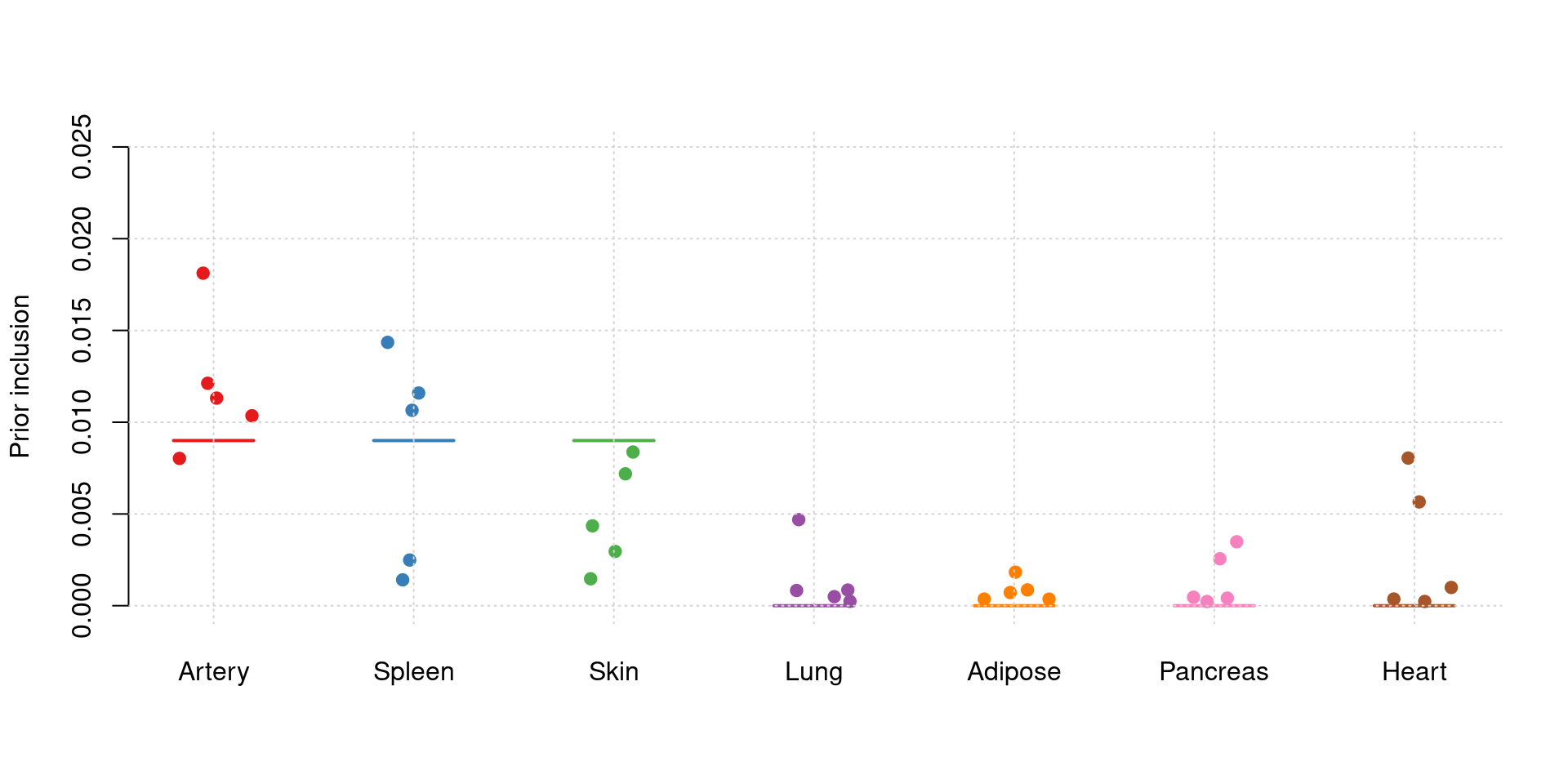
Estimated PVE
y1 <- results_df$pve_mashr_Artery_Aorta
y2 <- results_df$pve_mashr_Spleen
y3 <- results_df$pve_mashr_Skin_Not_Sun_Exposed_Suprapubic
y4 <- results_df$pve_mashr_Lung
y5 <- results_df$pve_mashr_Adipose_Subcutaneous
y6 <- results_df$pve_mashr_Pancreas
y7 <- results_df$pve_mashr_Heart_Atrial_Appendage

truth <- rbind(c(1,0.03),c(2,0.03),c(3,0.03),c(4,0),c(5,0),c(6,0),c(7,0))
est <- rbind(cbind(1,y1),cbind(2,y2),cbind(3,y3),cbind(4,y4),cbind(5,y5),cbind(6,y6),cbind(7,y7))
plot_par_7(truth,est,xlabels = c("Artery","Spleen","Skin","Lung","Adipose","Pancreas","Heart"),ylim=c(0,0.06),ylab="PVE")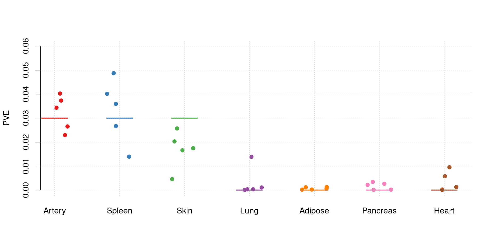
PIP Calibration Plot
f1 <- plot_PIP(configtag, runtag, paste(2, 1:5, sep = "-"), main = "")
f1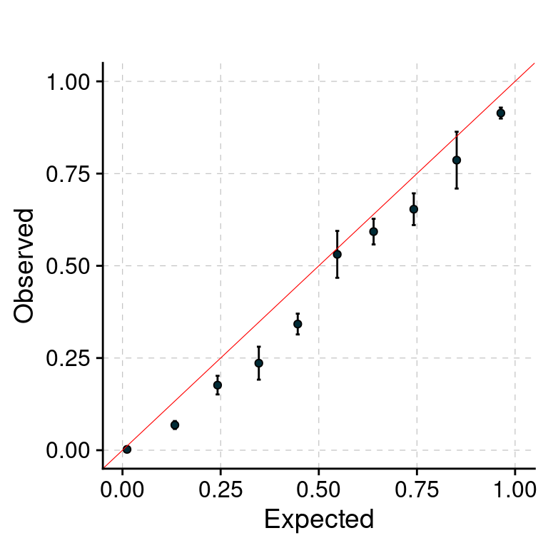
sessionInfo()R version 4.1.0 (2021-05-18)
Platform: x86_64-pc-linux-gnu (64-bit)
Running under: CentOS Linux 7 (Core)
Matrix products: default
BLAS/LAPACK: /software/openblas-0.3.13-el7-x86_64/lib/libopenblas_haswellp-r0.3.13.so
locale:
[1] LC_CTYPE=en_US.UTF-8 LC_NUMERIC=C
[3] LC_TIME=en_US.UTF-8 LC_COLLATE=en_US.UTF-8
[5] LC_MONETARY=en_US.UTF-8 LC_MESSAGES=en_US.UTF-8
[7] LC_PAPER=en_US.UTF-8 LC_NAME=C
[9] LC_ADDRESS=C LC_TELEPHONE=C
[11] LC_MEASUREMENT=en_US.UTF-8 LC_IDENTIFICATION=C
attached base packages:
[1] stats graphics grDevices utils datasets methods base
other attached packages:
[1] plyr_1.8.8 ggpubr_0.6.0 plotrix_3.8-4 cowplot_1.1.1
[5] ggplot2_3.4.0 data.table_1.14.6 ctwas_0.1.40 workflowr_1.7.0
loaded via a namespace (and not attached):
[1] Rcpp_1.0.9 lattice_0.20-44 tidyr_1.3.0 getPass_0.2-2
[5] ps_1.7.2 assertthat_0.2.1 rprojroot_2.0.3 digest_0.6.31
[9] foreach_1.5.2 utf8_1.2.2 R6_2.5.1 backports_1.2.1
[13] evaluate_0.19 highr_0.9 httr_1.4.4 pillar_1.8.1
[17] rlang_1.1.1 rstudioapi_0.14 car_3.1-1 whisker_0.4.1
[21] callr_3.7.3 jquerylib_0.1.4 Matrix_1.3-3 rmarkdown_2.19
[25] labeling_0.4.2 stringr_1.5.0 munsell_0.5.0 broom_1.0.2
[29] compiler_4.1.0 httpuv_1.6.7 xfun_0.35 pkgconfig_2.0.3
[33] htmltools_0.5.4 tidyselect_1.2.0 tibble_3.1.8 logging_0.10-108
[37] codetools_0.2-18 fansi_1.0.3 dplyr_1.0.10 withr_2.5.0
[41] later_1.3.0 grid_4.1.0 jsonlite_1.8.4 gtable_0.3.1
[45] lifecycle_1.0.3 DBI_1.1.3 git2r_0.30.1 magrittr_2.0.3
[49] scales_1.2.1 carData_3.0-4 cli_3.6.1 stringi_1.7.8
[53] cachem_1.0.6 farver_2.1.0 ggsignif_0.6.4 fs_1.5.2
[57] promises_1.2.0.1 pgenlibr_0.3.2 bslib_0.4.1 vctrs_0.6.3
[61] generics_0.1.3 iterators_1.0.14 tools_4.1.0 glue_1.6.2
[65] purrr_1.0.2 abind_1.4-5 processx_3.8.0 fastmap_1.1.0
[69] yaml_2.3.6 colorspace_2.0-3 rstatix_0.7.2 knitr_1.41
[73] sass_0.4.4