Simple example of how a p value translates to a Bayes Factor
Matthew Stephens
2016-04-20
Last updated: 2019-03-31
Checks: 6 0
Knit directory: fiveMinuteStats/analysis/
This reproducible R Markdown analysis was created with workflowr (version 1.2.0). The Report tab describes the reproducibility checks that were applied when the results were created. The Past versions tab lists the development history.
Great! Since the R Markdown file has been committed to the Git repository, you know the exact version of the code that produced these results.
Great job! The global environment was empty. Objects defined in the global environment can affect the analysis in your R Markdown file in unknown ways. For reproduciblity it’s best to always run the code in an empty environment.
The command set.seed(12345) was run prior to running the code in the R Markdown file. Setting a seed ensures that any results that rely on randomness, e.g. subsampling or permutations, are reproducible.
Great job! Recording the operating system, R version, and package versions is critical for reproducibility.
Nice! There were no cached chunks for this analysis, so you can be confident that you successfully produced the results during this run.
Great! You are using Git for version control. Tracking code development and connecting the code version to the results is critical for reproducibility. The version displayed above was the version of the Git repository at the time these results were generated.
Note that you need to be careful to ensure that all relevant files for the analysis have been committed to Git prior to generating the results (you can use wflow_publish or wflow_git_commit). workflowr only checks the R Markdown file, but you know if there are other scripts or data files that it depends on. Below is the status of the Git repository when the results were generated:
Ignored files:
    Ignored:    .Rhistory
    Ignored:    .Rproj.user/
    Ignored:    analysis/.Rhistory
    Ignored:    analysis/bernoulli_poisson_process_cache/

Untracked files:
    Untracked:  _workflowr.yml
    Untracked:  analysis/CI.Rmd
    Untracked:  analysis/gibbs_structure.Rmd
    Untracked:  analysis/libs/
    Untracked:  analysis/results.Rmd
    Untracked:  analysis/shiny/tester/
    Untracked:  docs/MH_intro_files/
    Untracked:  docs/citations.bib
    Untracked:  docs/hmm_files/
    Untracked:  docs/libs/
    Untracked:  docs/shiny/tester/
Note that any generated files, e.g. HTML, png, CSS, etc., are not included in this status report because it is ok for generated content to have uncommitted changes.
These are the previous versions of the R Markdown and HTML files. If you’ve configured a remote Git repository (see ?wflow_git_remote), click on the hyperlinks in the table below to view them.
| File | Version | Author | Date | Message |
|---|---|---|---|---|
| html | 34bcc51 | John Blischak | 2017-03-06 | Build site. |
| Rmd | 2aa70fe | John Blischak | 2017-03-06 | Manually udpate some Rmd files. |
| Rmd | 5fbc8b5 | John Blischak | 2017-03-06 | Update workflowr project with wflow_update (version 0.4.0). |
| Rmd | 391ba3c | John Blischak | 2017-03-06 | Remove front and end matter of non-standard templates. |
| html | fb0f6e3 | stephens999 | 2017-03-03 | Merge pull request #33 from mdavy86/f/review |
| Rmd | 51fc1e0 | Marcus Davy | 2017-02-27 | add Sellke et al citation |
| html | c3b365a | John Blischak | 2017-01-02 | Build site. |
| Rmd | 67a8575 | John Blischak | 2017-01-02 | Use external chunk to set knitr chunk options. |
| Rmd | 5ec12c7 | John Blischak | 2017-01-02 | Use session-info chunk. |
| Rmd | 47f75ca | stephens999 | 2016-04-20 | add BF and p value comparison |
Pre-requisites
You should know what a Bayes Factor is and what a p value is.
Overview
Sellke et al (Thomas Sellke 2001) study the following question (paraphrased and shortened here).
Consider the situation in which experimental drugs D1; D2; D3; etc are to be tested. Each test will be thought of as completely independent; we simply have a series of tests so that we can explore the frequentist properties of p values. In each test, the following hypotheses are to be tested: \[H_0 : D_i \text{ has negligible effect}\] versus \[H_1 : D_i \text{ has a non-negligible effect}.\]
Suppose that one of these tests results in a p value \(\approx p\). The question we consider is: How strong is the evidence that the drug in question has a non-negligible effect?
The answer to this question has to depend on the distribution of effects under \(H_1\). However, Sellke et al derive a bound for the Bayes Factor. Specifically they show that, provided \(p<1/e\), the BF in favor of \(H_1\) is not larger than \[1/B(p) = -[e p \log(p)]^{-1}.\] (Note: the inverse comes from the fact that here we consider the BF in favor of \(H_1\), whereas Sellke et al consider the BF in favor of H_0).
Here we illustrate this result using Bayes Theorem to do calculations under a simple scenario.
Details
Let \(\theta_i\) denote the effect of drug \(D_i\). We will translate the null \(H_0\) above to mean \(\theta_i=0\). We will also make an assumption that the effects of the non-null drugs are normally distributed \(N(0,\sigma^2)\), where the value of \(\sigma\) determines how different the typical effect is from 0.
Thus we have: \[H_{0i}: \theta_i = 0\] \[H_{1i}: \theta_i \sim N(0,\sigma^2)\].
In addition we will assume that we have data (e.g. the results of a drug trial) that give us imperfect information about \(\theta\). Specifically we assume \(X_i | \theta_i \sim N(\theta_i,1)\). This implies that: \[X_i | H_{0i} \sim N(0,1)\] \[X_i | H_{1i} \sim N(0,1+\sigma^2)\]
Consequently the Bayes Factor (BF) comparing \(H_1\) vs \(H_0\) can be computed as follows:
BF= function(x,s){dnorm(x,0,sqrt(s^2+1))/dnorm(x,0,1)}Of course the BF depends both on the data \(x\) and the choice of \(\sigma\) (here s in the code).
We can plot this BF for \(x=1.96\) (which is the value for which \(p=0.05\)):
s = seq(0,10,length=100)
plot(s,BF(1.96,s),xlab="sigma",ylab="BF at p=0.05",type="l",ylim=c(0,4))
BFbound=function(p){1/(-exp(1)*p*log(p))}
abline(h=BFbound(0.05),col=2)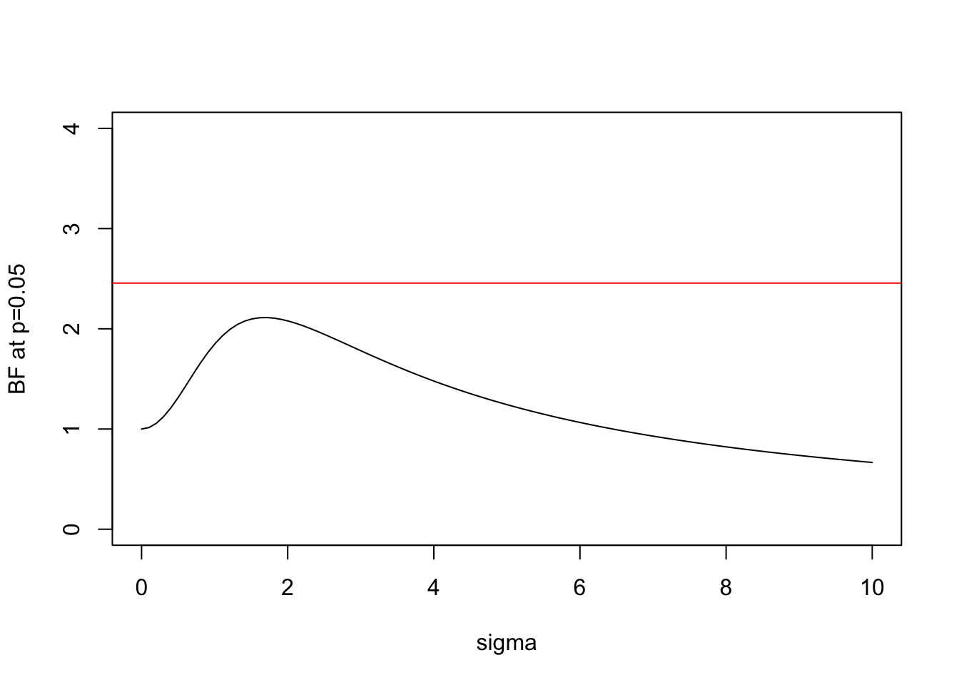
| Version | Author | Date |
|---|---|---|
| c3b365a | John Blischak | 2017-01-02 |
Here the horizontal line shows the bound on the Bayes Factor computed by Sellke et al.
And here is the same plot for \(x=2.58\) (\(p=0.01\)):
plot(s,BF(2.58,s),xlab="sigma",ylab="BF at p=0.01",type="l",ylim=c(0,10))
abline(h=BFbound(0.01),col=2)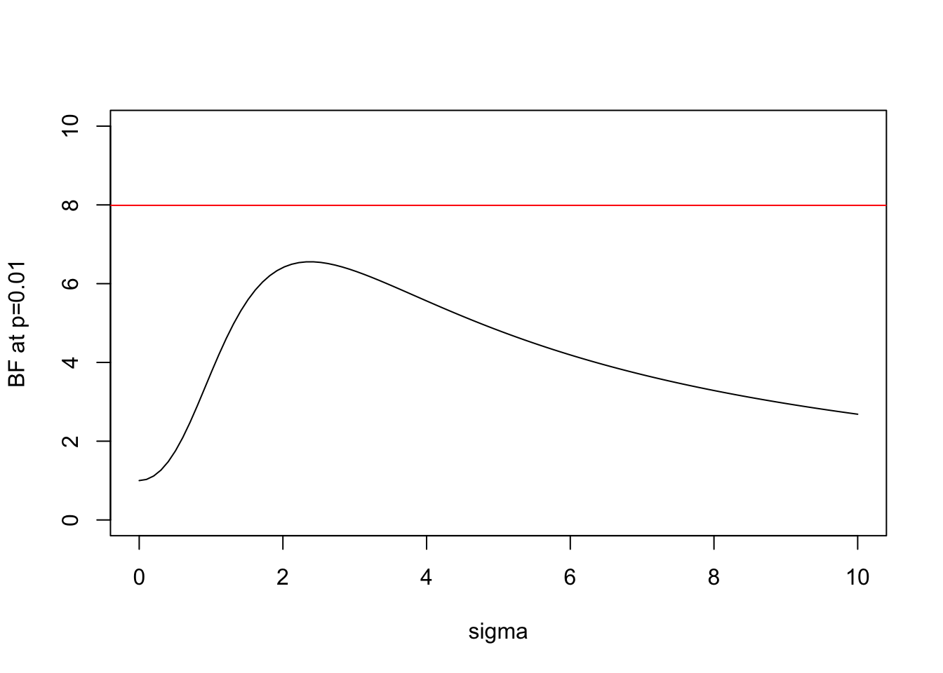
| Version | Author | Date |
|---|---|---|
| c3b365a | John Blischak | 2017-01-02 |
Note some key features:
- In both cases the BF is below the bound given by Sellke et al, as expected.
- As \(\sigma\) increases from 0 the BF is initially 1, rises to a maximum, and then gradually decays. This behavior, which occurs for any \(x\), perhaps helps provide intuition into why it is even possible to derive an upper bound.
- In the limit as \(\sigma \rightarrow \infty\) it is easy to show that (for any \(x\)) the BF \(\rightarrow 0\). This is an example of “Bartlett’s paradox”, and illustrates why you should not just use a “very flat” prior for \(\theta\) under \(H_1\): the Bayes Factor will depend on how flat you mean by “very flat”, and in the limit will always favor \(H_0\).
References
Thomas Sellke, James O. Berger, M. J. Bayarri. 2001. “Calibration of \(p\) Values for Testing Precise Null Hypothesis.” The American Statistician 55 (1).
sessionInfo()R version 3.5.2 (2018-12-20)
Platform: x86_64-apple-darwin15.6.0 (64-bit)
Running under: macOS Mojave 10.14.1
Matrix products: default
BLAS: /Library/Frameworks/R.framework/Versions/3.5/Resources/lib/libRblas.0.dylib
LAPACK: /Library/Frameworks/R.framework/Versions/3.5/Resources/lib/libRlapack.dylib
locale:
[1] en_US.UTF-8/en_US.UTF-8/en_US.UTF-8/C/en_US.UTF-8/en_US.UTF-8
attached base packages:
[1] stats graphics grDevices utils datasets methods base
loaded via a namespace (and not attached):
[1] workflowr_1.2.0 Rcpp_1.0.0 digest_0.6.18 rprojroot_1.3-2
[5] backports_1.1.3 git2r_0.24.0 magrittr_1.5 evaluate_0.12
[9] stringi_1.2.4 fs_1.2.6 whisker_0.3-2 rmarkdown_1.11
[13] tools_3.5.2 stringr_1.3.1 glue_1.3.0 xfun_0.4
[17] yaml_2.2.0 compiler_3.5.2 htmltools_0.3.6 knitr_1.21 This site was created with R Markdown