Summarizing and Interpreting the Posterior (analytic)
Matthew Stephens
2017-01-28
Last updated: 2019-03-31
Checks: 6 0
Knit directory: fiveMinuteStats/analysis/
This reproducible R Markdown analysis was created with workflowr (version 1.2.0). The Report tab describes the reproducibility checks that were applied when the results were created. The Past versions tab lists the development history.
Great! Since the R Markdown file has been committed to the Git repository, you know the exact version of the code that produced these results.
Great job! The global environment was empty. Objects defined in the global environment can affect the analysis in your R Markdown file in unknown ways. For reproduciblity it’s best to always run the code in an empty environment.
The command set.seed(12345) was run prior to running the code in the R Markdown file. Setting a seed ensures that any results that rely on randomness, e.g. subsampling or permutations, are reproducible.
Great job! Recording the operating system, R version, and package versions is critical for reproducibility.
Nice! There were no cached chunks for this analysis, so you can be confident that you successfully produced the results during this run.
Great! You are using Git for version control. Tracking code development and connecting the code version to the results is critical for reproducibility. The version displayed above was the version of the Git repository at the time these results were generated.
Note that you need to be careful to ensure that all relevant files for the analysis have been committed to Git prior to generating the results (you can use wflow_publish or wflow_git_commit). workflowr only checks the R Markdown file, but you know if there are other scripts or data files that it depends on. Below is the status of the Git repository when the results were generated:
Ignored files:
    Ignored:    .Rhistory
    Ignored:    .Rproj.user/
    Ignored:    analysis/.Rhistory
    Ignored:    analysis/bernoulli_poisson_process_cache/

Untracked files:
    Untracked:  _workflowr.yml
    Untracked:  analysis/CI.Rmd
    Untracked:  analysis/gibbs_structure.Rmd
    Untracked:  analysis/libs/
    Untracked:  analysis/results.Rmd
    Untracked:  analysis/shiny/tester/
    Untracked:  docs/MH_intro_files/
    Untracked:  docs/citations.bib
    Untracked:  docs/figure/MH_intro.Rmd/
    Untracked:  docs/figure/hmm.Rmd/
    Untracked:  docs/hmm_files/
    Untracked:  docs/libs/
    Untracked:  docs/shiny/tester/
Note that any generated files, e.g. HTML, png, CSS, etc., are not included in this status report because it is ok for generated content to have uncommitted changes.
These are the previous versions of the R Markdown and HTML files. If you’ve configured a remote Git repository (see ?wflow_git_remote), click on the hyperlinks in the table below to view them.
| File | Version | Author | Date | Message |
|---|---|---|---|---|
| html | 34bcc51 | John Blischak | 2017-03-06 | Build site. |
| Rmd | 5fbc8b5 | John Blischak | 2017-03-06 | Update workflowr project with wflow_update (version 0.4.0). |
| html | fb0f6e3 | stephens999 | 2017-03-03 | Merge pull request #33 from mdavy86/f/review |
| html | 0713277 | stephens999 | 2017-03-03 | Merge pull request #31 from mdavy86/f/review |
| Rmd | d674141 | Marcus Davy | 2017-02-27 | typos, refs |
| html | dc8a1bb | stephens999 | 2017-01-28 | add html, figs |
| Rmd | c3e49d5 | stephens999 | 2017-01-28 | Files commited by wflow_commit. |
Overview
This vignette illustrates how to summarize and interpret a posterior distribution that has been computed analytically.
You should be familiar with simple analytic calculations of the posterior distribution of a parameter, such as for a binomial proportion.
Summarising and interpreting a posterior
Suppose we have a parameter \(q\), whose posterior distribution we have computed to be Beta(31, 71) (as here for example). What does this mean? What statements can we make about \(q\)? How do we obtain interval estimates and point estimates for \(q\)?
Remember that the posterior distribution represents our uncertainty (or certainty) in \(q\), after combining the information in the data (the likelihood) with what we knew before collecting data (the prior).
To get some intuition, we could plot the posterior distribution so we can see what it looks like.
q = seq(0,1,length=100)
plot(q, dbeta(q, 31,71), main="Posterior for $q$", ylab="density", type="l")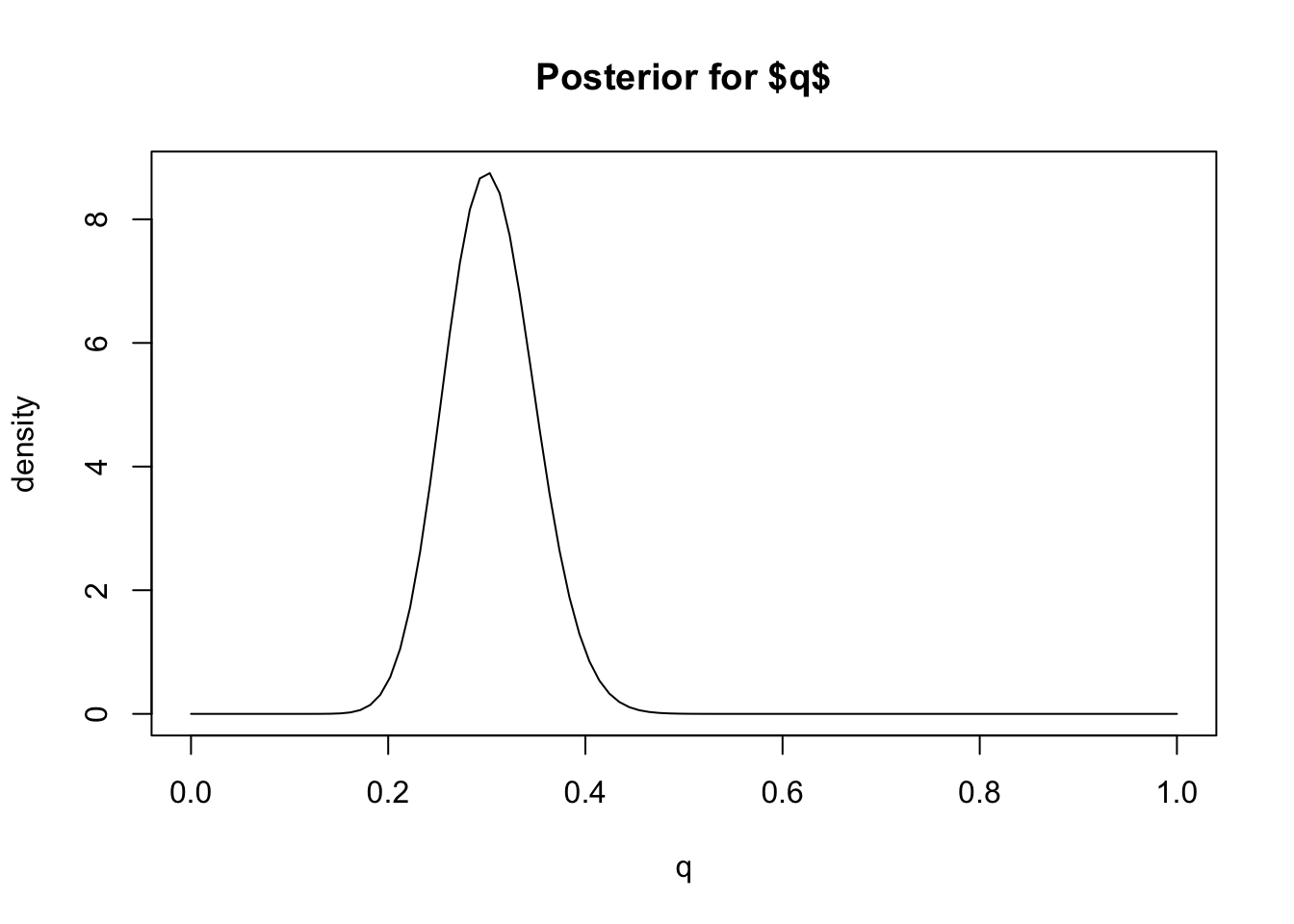
Based on this plot we can visually see that this posterior distribution has the property that \(q\) is highly likely to be less than 0.4 (say) because most of the mass of the distribution lies below 0.4. In Bayesian inference we quantify statements like this – that a particular event is “highly likely” – by computing the “posterior probability” of the event, which is the probability of the event under the posterior distribution.
For example, in this case we can compute the (posterior) probability that \(q<0.4\), or \(\Pr(q <0.4 | D)\). Since we know the posterior distribution is a Be(31,71) distribution, this probability is easy to compute using the pbeta function:
pbeta(0.4,31,71)[1] 0.9792202So we would say “The posterior probability that \(q<0.4\) is 0.98”.
Interval estimates
We can extend this idea to assess the certainty (or confidence) that \(q\) lies in any interval. For example, from the plot it looks like \(q\) will very likely lie in the interval [0.2,0.4] because most of the posterior distribution mass lies between these two numbers. To quantify how likely we compute the (posterior) probability that \(q\) lies in the interval \([0.2,0.4]\), \(\Pr(q \in [0.2,0.4] | D)\). Again, this can be computed using the pbeta function:
pbeta(0.4,31,71) - pbeta(0.2,31,71)[1] 0.9721229Thus, based on our prior and the data, we would be highly confident (probability approximately 97%) that \(q\) lies between 0.2 and 0.4. That is, \([0.2,0.4]\) is a 97% Bayesian Confidence Interval for \(q\). (Bayesian Confidence Intervals are often referred to as “Credible Intervals”, and also often abbreviated to CI.)
In practice, it is more common to compute Bayesian Confidence Intervals the other way around: specify the level of confidence we want to achieve and find an interval that achieves that level of confidence. This can be done by computing the quantiles of the posterior distribution. For example, the 0.05 and 0.95 quantiles of the posterior would define a 90% Bayesian Confidence Interval.
In our example, these quantiles of the Beta distribution can be computed using the qbeta function, like this:
qbeta(0.05,31,71)[1] 0.2315858qbeta(0.95,31,71)[1] 0.38065So [0.23, 0.38] is a 90% Bayesian Confidence Interval for \(q\). (It is 90% because there is a 5% chance of it being above 0.23 and 5% of it being above 0.38).
Point Estimates
In some cases we might be happy to give our “best guess” for \(q\), rather than worrying about our uncertainty. That is, we might be interested in giving a “point estimate” for \(q\). Essentially this boils down to summarizing the posterior distribution by a single number.
When \(q\) is a continuous-valued variable, as here, the most common Bayesian point estimate is the mean (or expectation) of the posterior distribution, which is called the “posterior mean”. The mean of the Beta(31,71) distribution is 31/(31+71) = 0.3. So we would say “The posterior mean for \(q\) is 0.3.”
An alternative to the mean is the median. The median of the Beta(31,71) distribution can be found using qbeta:
qbeta(0.5, 31,71)[1] 0.3026356So we would say “The posterior median for \(q\) is 0.3”.
The mode of the posterior (“posterior mode”) is another possible summary, although this perhaps makes more sense in settings where \(q\) is a discrete variable rather than a continuous variable as here.
Summary
The most common summaries of a posterior distribution are interval estimates and point estimates.
Interval estimates can be obtained by computing quantiles of the posterior distribution. Bayesian Confidence intervals are often called “Credible Intervals”.
Point estimates are typically obtained by computing the mean or median (or mode) of the posterior distribution. These are called the “posterior mean” or the “posterior median” (or “posterior mode”).
Exercise
Suppose you are interested in a parameter \(\theta\) and obtain a posterior distribution for \(\theta\) to be normal with mean 0.2 and standard deviation 0.4. Find
- a 90% Credible Interval for \(\theta\).
- a 95% Credible Interval for \(\theta\).
- a point estimate for \(\theta\).
sessionInfo()R version 3.5.2 (2018-12-20)
Platform: x86_64-apple-darwin15.6.0 (64-bit)
Running under: macOS Mojave 10.14.1
Matrix products: default
BLAS: /Library/Frameworks/R.framework/Versions/3.5/Resources/lib/libRblas.0.dylib
LAPACK: /Library/Frameworks/R.framework/Versions/3.5/Resources/lib/libRlapack.dylib
locale:
[1] en_US.UTF-8/en_US.UTF-8/en_US.UTF-8/C/en_US.UTF-8/en_US.UTF-8
attached base packages:
[1] stats graphics grDevices utils datasets methods base
loaded via a namespace (and not attached):
[1] workflowr_1.2.0 Rcpp_1.0.0 digest_0.6.18 rprojroot_1.3-2
[5] backports_1.1.3 git2r_0.24.0 magrittr_1.5 evaluate_0.12
[9] stringi_1.2.4 fs_1.2.6 whisker_0.3-2 rmarkdown_1.11
[13] tools_3.5.2 stringr_1.3.1 glue_1.3.0 xfun_0.4
[17] yaml_2.2.0 compiler_3.5.2 htmltools_0.3.6 knitr_1.21 This site was created with R Markdown