fastica_centered
Matthew Stephens
2025-11-14
Last updated: 2025-11-17
Checks: 7 0
Knit directory: misc/analysis/
This reproducible R Markdown analysis was created with workflowr (version 1.7.1). The Checks tab describes the reproducibility checks that were applied when the results were created. The Past versions tab lists the development history.
Great! Since the R Markdown file has been committed to the Git repository, you know the exact version of the code that produced these results.
Great job! The global environment was empty. Objects defined in the global environment can affect the analysis in your R Markdown file in unknown ways. For reproduciblity it’s best to always run the code in an empty environment.
The command set.seed(1) was run prior to running the
code in the R Markdown file. Setting a seed ensures that any results
that rely on randomness, e.g. subsampling or permutations, are
reproducible.
Great job! Recording the operating system, R version, and package versions is critical for reproducibility.
Nice! There were no cached chunks for this analysis, so you can be confident that you successfully produced the results during this run.
Great job! Using relative paths to the files within your workflowr project makes it easier to run your code on other machines.
Great! You are using Git for version control. Tracking code development and connecting the code version to the results is critical for reproducibility.
The results in this page were generated with repository version 80ad636. See the Past versions tab to see a history of the changes made to the R Markdown and HTML files.
Note that you need to be careful to ensure that all relevant files for
the analysis have been committed to Git prior to generating the results
(you can use wflow_publish or
wflow_git_commit). workflowr only checks the R Markdown
file, but you know if there are other scripts or data files that it
depends on. Below is the status of the Git repository when the results
were generated:
Ignored files:
    Ignored:    .DS_Store
    Ignored:    .Rhistory
    Ignored:    .Rproj.user/
    Ignored:    analysis/.RData
    Ignored:    analysis/.Rhistory
    Ignored:    analysis/ALStruct_cache/
    Ignored:    analysis/figure/
    Ignored:    data/.Rhistory
    Ignored:    data/methylation-data-for-matthew.rds
    Ignored:    data/pbmc/
    Ignored:    data/pbmc_purified.RData

Untracked files:
    Untracked:  .dropbox
    Untracked:  Icon
    Untracked:  analysis/GHstan.Rmd
    Untracked:  analysis/GTEX-cogaps.Rmd
    Untracked:  analysis/PACS.Rmd
    Untracked:  analysis/Rplot.png
    Untracked:  analysis/SPCAvRP.rmd
    Untracked:  analysis/abf_comparisons.Rmd
    Untracked:  analysis/admm_02.Rmd
    Untracked:  analysis/admm_03.Rmd
    Untracked:  analysis/bispca.Rmd
    Untracked:  analysis/cache/
    Untracked:  analysis/cholesky.Rmd
    Untracked:  analysis/compare-transformed-models.Rmd
    Untracked:  analysis/cormotif.Rmd
    Untracked:  analysis/cp_ash.Rmd
    Untracked:  analysis/eQTL.perm.rand.pdf
    Untracked:  analysis/eb_power2.Rmd
    Untracked:  analysis/eb_prepilot.Rmd
    Untracked:  analysis/eb_var.Rmd
    Untracked:  analysis/ebpmf1.Rmd
    Untracked:  analysis/ebpmf_sla_text.Rmd
    Untracked:  analysis/ebspca_sims.Rmd
    Untracked:  analysis/explore_psvd.Rmd
    Untracked:  analysis/fa_check_identify.Rmd
    Untracked:  analysis/fa_iterative.Rmd
    Untracked:  analysis/fastica_heated.Rmd
    Untracked:  analysis/flash_cov_overlapping_groups_init.Rmd
    Untracked:  analysis/flash_test_tree.Rmd
    Untracked:  analysis/flashier_newgroups.Rmd
    Untracked:  analysis/flashier_nmf_triples.Rmd
    Untracked:  analysis/flashier_pbmc.Rmd
    Untracked:  analysis/flashier_snn_shifted_prior.Rmd
    Untracked:  analysis/greedy_ebpmf_exploration_00.Rmd
    Untracked:  analysis/ieQTL.perm.rand.pdf
    Untracked:  analysis/lasso_em_03.Rmd
    Untracked:  analysis/m6amash.Rmd
    Untracked:  analysis/mash_bhat_z.Rmd
    Untracked:  analysis/mash_ieqtl_permutations.Rmd
    Untracked:  analysis/methylation_example.Rmd
    Untracked:  analysis/mixsqp.Rmd
    Untracked:  analysis/mr.ash_lasso_init.Rmd
    Untracked:  analysis/mr.mash.test.Rmd
    Untracked:  analysis/mr_ash_modular.Rmd
    Untracked:  analysis/mr_ash_parameterization.Rmd
    Untracked:  analysis/mr_ash_ridge.Rmd
    Untracked:  analysis/mv_gaussian_message_passing.Rmd
    Untracked:  analysis/nejm.Rmd
    Untracked:  analysis/nmf_bg.Rmd
    Untracked:  analysis/nonneg_underapprox.Rmd
    Untracked:  analysis/normal_conditional_on_r2.Rmd
    Untracked:  analysis/normalize.Rmd
    Untracked:  analysis/pbmc.Rmd
    Untracked:  analysis/pca_binary_weighted.Rmd
    Untracked:  analysis/pca_l1.Rmd
    Untracked:  analysis/poisson_nmf_approx.Rmd
    Untracked:  analysis/poisson_shrink.Rmd
    Untracked:  analysis/poisson_transform.Rmd
    Untracked:  analysis/qrnotes.txt
    Untracked:  analysis/ridge_iterative_02.Rmd
    Untracked:  analysis/ridge_iterative_splitting.Rmd
    Untracked:  analysis/samps/
    Untracked:  analysis/sc_bimodal.Rmd
    Untracked:  analysis/shrinkage_comparisons_changepoints.Rmd
    Untracked:  analysis/susie_cov.Rmd
    Untracked:  analysis/susie_en.Rmd
    Untracked:  analysis/susie_z_investigate.Rmd
    Untracked:  analysis/svd-timing.Rmd
    Untracked:  analysis/temp.RDS
    Untracked:  analysis/temp.Rmd
    Untracked:  analysis/test-figure/
    Untracked:  analysis/test.Rmd
    Untracked:  analysis/test.Rpres
    Untracked:  analysis/test.md
    Untracked:  analysis/test_qr.R
    Untracked:  analysis/test_sparse.Rmd
    Untracked:  analysis/tree_dist_top_eigenvector.Rmd
    Untracked:  analysis/z.txt
    Untracked:  code/coordinate_descent_symNMF.R
    Untracked:  code/multivariate_testfuncs.R
    Untracked:  code/rqb.hacked.R
    Untracked:  data/4matthew/
    Untracked:  data/4matthew2/
    Untracked:  data/E-MTAB-2805.processed.1/
    Untracked:  data/ENSG00000156738.Sim_Y2.RDS
    Untracked:  data/GDS5363_full.soft.gz
    Untracked:  data/GSE41265_allGenesTPM.txt
    Untracked:  data/Muscle_Skeletal.ACTN3.pm1Mb.RDS
    Untracked:  data/P.rds
    Untracked:  data/Thyroid.FMO2.pm1Mb.RDS
    Untracked:  data/bmass.HaemgenRBC2016.MAF01.Vs2.MergedDataSources.200kRanSubset.ChrBPMAFMarkerZScores.vs1.txt.gz
    Untracked:  data/bmass.HaemgenRBC2016.Vs2.NewSNPs.ZScores.hclust.vs1.txt
    Untracked:  data/bmass.HaemgenRBC2016.Vs2.PreviousSNPs.ZScores.hclust.vs1.txt
    Untracked:  data/eb_prepilot/
    Untracked:  data/finemap_data/fmo2.sim/b.txt
    Untracked:  data/finemap_data/fmo2.sim/dap_out.txt
    Untracked:  data/finemap_data/fmo2.sim/dap_out2.txt
    Untracked:  data/finemap_data/fmo2.sim/dap_out2_snp.txt
    Untracked:  data/finemap_data/fmo2.sim/dap_out_snp.txt
    Untracked:  data/finemap_data/fmo2.sim/data
    Untracked:  data/finemap_data/fmo2.sim/fmo2.sim.config
    Untracked:  data/finemap_data/fmo2.sim/fmo2.sim.k
    Untracked:  data/finemap_data/fmo2.sim/fmo2.sim.k4.config
    Untracked:  data/finemap_data/fmo2.sim/fmo2.sim.k4.snp
    Untracked:  data/finemap_data/fmo2.sim/fmo2.sim.ld
    Untracked:  data/finemap_data/fmo2.sim/fmo2.sim.snp
    Untracked:  data/finemap_data/fmo2.sim/fmo2.sim.z
    Untracked:  data/finemap_data/fmo2.sim/pos.txt
    Untracked:  data/logm.csv
    Untracked:  data/m.cd.RDS
    Untracked:  data/m.cdu.old.RDS
    Untracked:  data/m.new.cd.RDS
    Untracked:  data/m.old.cd.RDS
    Untracked:  data/mainbib.bib.old
    Untracked:  data/mat.csv
    Untracked:  data/mat.txt
    Untracked:  data/mat_new.csv
    Untracked:  data/matrix_lik.rds
    Untracked:  data/paintor_data/
    Untracked:  data/running_data_chris.csv
    Untracked:  data/running_data_matthew.csv
    Untracked:  data/temp.txt
    Untracked:  data/y.txt
    Untracked:  data/y_f.txt
    Untracked:  data/zscore_jointLCLs_m6AQTLs_susie_eQTLpruned.rds
    Untracked:  data/zscore_jointLCLs_random.rds
    Untracked:  explore_udi.R
    Untracked:  output/fit.k10.rds
    Untracked:  output/fit.nn.pbmc.purified.rds
    Untracked:  output/fit.nn.rds
    Untracked:  output/fit.nn.s.001.rds
    Untracked:  output/fit.nn.s.01.rds
    Untracked:  output/fit.nn.s.1.rds
    Untracked:  output/fit.nn.s.10.rds
    Untracked:  output/fit.snn.s.001.rds
    Untracked:  output/fit.snn.s.01.nninit.rds
    Untracked:  output/fit.snn.s.01.rds
    Untracked:  output/fit.varbvs.RDS
    Untracked:  output/fit2.nn.pbmc.purified.rds
    Untracked:  output/glmnet.fit.RDS
    Untracked:  output/snn07.txt
    Untracked:  output/snn34.txt
    Untracked:  output/test.bv.txt
    Untracked:  output/test.gamma.txt
    Untracked:  output/test.hyp.txt
    Untracked:  output/test.log.txt
    Untracked:  output/test.param.txt
    Untracked:  output/test2.bv.txt
    Untracked:  output/test2.gamma.txt
    Untracked:  output/test2.hyp.txt
    Untracked:  output/test2.log.txt
    Untracked:  output/test2.param.txt
    Untracked:  output/test3.bv.txt
    Untracked:  output/test3.gamma.txt
    Untracked:  output/test3.hyp.txt
    Untracked:  output/test3.log.txt
    Untracked:  output/test3.param.txt
    Untracked:  output/test4.bv.txt
    Untracked:  output/test4.gamma.txt
    Untracked:  output/test4.hyp.txt
    Untracked:  output/test4.log.txt
    Untracked:  output/test4.param.txt
    Untracked:  output/test5.bv.txt
    Untracked:  output/test5.gamma.txt
    Untracked:  output/test5.hyp.txt
    Untracked:  output/test5.log.txt
    Untracked:  output/test5.param.txt

Unstaged changes:
    Modified:   .gitignore
    Modified:   analysis/eb_snmu.Rmd
    Modified:   analysis/ebnm_binormal.Rmd
    Modified:   analysis/ebpower.Rmd
    Modified:   analysis/flashier_log1p.Rmd
    Modified:   analysis/flashier_sla_text.Rmd
    Modified:   analysis/logistic_z_scores.Rmd
    Modified:   analysis/mr_ash_pen.Rmd
    Modified:   analysis/nmu_em.Rmd
    Modified:   analysis/susie_flash.Rmd
    Modified:   analysis/tap_free_energy.Rmd
    Modified:   misc.Rproj
Note that any generated files, e.g. HTML, png, CSS, etc., are not included in this status report because it is ok for generated content to have uncommitted changes.
These are the previous versions of the repository in which changes were
made to the R Markdown (analysis/fastica_centered.Rmd) and
HTML (docs/fastica_centered.html) files. If you’ve
configured a remote Git repository (see ?wflow_git_remote),
click on the hyperlinks in the table below to view the files as they
were in that past version.
| File | Version | Author | Date | Message |
|---|---|---|---|---|
| Rmd | 80ad636 | Matthew Stephens | 2025-11-17 | workflowr::wflow_publish("analysis/fastica_centered.Rmd") |
| html | 7afc85f | Matthew Stephens | 2025-11-16 | Build site. |
| Rmd | bd2737c | Matthew Stephens | 2025-11-16 | workflowr::wflow_publish("fastica_centered.Rmd") |
| html | 9584c9b | Matthew Stephens | 2025-11-14 | Build site. |
| Rmd | 58374e8 | Matthew Stephens | 2025-11-14 | workflowr::wflow_publish("fastica_centered.Rmd") |
Introduction
I found previously that the original fastICA algorithm seems to have trouble finding groups that are unbalanced. I believe that this is because the log-cosh objective function favours symmetry. ie maximizing or minimizing \(\log \cosh (X'w)\) (subject to \(w'w=1\), which implies ||X’w||= 1 if \(XX'=I\)) tends to find symmetric \(X'w\). I want to try to fix this using an intercept. That is, maximize \(\log \cosh (X'w + c)\) over both \(w\) and \(c\).
I gave Gemini this problem and it gave me the following response and code.
“This adds a new parameter, \(c\), that we also need to optimize. We can derive the update rules by taking the partial derivatives of the objective function (negentropy approximation) with respect to both \(w\) and \(c\) and setting them to zero (this is the Karush-Kuhn-Tucker or KKT-based approach).
This gives us two conditions to satisfy:
For \(w\): \(E[X g(w^TX + c)] - \lambda w = 0\)
For \(c\): \(E[g(w^TX + c)] = 0\)
Where \(g\) is your contrast function (\(\tanh\)) and \(\lambda\) is a scalar (Lagrange multiplier).
Condition (2) is new and very intuitive: it means the algorithm must find an intercept \(c\) that “centers” the transformed projection \(g(P)\) to have a mean of zero. This leads to a simple two-step update within each iteration:
Update c: First, for a fixed w, find the c that solves \(E[g(w^TX + c)] = 0\).
Update w: Then, using that new c, perform the standard FastICA update for w.”
#' Single-unit FastICA update with an intercept term 'c'
#'
#' @param X The pre-processed (centered and whitened) data matrix (p x n).
#' @param w The current weight vector (p x 1).
#' @param c The current intercept scalar.
#' @param c_update_steps How many Newton steps to take for 'c' per iteration.
#'                       1 is usually sufficient.
#' @return A list containing the updated 'w' (unnormalized) and 'c'.

fastica_r1update_wc = function(X, w, c, c_update_steps = 1) {

  # 1. Normalize w (as before)
  w = w / sqrt(sum(w^2))

  # --- Step 1: Update the intercept 'c' ---

  # Get the current projection *without* the intercept
  # P_current is an (n x 1) vector
  P_current = as.vector(t(X) %*% w)

  # We want to find 'c' that solves E[g(P_current + c)] = 0
  # We use one (or more) Newton steps: c_new = c - f(c) / f'(c)

  for (i in 1:c_update_steps) {
    P_shifted = P_current + c

    # g(P_current + c)
    G_c = tanh(P_shifted)

    # g'(P_current + c)
    G2_c = 1 - tanh(P_shifted)^2

    # E[g(P_current + c)]
    mean_G = mean(G_c)

    # E[g'(P_current + c)]
    mean_G2 = mean(G2_c)

    # The Newton step (add epsilon for stability)
    c = c - mean_G / (mean_G2 + 1e-6)
  }

  # --- Step 2: Update the weight vector 'w' ---

  # Now we use the *updated* 'c' to update 'w'
  # P = w'X + c (using the new 'c' from Step 1)
  P = P_current + c

  # g(P)
  G = tanh(P)

  # g'(P)
  G2 = 1 - tanh(P)^2

  # The FastICA update rule for 'w':
  # w_new = E[X * g(P)] - E[g'(P)] * w
  # (Note: We use sum(G2) as an estimate for E[g'(P)] * n)
  # (and X %*% G as an estimate for E[X*g(P)] * n)
  # The 'n' scaling factor cancels, as 'w' is normalized next iteration.
  w_new = X %*% G - sum(G2) * w

  # 4. Return the updated vector and intercept
  return(list(w = w_new, c = c))
}

#'
#' This is the function that the "profiled" and "skew" update rules
#' are trying to find an extremum (max/min) of.
#'
#' @param X The pre-processed (centered and whitened) data matrix (p x n).
#' @param w The weight vector (p x 1).
#' @param c The intercept scalar.
#' @return The scalar value of the objective function.

compute_objective = function(X, w, c) {

  # 1. Normalize w to stay on the ||w||=1 constraint
  w = w / sqrt(sum(w^2))

  # 2. Calculate the projection
  P = as.vector(t(X) %*% w) # (n x 1) vector

  # 3. Create the shifted projection
  S = P + c

  # 5. Apply G(u) = log(cosh(u))
  G_S = log(cosh(S))

  # 6. Compute the expectation (as a sample mean)
  objective_value = mean(G_S)

  return(objective_value)
}
Preprocessing code
preprocess = function(X, n.comp=10){
  n <- nrow(X)
  p <- ncol(X)
  X <- scale(X, scale = FALSE)
  X <- t(X)

  ## This appears to be equivalant to X1 = t(svd(X)$v[,1:n.comp])
  V <- X %*% t(X)/n
  s <- La.svd(V)
  D <- diag(c(1/sqrt(s$d)))
  K <- D %*% t(s$u)
  K <- matrix(K[1:n.comp, ], n.comp, p)
  X1 <- K %*% X
  return(X1)
}
Simulate data: 3 small groups
Here I simulate 3 groups, with only 20 members each, which I previously found that fastICA had trouble with.
K=3
p = 1000
n = 100
set.seed(1)
L = matrix(0,nrow=n,ncol=K)
for(i in 1:K){L[sample(1:n,20),i]=1}
FF = matrix(rnorm(p*K), nrow = p, ncol=K)

X = L %*% t(FF) + rnorm(n*p,0,0.01)
plot(X %*% FF[,1])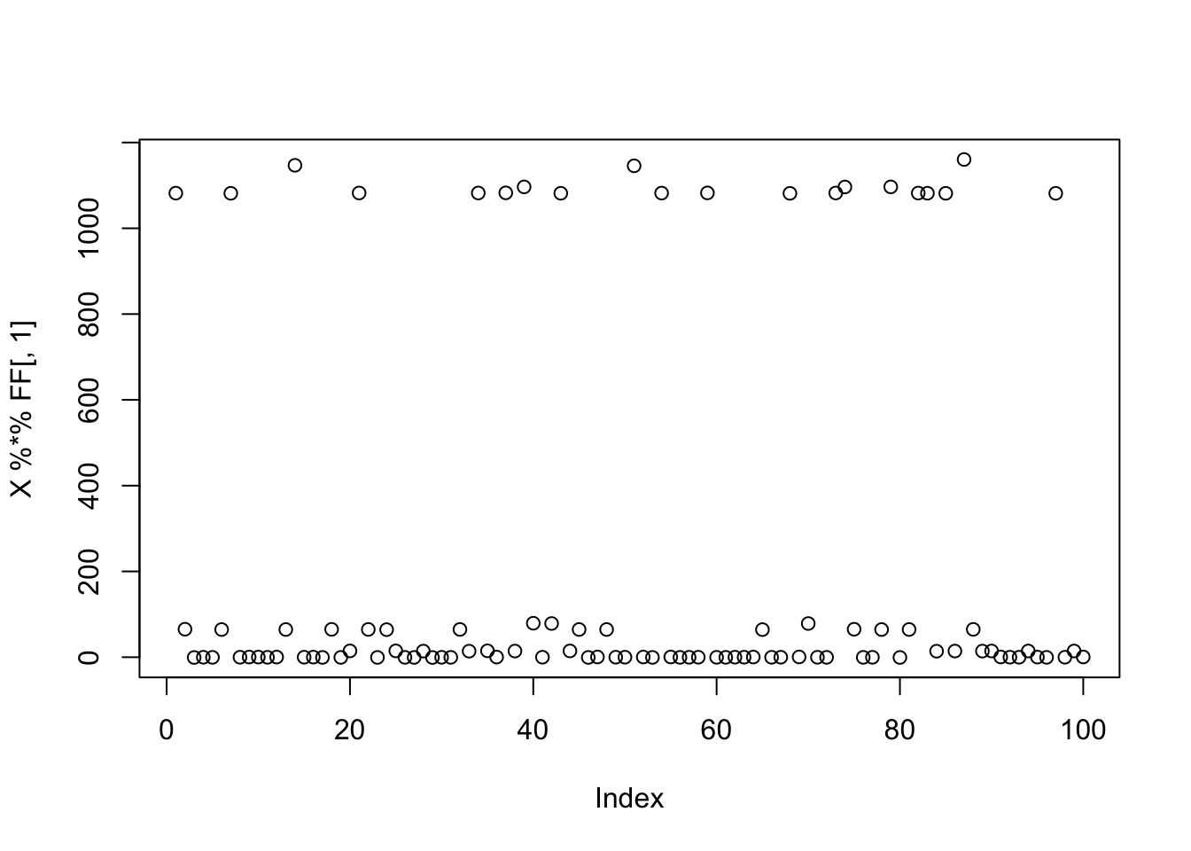
| Version | Author | Date |
|---|---|---|
| 9584c9b | Matthew Stephens | 2025-11-14 |
centered fastICA (random start)
When I initialize these new updates with a random w, it does not pick out a single source:
X1 = preprocess(X)
w = rnorm(nrow(X1))
c = 0 # this does not matter as c is updated first
res = list(w=w,c=c)
for(i in 1:100)
  res = fastica_r1update_wc(X1,res$w,res$c)
cor(L,t(X1) %*% res$w)
[,1]
[1,] -0.2146838
[2,] -0.1209332
[3,] 0.3947973plot(as.vector(t(X1) %*% res$w))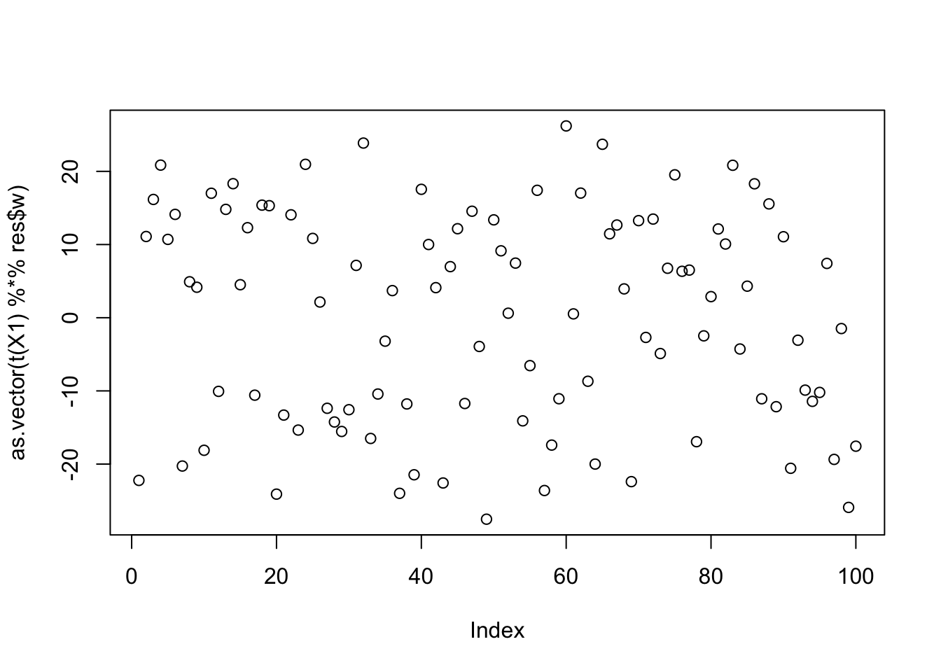
| Version | Author | Date |
|---|---|---|
| 9584c9b | Matthew Stephens | 2025-11-14 |
res$c[1] -0.03965451compute_objective(X1,res$w,res$c)[1] 0.4035189centered fastICA (true factor start)
Now I try initializing at (or close to) a true factor: it converges to the solution I wanted, and more importantly it has a much higher objective than then random start. This confirms that the changed objective function is having the desired effect.
w = X1 %*% L[,1]
plot(t(X1) %*% w)
| Version | Author | Date |
|---|---|---|
| 9584c9b | Matthew Stephens | 2025-11-14 |
c = 0 # note this does not matter much because c gets updated first in the algorithm
res = list(w=w,c=c)
for(i in 1:100)
  res = fastica_r1update_wc(X1,res$w,res$c)
cor(L,t(X1) %*% res$w)
[,1]
[1,] 9.999997e-01
[2,] -7.339242e-06
[3,] -6.260554e-02plot(as.vector(t(X1) %*% res$w))
| Version | Author | Date |
|---|---|---|
| 9584c9b | Matthew Stephens | 2025-11-14 |
print(compute_objective(X1,res$w,res$c), digits=20)[1] 1.1605289119177262247Try initializing from a different true factor - we see the objective function is almost identical as for the first factor in this case (but slightly lower).
w = X1 %*% L[,2]
plot(t(X1) %*% w)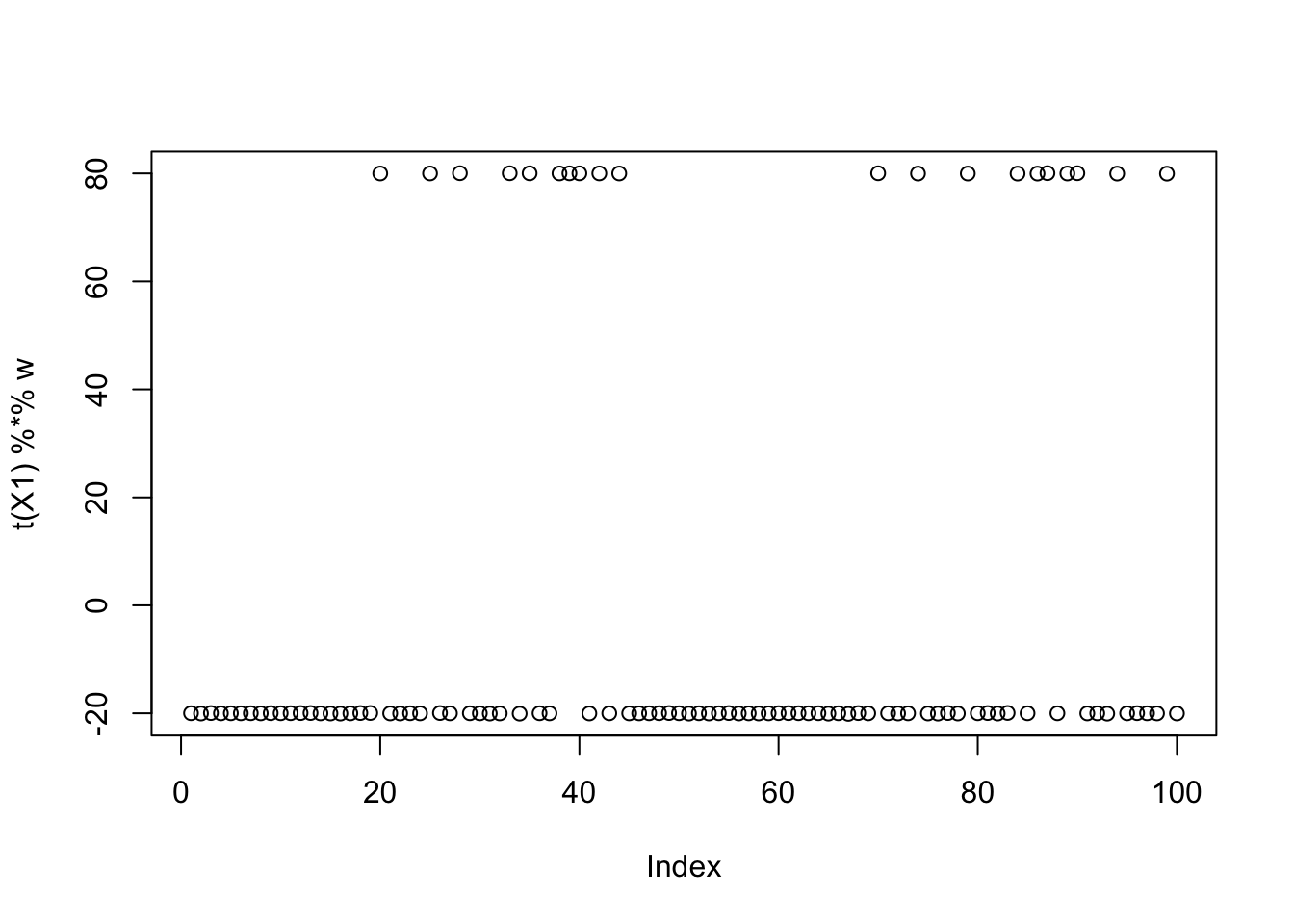
c = 0 # note this does not matter much because c gets updated first in the algorithm
res = list(w=w,c=c)
for(i in 1:100)
  res = fastica_r1update_wc(X1,res$w,res$c)
cor(L,t(X1) %*% res$w)
[,1]
[1,] 2.587794e-05
[2,] 9.999997e-01
[3,] 9.652197e-05plot(as.vector(t(X1) %*% res$w))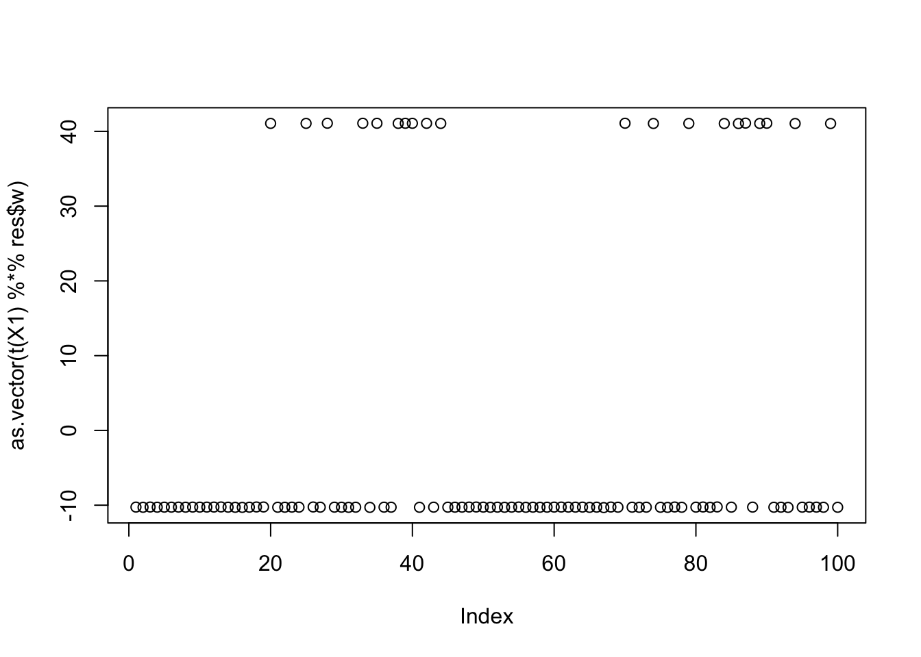
| Version | Author | Date |
|---|---|---|
| 7afc85f | Matthew Stephens | 2025-11-16 |
print(compute_objective(X1,res$w,res$c), digits=20)[1] 1.1605281825359521353Same for the third factor: so the objective function for all 3 factors is approximately equal. This is not a coincidence; in general the objective function for all binary factors of equal size should be approximately equal with this centering approach. (But the objective function will tend to favor unbalanced factors.)
w = X1 %*% L[,3]
plot(t(X1) %*% w)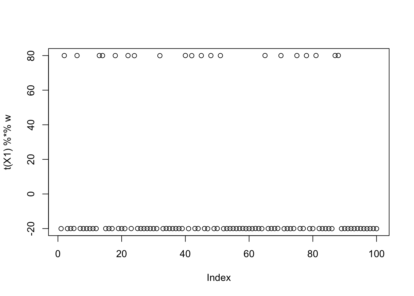
c = 0 # note this does not matter much because c gets updated first in the algorithm
res = list(w=w,c=c)
for(i in 1:100)
  res = fastica_r1update_wc(X1,res$w,res$c)
cor(L,t(X1) %*% res$w)
[,1]
[1,] -6.247381e-02
[2,] 9.005038e-06
[3,] 9.999997e-01plot(as.vector(t(X1) %*% res$w))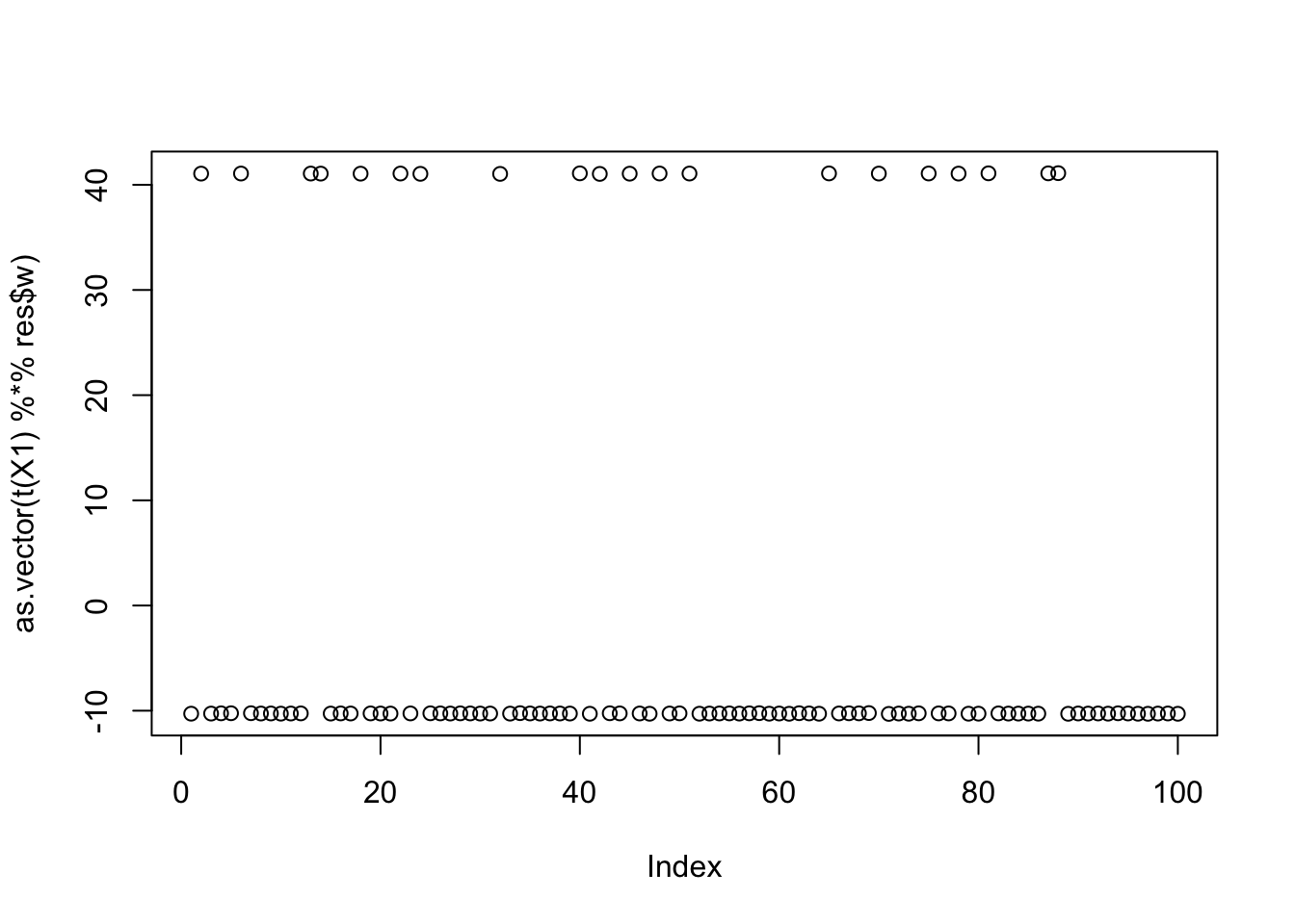
| Version | Author | Date |
|---|---|---|
| 7afc85f | Matthew Stephens | 2025-11-16 |
print(compute_objective(X1,res$w,res$c),digits=20)[1] 1.1605283389603271438centered fastICA (many random starts)
Here I try with 100 random starts - there are lots of different results, and some of them reach objectives similar to that from the true starts.
obj = rep(0,100)
for(seed in 1:100){
  set.seed(seed)
  res = list(w = rnorm(nrow(X1)), c=0)
  for(i in 1:100)
    res = fastica_r1update_wc(X1,res$w,res$c)
  obj[seed] = compute_objective(X1,res$w,res$c)
}
plot(obj)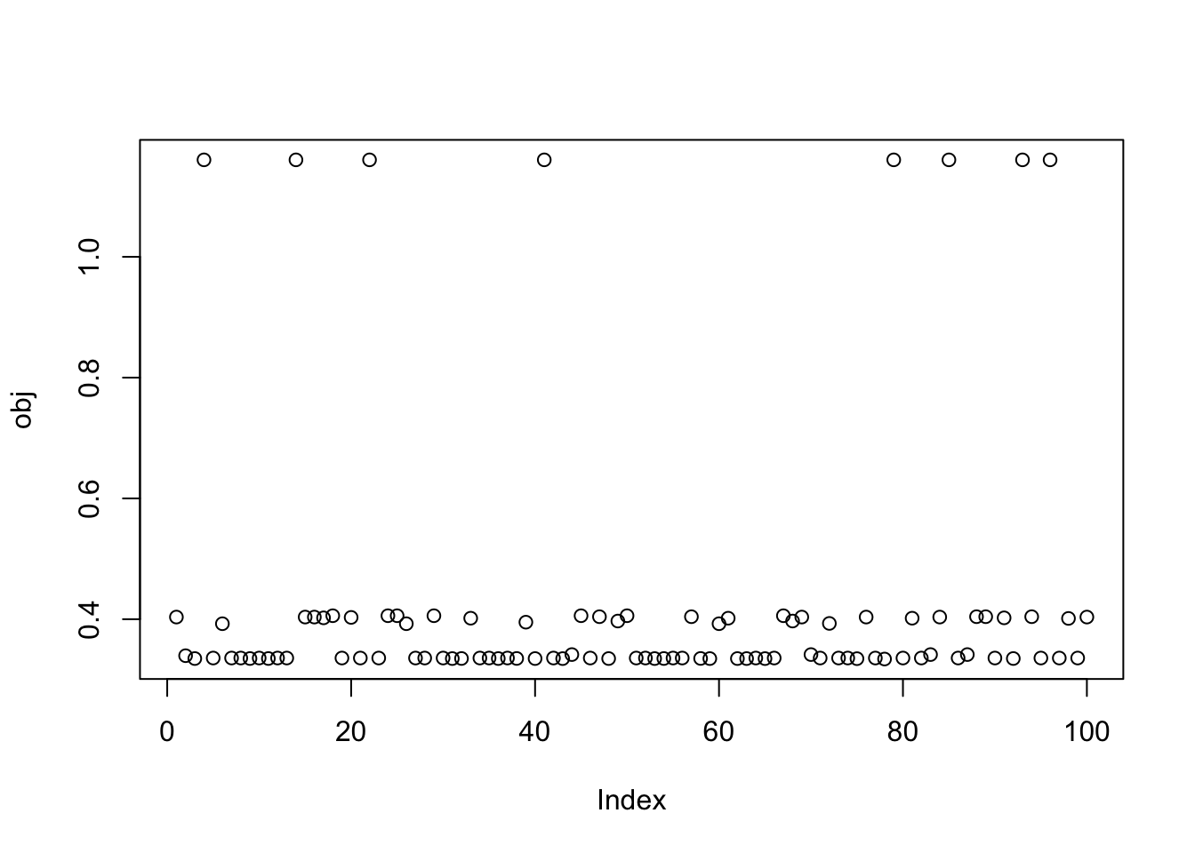
| Version | Author | Date |
|---|---|---|
| 7afc85f | Matthew Stephens | 2025-11-16 |
print(sort(obj,decreasing=TRUE)[1:15],digits=20) [1] 1.16052891191772644675 1.16052891191772622470 1.16052891191772555857
[4] 1.16052833896032758787 1.16052833896032714378 1.16052833894469764608
[7] 1.16052818253595213527 1.16052818253595169118 0.40573150817501507648
[10] 0.40573150817501502097 0.40573150817501502097 0.40573150817501502097
[13] 0.40573150817501496546 0.40573150817501496546 0.40573150817501424381Close inspection of the objective values suggest that the top 7 seeds find the first factor, seeds 8-10 find the third factor, and seeds 11-14 find the second factor. This turns out to be correct! For example, here are the results for the seed achieving the max objective.
seed= order(obj,decreasing=TRUE)[1]
set.seed(seed)
res = list(w = rnorm(nrow(X1)), c=0)
for(i in 1:100)
  res = fastica_r1update_wc(X1,res$w,res$c)
cor(L,t(X1) %*% res$w)
[,1]
[1,] -9.999997e-01
[2,] 7.339242e-06
[3,] 6.260554e-02plot(as.vector(t(X1) %*% res$w))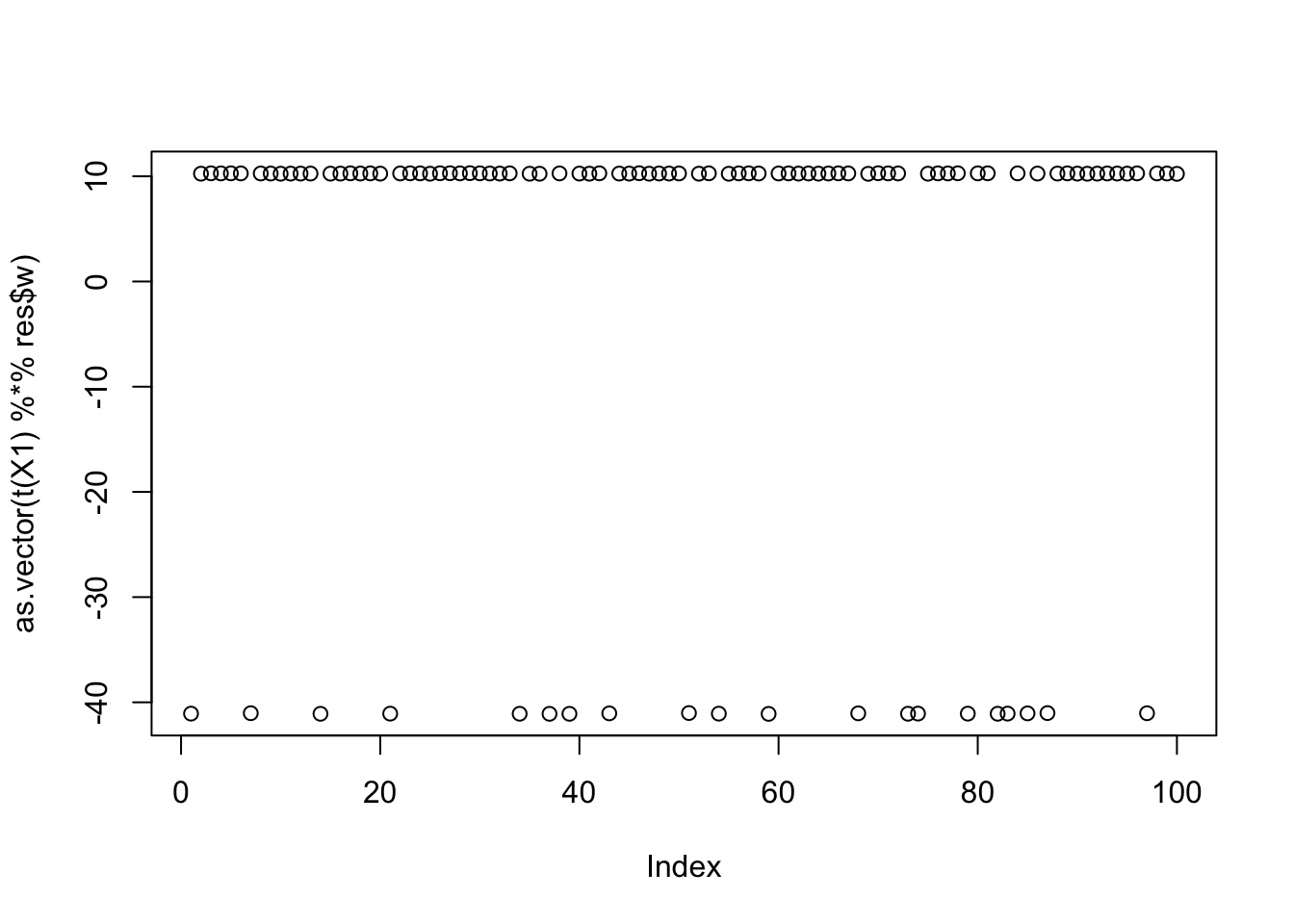
max(obj)[1] 1.160529Here is the seed for the 8th biggest objective (finds the third factor)
seed= order(obj,decreasing=TRUE)[8]
set.seed(seed)
res = list(w = rnorm(nrow(X1)), c=0)
for(i in 1:100)
  res = fastica_r1update_wc(X1,res$w,res$c)
cor(L,t(X1) %*% res$w)
[,1]
[1,] -2.587794e-05
[2,] -9.999997e-01
[3,] -9.652197e-05plot(as.vector(t(X1) %*% res$w))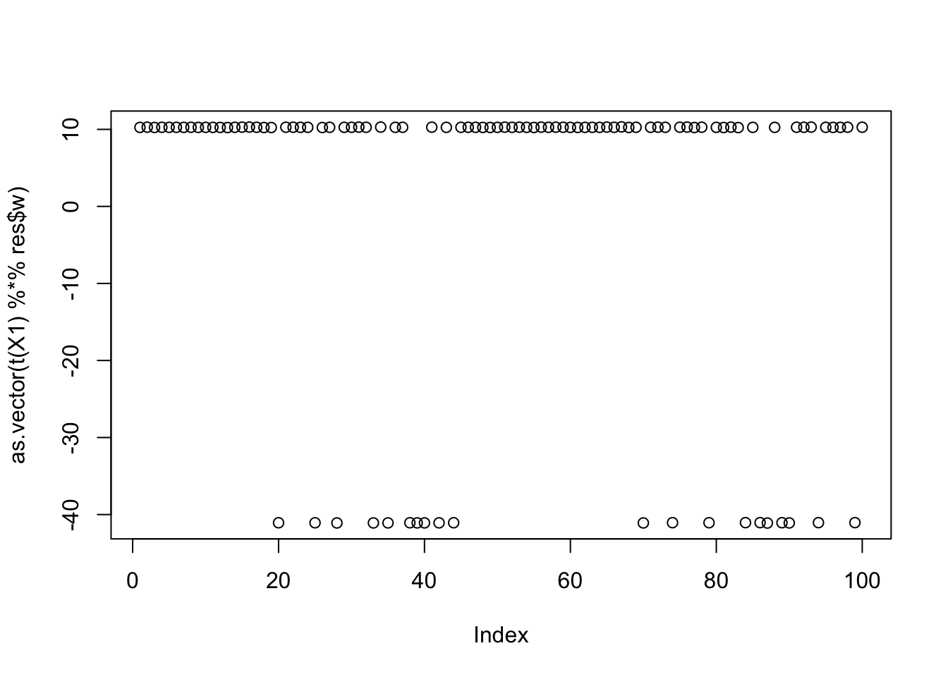
Here is the seed for the 11th biggest objective (finds the second factor)
seed= order(obj,decreasing=TRUE)[11]
set.seed(seed)
res = list(w = rnorm(nrow(X1)), c=0)
for(i in 1:100)
  res = fastica_r1update_wc(X1,res$w,res$c)
cor(L,t(X1) %*% res$w)
[,1]
[1,] 0.04258654
[2,] -0.11148268
[3,] -0.10750148plot(as.vector(t(X1) %*% res$w))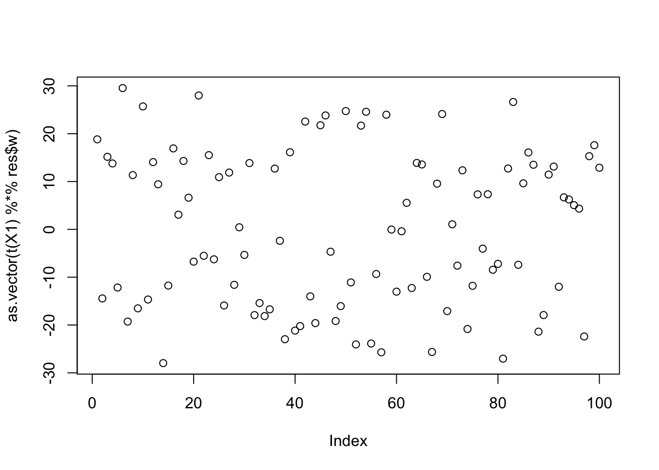
centered fastICA (PC starts)
We would probably like to find better ways to initialize so that we can find all the three solutions with fewer starts. I thought maybe it could be helpful to initialize from the PCs (ie w = (1,0,0..0) etc). There are 10 of these because I’m whitening to 10 dimensions. The first two PCs do indeed both find a group, and a different group for each one. This is promising - it suggests maybe we can get good starting points using the top PCs.
obj = rep(0,10)
for(pc in 1:10){
  w = rep(0,10)
  w[pc] = 1
  res = list(w = w, c=0)
  for(i in 1:100)
    res = fastica_r1update_wc(X1,res$w,res$c)
  obj[pc] = compute_objective(X1,res$w,res$c)
}
plot(obj)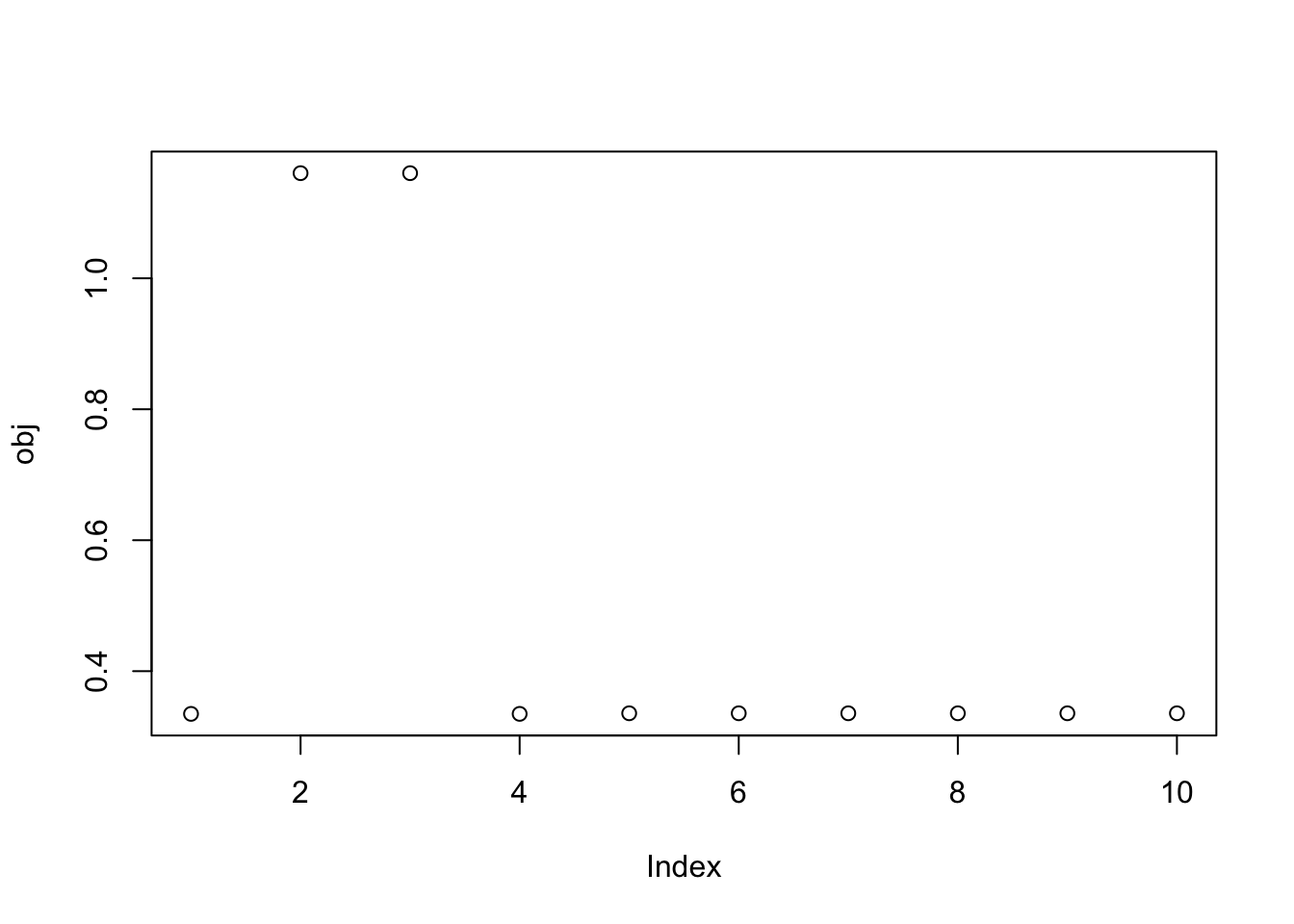
| Version | Author | Date |
|---|---|---|
| 7afc85f | Matthew Stephens | 2025-11-16 |
print(sort(obj,decreasing=TRUE)[1:10],digits=20) [1] 1.16052891191772578061 1.16052833896032780991 0.33569309204304309535
[4] 0.33569236181006040232 0.33569236180855116514 0.33569236180844630457
[7] 0.33569236180806799608 0.33569236180661360391 0.33479965888634471982
[10] 0.33478918679229641153Here I try random starts, but only weighting the top 3 PCs (which should be the ones with the signals). This successfully enriches for finding a good solution. It is a bit hard to see but these random starts do find all 3 of the different factors.
obj = rep(0,100)
for(seed in 1:100){
  set.seed(seed)
  res = list(w = c(rnorm(3),rep(0,7)), c=0)
  for(i in 1:100)
    res = fastica_r1update_wc(X1,res$w,res$c)
  obj[seed] = compute_objective(X1,res$w,res$c)
}
plot(log(max(obj)-obj))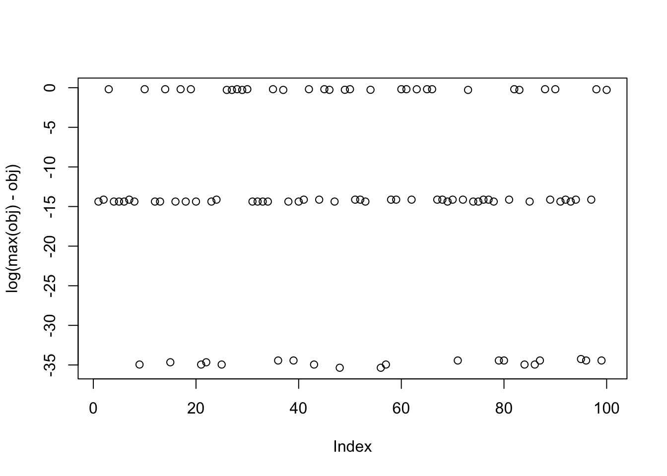
| Version | Author | Date |
|---|---|---|
| 7afc85f | Matthew Stephens | 2025-11-16 |
print(sort(obj-max(obj),decreasing=TRUE),digits=20) [1] 0.0000000000000000000e+00 0.0000000000000000000e+00
[3] 0.0000000000000000000e+00 -4.4408920985006261617e-16
[5] -4.4408920985006261617e-16 -6.6613381477509392425e-16
[7] -6.6613381477509392425e-16 -6.6613381477509392425e-16
[9] -6.6613381477509392425e-16 -6.6613381477509392425e-16
[11] -6.6613381477509392425e-16 -6.6613381477509392425e-16
[13] -8.8817841970012523234e-16 -8.8817841970012523234e-16
[15] -1.1102230246251565404e-15 -1.1102230246251565404e-15
[17] -1.1102230246251565404e-15 -1.1102230246251565404e-15
[19] -1.1102230246251565404e-15 -1.1102230246251565404e-15
[21] -1.1102230246251565404e-15 -1.1102230246251565404e-15
[23] -1.3322676295501878485e-15 -5.7295739863683081694e-07
[25] -5.7295739863683081694e-07 -5.7295739863683081694e-07
[27] -5.7295739863683081694e-07 -5.7295739908092002679e-07
[29] -5.7295739930296463172e-07 -5.7295739930296463172e-07
[31] -5.7295739930296463172e-07 -5.7295739930296463172e-07
[33] -5.7295739930296463172e-07 -5.7295739930296463172e-07
[35] -5.7295739930296463172e-07 -5.7295739952500923664e-07
[37] -5.7295739952500923664e-07 -5.7295739952500923664e-07
[39] -5.7295739952500923664e-07 -5.7295739952500923664e-07
[41] -5.7295739952500923664e-07 -5.7295739952500923664e-07
[43] -5.7295739952500923664e-07 -5.7295739952500923664e-07
[45] -5.7295739974705384157e-07 -5.7295739974705384157e-07
[47] -5.7295739974705384157e-07 -5.7295739974705384157e-07
[49] -5.7295739996909844649e-07 -7.2938177386738800578e-07
[51] -7.2938177408943261071e-07 -7.2938177408943261071e-07
[53] -7.2938177408943261071e-07 -7.2938177431147721563e-07
[55] -7.2938177431147721563e-07 -7.2938177431147721563e-07
[57] -7.2938177431147721563e-07 -7.2938177431147721563e-07
[59] -7.2938177431147721563e-07 -7.2938177431147721563e-07
[61] -7.2938177453352182056e-07 -7.2938177453352182056e-07
[63] -7.2938177453352182056e-07 -7.2938177453352182056e-07
[65] -7.2938177453352182056e-07 -7.2938177475556642548e-07
[67] -7.2938177475556642548e-07 -7.2938177475556642548e-07
[69] -7.2938177475556642548e-07 -7.2938177497761103041e-07
[71] -7.5641382430351467026e-01 -7.5641930268669210768e-01
[73] -7.5701004594153054050e-01 -7.5701004600101584607e-01
[75] -7.5701004984525943620e-01 -7.5765238076761654007e-01
[77] -7.5888592804964782879e-01 -7.6483359217003621389e-01
[79] -7.6754568945918366651e-01 -7.6802334733171306880e-01
[81] -8.1911547324708500195e-01 -8.1911547327230171955e-01
[83] -8.2480729140233477459e-01 -8.2483523861430496638e-01
[85] -8.2483586062517444404e-01 -8.2483652447530753093e-01
[87] -8.2483654468173117635e-01 -8.2483654787839433276e-01
[89] -8.2483654806860839948e-01 -8.2483654950253981752e-01
[91] -8.2483655010470391389e-01 -8.2483655011049950012e-01
[93] -8.2483655011380496713e-01 -8.2567807766327172558e-01
[95] -8.2571756401397278236e-01 -8.2572693829891297135e-01
[97] -8.2574645378866295964e-01 -8.2586640225611351873e-01
[99] -8.2598187574810000289e-01 -8.2653432775865576243e-019 groups
Now I try 9 groups, with 20 members each, which should be harder.
K=9
p = 1000
n = 100
set.seed(1)
L = matrix(0,nrow=n,ncol=K)
for(i in 1:K){L[sample(1:n,20),i]=1}
FF = matrix(rnorm(p*K), nrow = p, ncol=K)

X = L %*% t(FF) + rnorm(n*p,0,0.01)
plot(X %*% FF[,1])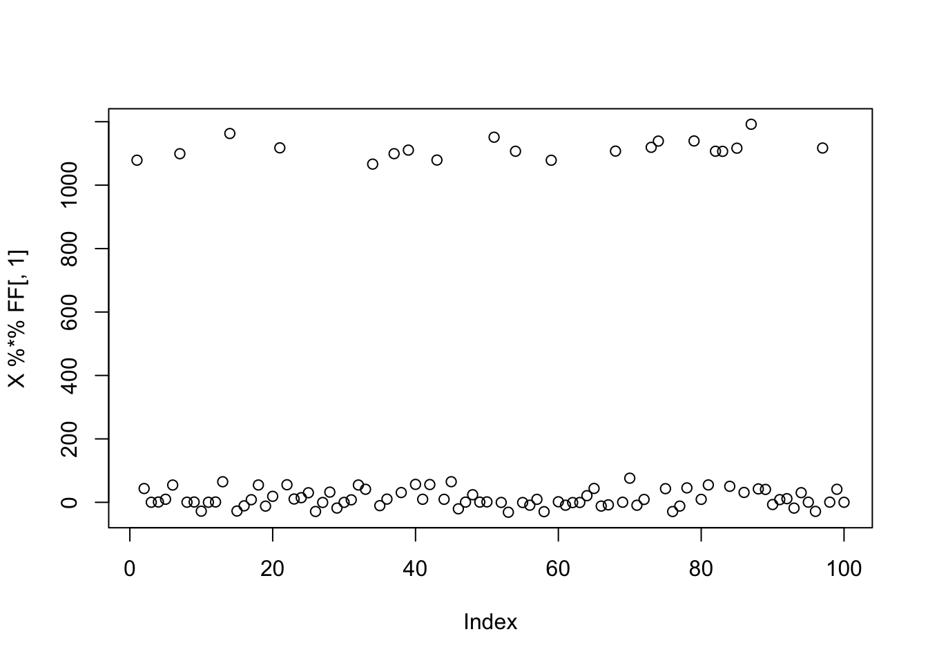
| Version | Author | Date |
|---|---|---|
| 7afc85f | Matthew Stephens | 2025-11-16 |
centered fastICA (random start)
As expected from above, initialization to a random w does not pick out a single source:
X1 = preprocess(X)
w = rnorm(nrow(X1))
c = 0 # this does not matter as c is updated first
res = list(w=w,c=c)
for(i in 1:100)
  res = fastica_r1update_wc(X1,res$w,res$c)
cor(L,t(X1) %*% res$w)
[,1]
[1,] -0.09726728
[2,] 0.30070236
[3,] 0.13628099
[4,] 0.48908080
[5,] 0.11271536
[6,] 0.30924678
[7,] 0.42893419
[8,] 0.55328213
[9,] -0.02730030plot(as.vector(t(X1) %*% res$w))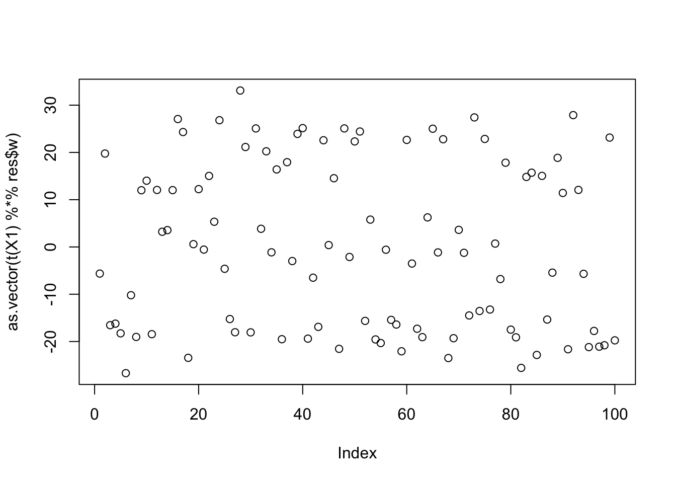
| Version | Author | Date |
|---|---|---|
| 7afc85f | Matthew Stephens | 2025-11-16 |
res$c[1] 0.03743987compute_objective(X1,res$w,res$c)[1] 0.4095468centered fastICA (true factor start)
Now I try initializing at (or close to) a true factor: again it converges to the solution I wanted, and has a much higher objective than then random start.
w = X1 %*% L[,1]
plot(t(X1) %*% w)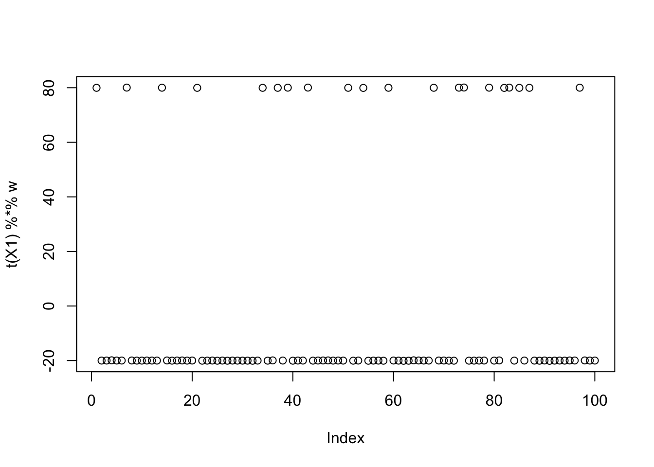
| Version | Author | Date |
|---|---|---|
| 7afc85f | Matthew Stephens | 2025-11-16 |
c = 0 # note this does not matter much because c gets updated first in the algorithm
res = list(w=w,c=c)
print(compute_objective(X1,res$w,res$c), digits=20)
[1] 0.36109216320642395504for(i in 1:100)
res = fastica_r1update_wc(X1,res$w,res$c)
cor(L,t(X1) %*% res$w) [,1]
[1,] 9.999996e-01
[2,] 1.243654e-04
[3,] -6.253190e-02
[4,] 1.551905e-05
[5,] 6.251122e-02
[6,] -3.316446e-05
[7,] -6.251458e-02
[8,] 6.260251e-02
[9,] -6.256465e-02plot(as.vector(t(X1) %*% res$w))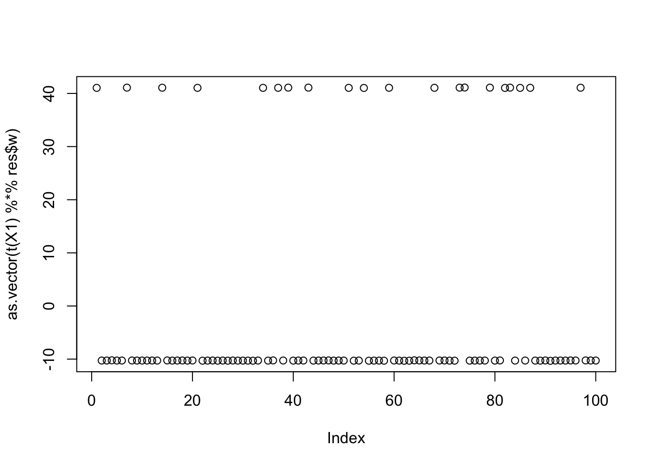
print(compute_objective(X1,res$w,res$c), digits=20)[1] 1.1605285638478726185centered fastICA (many random starts)
Here I try with 100 random starts - there are lots of different results, and some of them reach objectives similar to that from the true starts.
obj = rep(0,100)
for(seed in 1:100){
set.seed(seed)
res = list(w = rnorm(nrow(X1)), c=0)
for(i in 1:100)
res = fastica_r1update_wc(X1,res$w,res$c)
obj[seed] = compute_objective(X1,res$w,res$c)
}
plot(obj)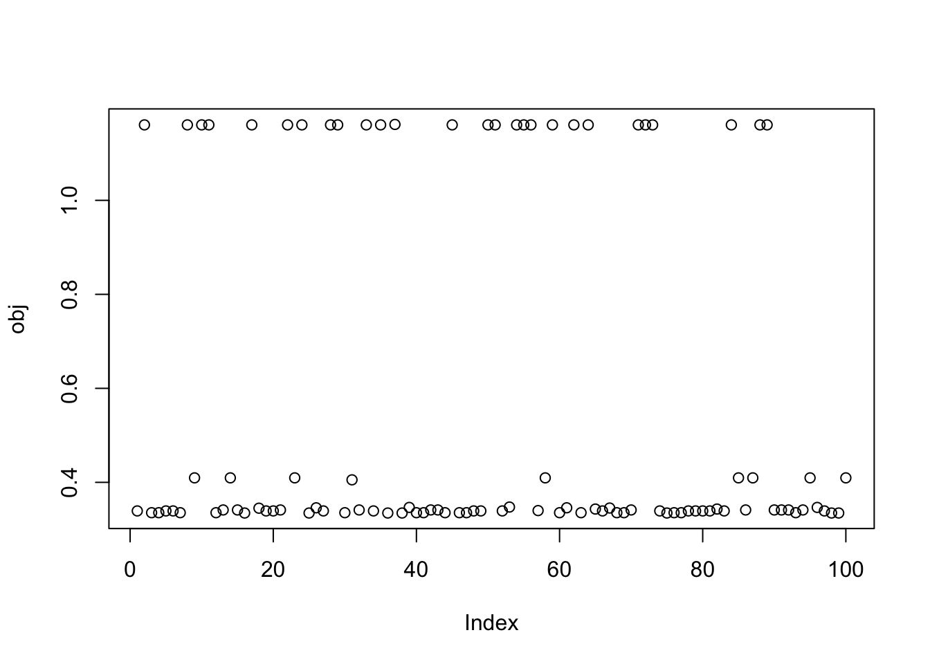
| Version | Author | Date |
|---|---|---|
| 7afc85f | Matthew Stephens | 2025-11-16 |
print(sort(obj,decreasing=TRUE)[1:20],digits=20) [1] 1.1614533280555634498 1.1605284588712569960 1.1605284588712567739
[4] 1.1605283085989401837 1.1605283085989401837 1.1605283085989397396
[7] 1.1605282664300622386 1.1605282663666407483 1.1605282663666405263
[10] 1.1605282663666400822 1.1605282663666400822 1.1605282663666400822
[13] 1.1605282226977386983 1.1605282226977384763 1.1605282226977380322
[16] 1.1605281785009746720 1.1605281785009744500 1.1605281374473852551
[19] 1.1605281374473850331 1.1605281374473845890This is the top seed - finds group 9
seed= order(obj,decreasing=TRUE)[1]
set.seed(seed)
res = list(w = rnorm(nrow(X1)), c=0)
for(i in 1:100)
  res = fastica_r1update_wc(X1,res$w,res$c)
cor(L,t(X1) %*% res$w)
[,1]
[1,] -0.06252853
[2,] -0.06257660
[3,] -0.25000013
[4,] 0.06255022
[5,] -0.06239568
[6,] 0.06260440
[7,] -0.06246353
[8,] -0.12503198
[9,] 0.99999964plot(as.vector(t(X1) %*% res$w))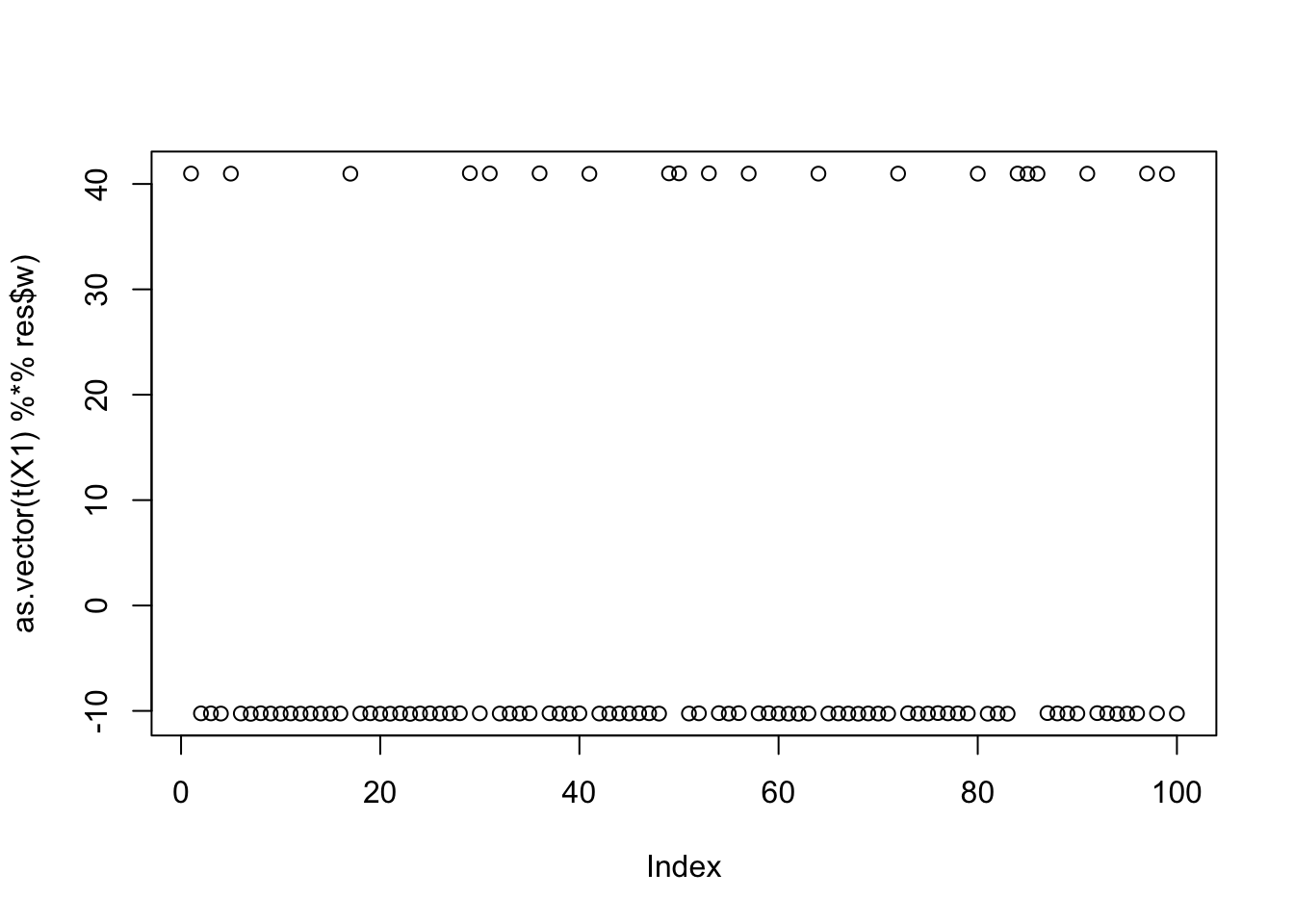
| Version | Author | Date |
|---|---|---|
| 7afc85f | Matthew Stephens | 2025-11-16 |
max(obj)[1] 1.161453Here is the seed for the 2nd biggest objective (finds the 6th factor)
seed= order(obj,decreasing=TRUE)[2]
set.seed(seed)
res = list(w = rnorm(nrow(X1)), c=0)
for(i in 1:100)
res = fastica_r1update_wc(X1,res$w,res$c)
cor(L,t(X1) %*% res$w) [,1]
[1,] -1.660329e-04
[2,] 6.260188e-02
[3,] 1.037251e-05
[4,] 6.251477e-02
[5,] -6.248630e-02
[6,] 9.999997e-01
[7,] -6.258321e-02
[8,] -6.251282e-02
[9,] 6.251728e-02plot(as.vector(t(X1) %*% res$w))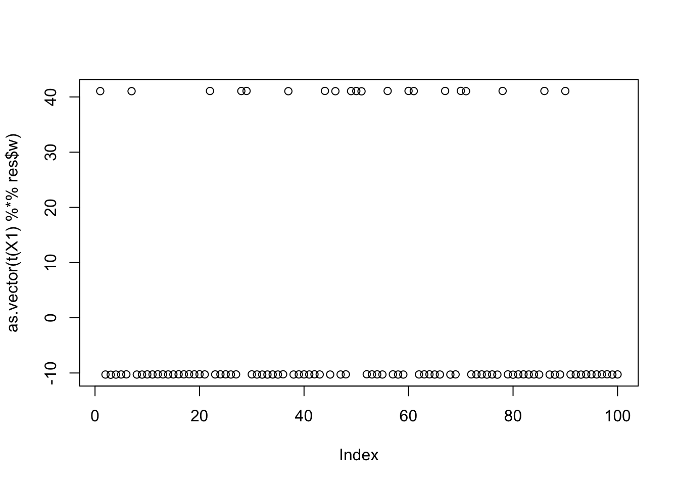
Here is the seed for the 4rd biggest objective (finds factor 5)
seed= order(obj,decreasing=TRUE)[4]
set.seed(seed)
res = list(w = rnorm(nrow(X1)), c=0)
for(i in 1:100)
res = fastica_r1update_wc(X1,res$w,res$c)
cor(L,t(X1) %*% res$w) [,1]
[1,] 0.0625264460
[2,] 0.0624722551
[3,] -0.0000935853
[4,] -0.0625035238
[5,] 0.9999996548
[6,] -0.0625365535
[7,] 0.0624249370
[8,] 0.0623628638
[9,] -0.0625123794plot(as.vector(t(X1) %*% res$w))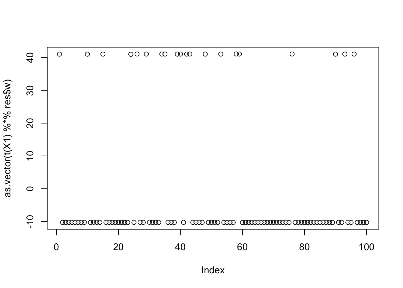
| Version | Author | Date |
|---|---|---|
| 7afc85f | Matthew Stephens | 2025-11-16 |
Try finding two groups
It turns out that factors 3 and 9 are not overlapping in this simulation, so I wondered whether combining them would be a good solution. Initializing at that combination does find the combined solution, but the objective is lower than for a single group because the objective favors unbalanced groups.
w = X1 %*% (L[,3] + L[,9])
plot(t(X1) %*% w)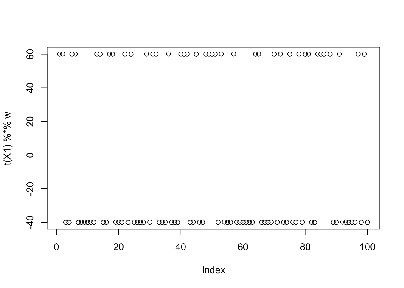
| Version | Author | Date |
|---|---|---|
| 7afc85f | Matthew Stephens | 2025-11-16 |
c = 0 # note this does not matter much because c gets updated first in the algorithm
res = list(w=w,c=c)
print(compute_objective(X1,res$w,res$c), digits=20)[1] 0.42683383934382418401for(i in 1:100)
res = fastica_r1update_wc(X1,res$w,res$c)
cor(L,t(X1) %*% res$w) [,1]
[1,] -0.10209493
[2,] -0.05104159
[3,] 0.61284517
[4,] 0.10209644
[5,] -0.05104948
[6,] 0.05101982
[7,] 0.10212606
[8,] 0.05127832
[9,] 0.61189897plot(as.vector(t(X1) %*% res$w))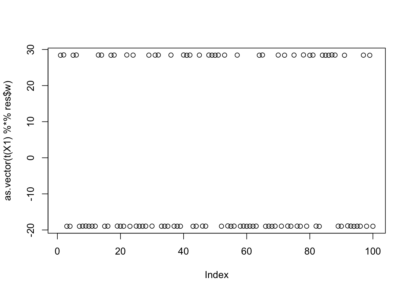
print(compute_objective(X1,res$w,res$c), digits=20)[1] 0.42186249079217386093Interestingly this seems to be an unstable solution: if I initialize nearby then it moves away to a single group.
w = X1 %*% (0.45*L[,3] + 0.55*L[,9])
plot(t(X1) %*% w)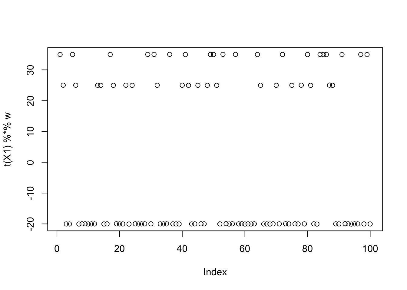
| Version | Author | Date |
|---|---|---|
| 7afc85f | Matthew Stephens | 2025-11-16 |
c = 0 # note this does not matter much because c gets updated first in the algorithm
res = list(w=w,c=c)
print(compute_objective(X1,res$w,res$c), digits=20)[1] 0.4231997098956051806for(i in 1:100)
res = fastica_r1update_wc(X1,res$w,res$c)
cor(L,t(X1) %*% res$w) [,1]
[1,] 6.251420e-02
[2,] -1.862304e-05
[3,] -9.999997e-01
[4,] -6.252398e-02
[5,] 2.902059e-05
[6,] -7.230353e-05
[7,] -1.874381e-01
[8,] -1.874072e-01
[9,] 2.500002e-01plot(as.vector(t(X1) %*% res$w))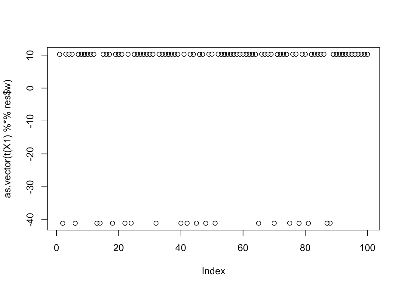
print(compute_objective(X1,res$w,res$c), digits=20)[1] 1.1605280894817924242Four non-overlapping groups
Here I look at 4 equal non-overlapping groups. I’m interested in whether it converges to a single group or a combination of groups, and whether the combination of 2 groups is a stable or unstable solution. It turns out that the vast majority of random starts converge to a combination of 2 groups, which is very different behavior than above. It gets me wondering whether this is because i) the non-overlapping situation, or ii) the symmetry created by the fact there are only 4 groups (2 vs 2).
set.seed(1)
n = 100
p = 1000
L = matrix(0,nrow=n,ncol=4)
L[1:25,1] = 1
L[26:50,2] = 1
L[51:75,3] = 1
L[76:100,4] = 1
FF = matrix(rnorm(p*4),nrow=p)
X = L %*% t(FF) + rnorm(n*p,0,0.01)
image(X%*% t(X))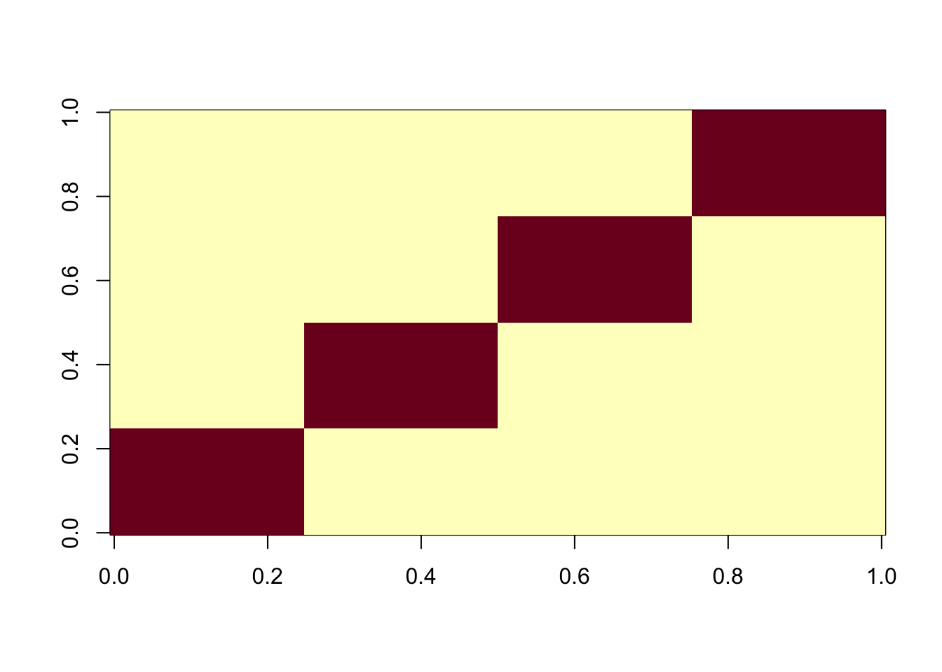
X1 = preprocess(X,n.comp=4)centered fastICA (many random starts)
Here I try with 100 random starts. Two seeds find a big objective (turns out to correspond to a single group) and others find what looks like a very similar objective (turns out to correspond to a combination of two groups).
obj = rep(0,100)
for(seed in 1:100){
  set.seed(seed)
  res = list(w = rnorm(nrow(X1)), c=0)
  for(i in 1:100)
    res = fastica_r1update_wc(X1,res$w,res$c)
  obj[seed] = compute_objective(X1,res$w,res$c)
}
plot(obj)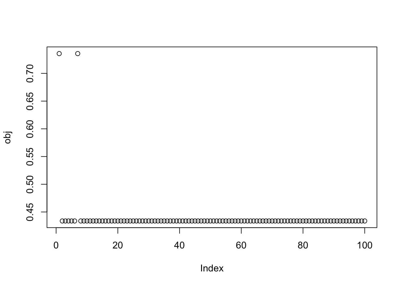
Here is the seed for the biggest objective (finds factor 3)
seed= order(obj,decreasing=TRUE)[1]
set.seed(seed)
res = list(w = rnorm(nrow(X1)), c=0)
for(i in 1:100)
  res = fastica_r1update_wc(X1,res$w,res$c)
cor(L,t(X1) %*% res$w)
[,1]
[1,] -0.3333332
[2,] -0.3333333
[3,] 0.9999998
[4,] -0.3333333plot(as.vector(t(X1) %*% res$w))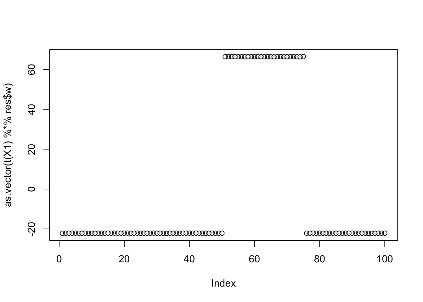
Here is the seed for the 2nd biggest objective (finds factor 2)
seed= order(obj,decreasing=TRUE)[2]
set.seed(seed)
res = list(w = rnorm(nrow(X1)), c=0)
for(i in 1:100)
  res = fastica_r1update_wc(X1,res$w,res$c)
cor(L,t(X1) %*% res$w)
[,1]
[1,] 0.3333333
[2,] -0.9999998
[3,] 0.3333333
[4,] 0.3333332plot(as.vector(t(X1) %*% res$w))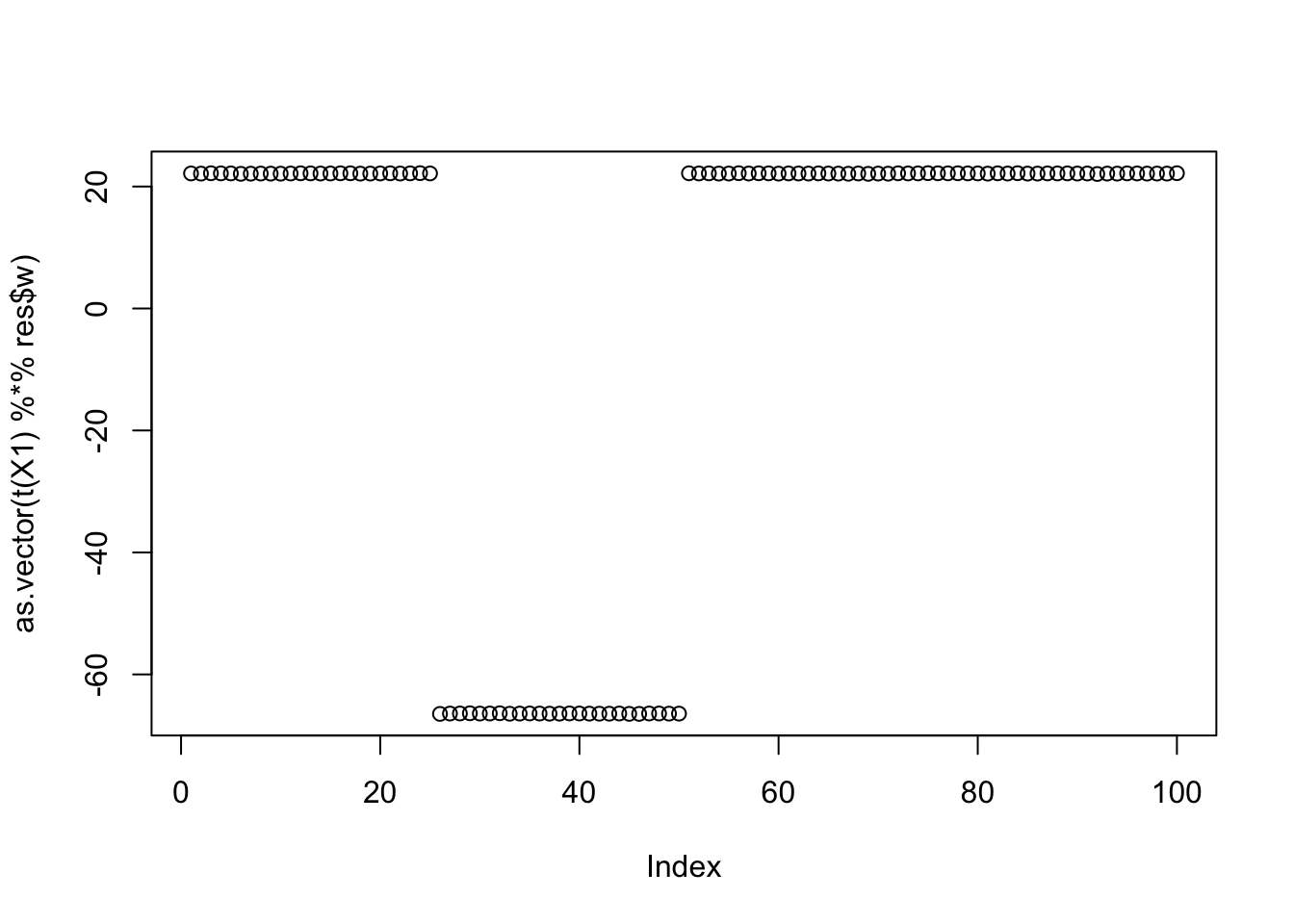
Here is the seed for the 3rd biggest objective (finds two combined factors)
seed= order(obj,decreasing=TRUE)[3]
set.seed(seed)
res = list(w = rnorm(nrow(X1)), c=0)
for(i in 1:100)
res = fastica_r1update_wc(X1,res$w,res$c)
cor(L,t(X1) %*% res$w) [,1]
[1,] -0.5773502
[2,] 0.5773502
[3,] 0.5773501
[4,] -0.5773501plot(as.vector(t(X1) %*% res$w))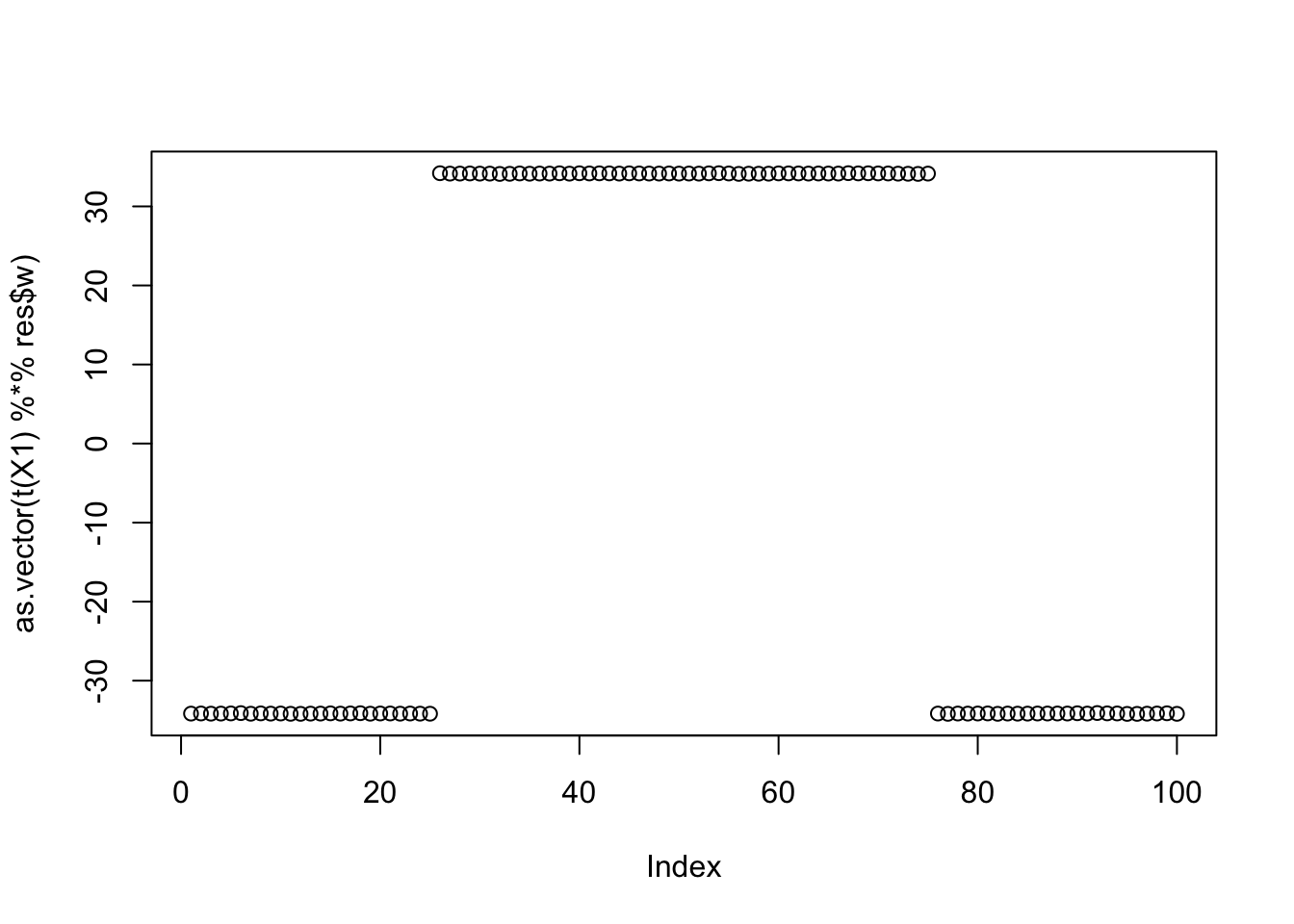
Nine non-overlapping groups
Here I look at 9 equal non-overlapping groups.
Start by creating L to be a binary matrix with 9 columns, 25*9 rows, and a single 1 in each row.
set.seed(1)
n = 225
p = 1000
L = matrix(0,nrow=n,ncol=9)
for(i in 1:9){L[((i-1)*25+1):(i*25),i] = 1}
FF = matrix(rnorm(p*9),nrow=p)
X = L %*% t(FF) + rnorm(n*p,0,0.01)
image(X%*% t(X))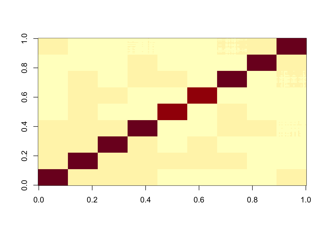
X1 = preprocess(X,n.comp=10)centered fastICA (many random starts)
Here I try with 100 random starts - it turns out that the objective goes off to infinity a lot, with c getting very large. This was unexpected, but maybe with hindsight the surprising thing is that we did not see the behaviour previously! The objective is indeed unbounded as we let c go to infinity. I think that intuitively this is equivalent to putting all the points in a single group. We need to do something to avoid this - maybe constrain c so that the values of Xw+c span both sides of 0. So max(Xw)+c > 0 and min(Xw) + c < 0. Or equivalently -max(Xw)< c < -min(Xw).
obj = rep(0,100)
for(seed in 1:100){
set.seed(seed)
res = list(w = rnorm(nrow(X1)), c=0)
for(i in 1:100)
res = fastica_r1update_wc(X1,res$w,res$c)
obj[seed] = compute_objective(X1,res$w,res$c)
}
plot(obj)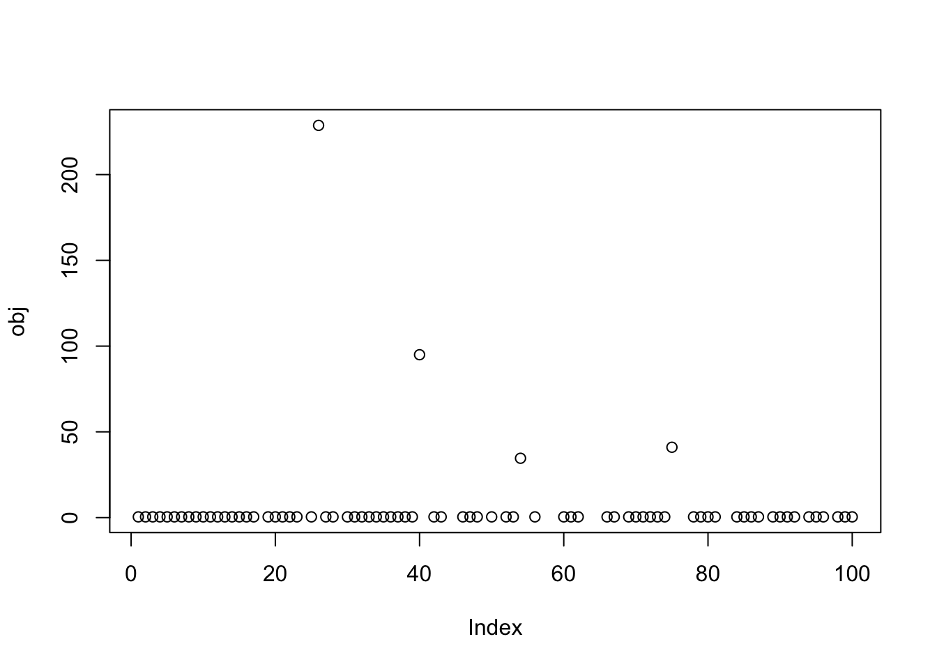
obj [1] 0.4300068 0.4300067 0.4300068 0.4300068 0.4300067 0.4300068
[7] 0.4300068 0.4300068 0.4300068 0.4300068 0.4300068 0.4300068
[13] 0.4300068 0.4300068 0.4300068 0.4300068 0.4300068 Inf
[19] 0.4300068 0.4300068 0.4300068 0.4300068 0.4300068 Inf
[25] 0.4300068 228.6990605 0.4300068 0.4300068 Inf 0.4300068
[31] 0.4300068 0.4300068 0.4300068 0.4300068 0.4300067 0.4300068
[37] 0.4300068 0.4300067 0.4300068 94.9776736 Inf 0.4300068
[43] 0.4300068 Inf Inf 0.4300067 0.4300068 0.4300068
[49] Inf 0.4300068 Inf 0.4300068 0.4300068 34.5982027
[55] Inf 0.4300068 Inf Inf Inf 0.4300068
[61] 0.4300068 0.4300068 Inf Inf Inf 0.4300068
[67] 0.4300068 Inf 0.4300068 0.4300068 0.4300068 0.4300068
[73] 0.4300068 0.4300068 41.0272630 Inf Inf 0.4300068
[79] 0.4300068 0.4300068 0.4300068 Inf Inf 0.4300068
[85] 0.4300068 0.4300068 0.4300068 Inf 0.4300068 0.4300068
[91] 0.4300068 0.4300068 Inf 0.4300067 0.4300068 0.4300068
[97] Inf 0.4300068 0.4300068 0.4300068res$c[1] 0.08702684Here are some results for non-infinite objectives: they find solutions corresponding to a split of the data into two groups.
seed= 1
set.seed(seed)
res = list(w = rnorm(nrow(X1)), c=0)
for(i in 1:100)
res = fastica_r1update_wc(X1,res$w,res$c)
cor(L,t(X1) %*% res$w) [,1]
[1,] -0.3952846
[2,] 0.3162276
[3,] -0.3952845
[4,] 0.3162278
[5,] 0.3162278
[6,] 0.3162278
[7,] -0.3952846
[8,] 0.3162273
[9,] -0.3952846plot(as.vector(t(X1) %*% res$w))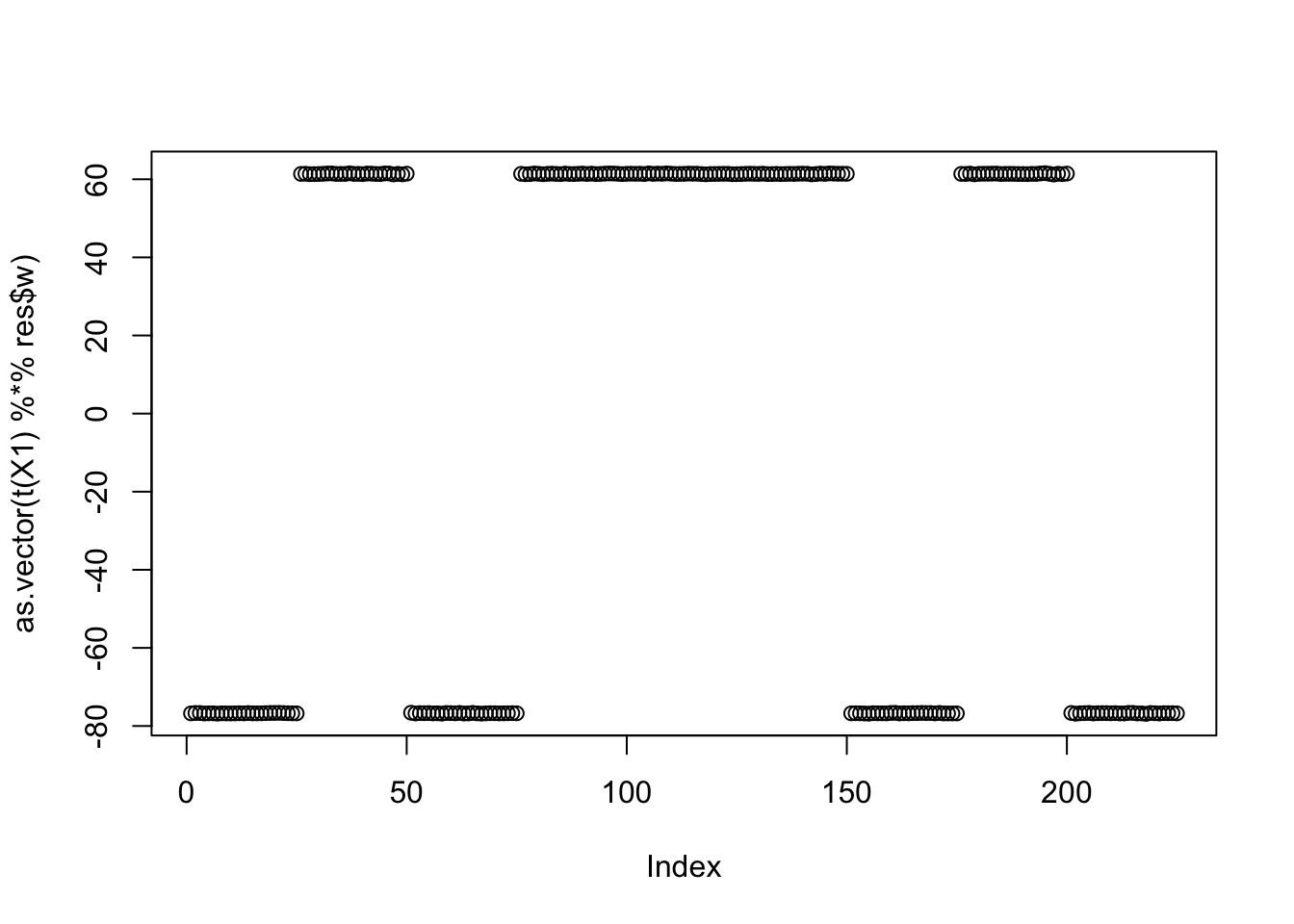
res$c[1] -0.08702687seed= 2
set.seed(seed)
res = list(w = rnorm(nrow(X1)), c=0)
for(i in 1:100)
res = fastica_r1update_wc(X1,res$w,res$c)
cor(L,t(X1) %*% res$w) [,1]
[1,] 0.3162278
[2,] -0.3952847
[3,] -0.3952844
[4,] -0.3952845
[5,] 0.3162276
[6,] 0.3162274
[7,] -0.3952845
[8,] 0.3162278
[9,] 0.3162276plot(as.vector(t(X1) %*% res$w))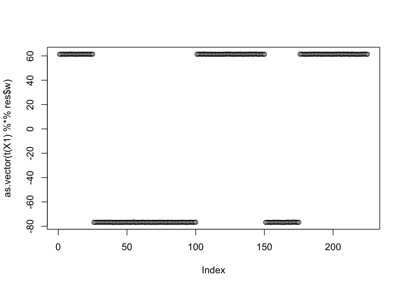
res$c[1] -0.087027Here I try initializing at a single group: I find the solution goes off to c=infinity.
w = X1 %*% L[,1]
plot(t(X1) %*% w)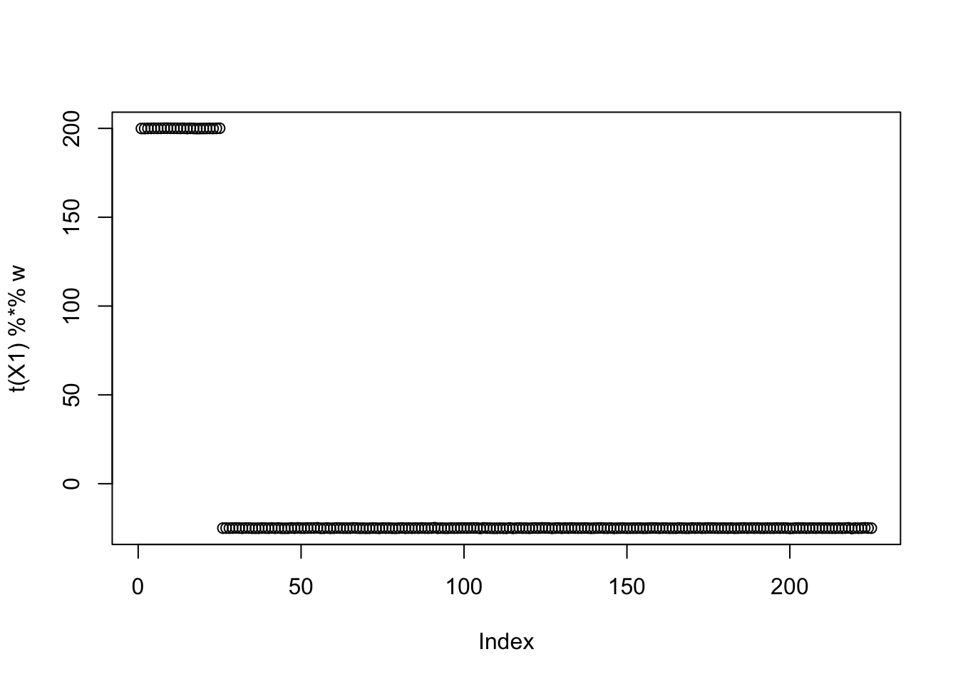
c = 0 # note this does not matter much because c gets updated first in the algorithm
res = list(w=w,c=c)
print(compute_objective(X1,res$w,res$c), digits=20)
[1] 0.2920762940026140897for(i in 1:100)
res = fastica_r1update_wc(X1,res$w,res$c)
cor(L,t(X1) %*% res$w) [,1]
[1,] 5.123949e-03
[2,] 4.897611e-03
[3,] -1.774167e-02
[4,] -8.640341e-05
[5,] -2.313242e-03
[6,] 6.944872e-03
[7,] -1.625867e-02
[8,] 1.497577e-03
[9,] 1.793597e-02plot(as.vector(t(X1) %*% res$w))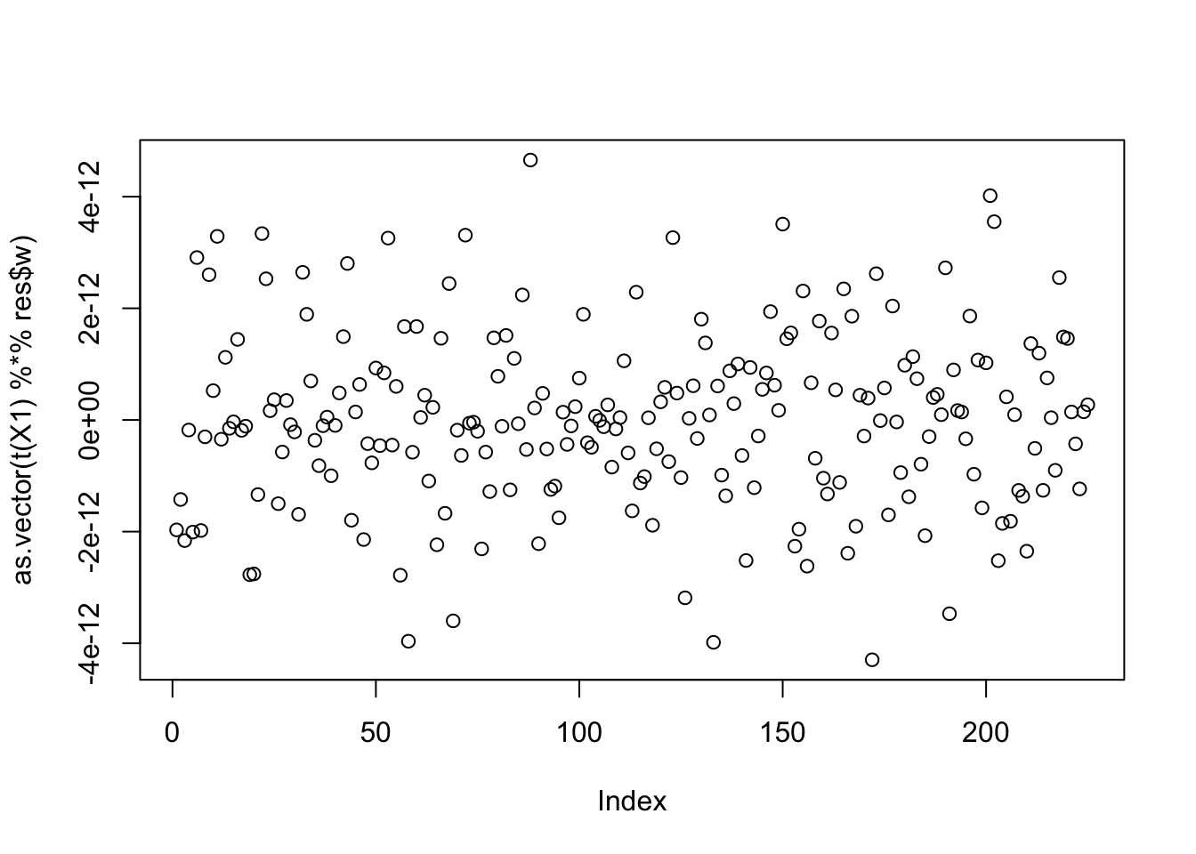
print(compute_objective(X1,res$w,res$c), digits=20)[1] InfTree simulations
Here is a simple tree-based simulations; it’s a 4-leaf tree with two bifurcating branches.
# set up L to be a tree with 4 tips and 7 branches (including top shared branch)
set.seed(1)
n = 100
p = 1000
L = matrix(0,nrow=n,ncol=6)
L[1:50,1] = 1 #top split L
L[51:100,2] = 1 # top split R
L[1:25,3] = 1
L[26:50,4] = 1
L[51:75,5] = 1
L[76:100,6] = 1
FF = matrix(rnorm(p*6),nrow=p)
X = L %*% t(FF) + rnorm(n*p,0,0.01)
image(X%*% t(X))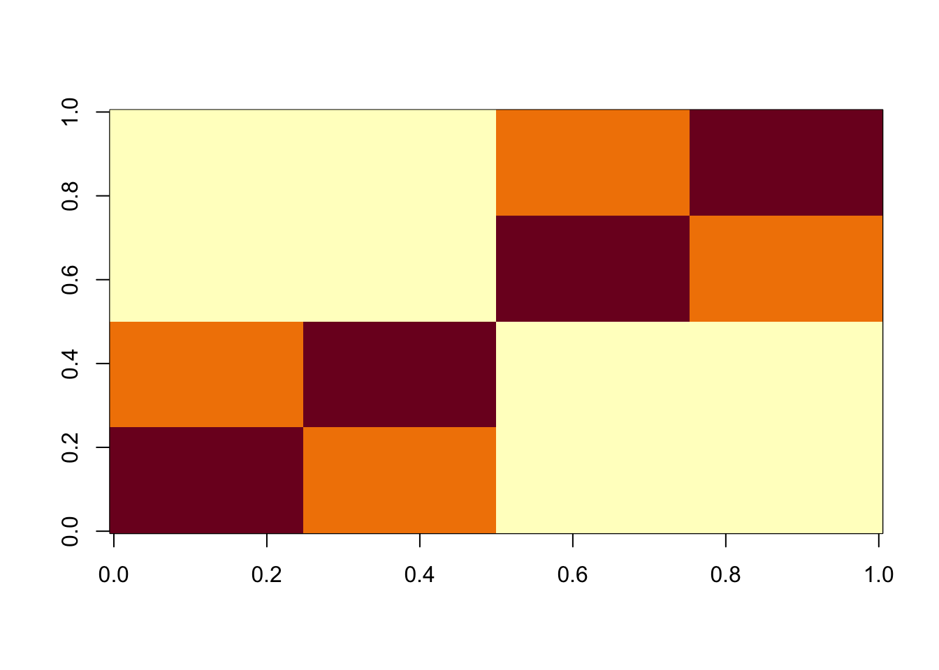
X1 = preprocess(X)Run 100 seeds, weighting only the top 3 PCs in the initialization (note: when I did the same weighting the top 4 PCs I got more mixed branch solutions). We see that the top seeds pick out a single group. Next seeds are the top branch, but then after that we have a bunch of seeds that combine two groups that are not adjacent on the tree - these solutions are less attractive to us. We need to find a way to find more of the single-branch solutions, and, ideally, avoid these mixed-branch solutions (although it might be possible to filter these somehow at the end). One thing I don’t quite understand is that the objective for the mixed branch solutions seems to be consistently, but very slightly, lower than for the single-branch solution. That would be good to understand better.
obj = rep(0,100)
Lhat = matrix(nrow=100,ncol=n)
for(seed in 1:100){
set.seed(seed)
res = list(w = c(rnorm(3),rep(0,7)), c=0)
for(i in 1:100)
res = fastica_r1update_wc(X1,res$w,res$c)
obj[seed] = compute_objective(X1,res$w,res$c)
Lhat[seed,] = t(X1) %*% res$w
}
plot(obj)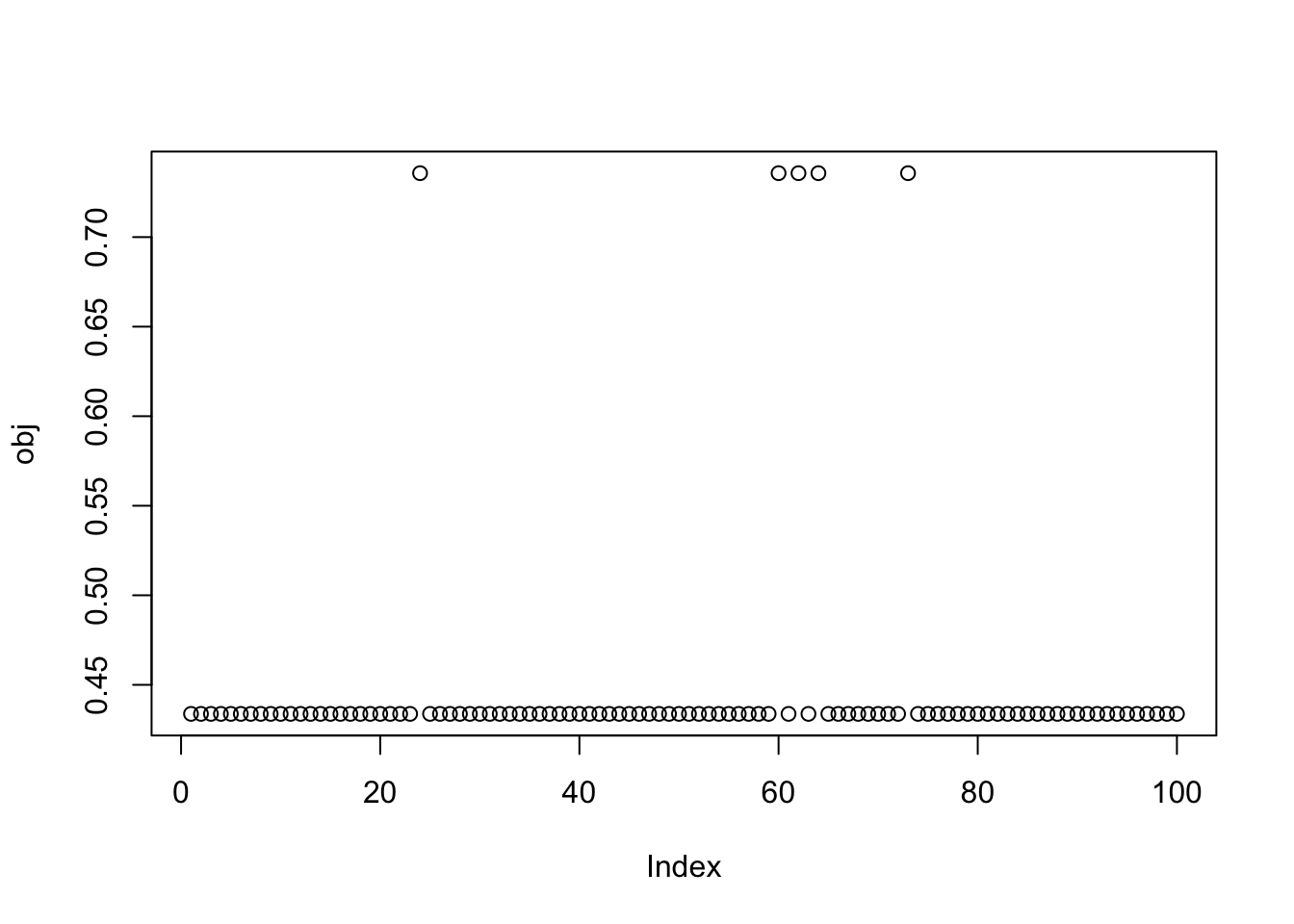
image(Lhat[order(obj,decreasing=TRUE),])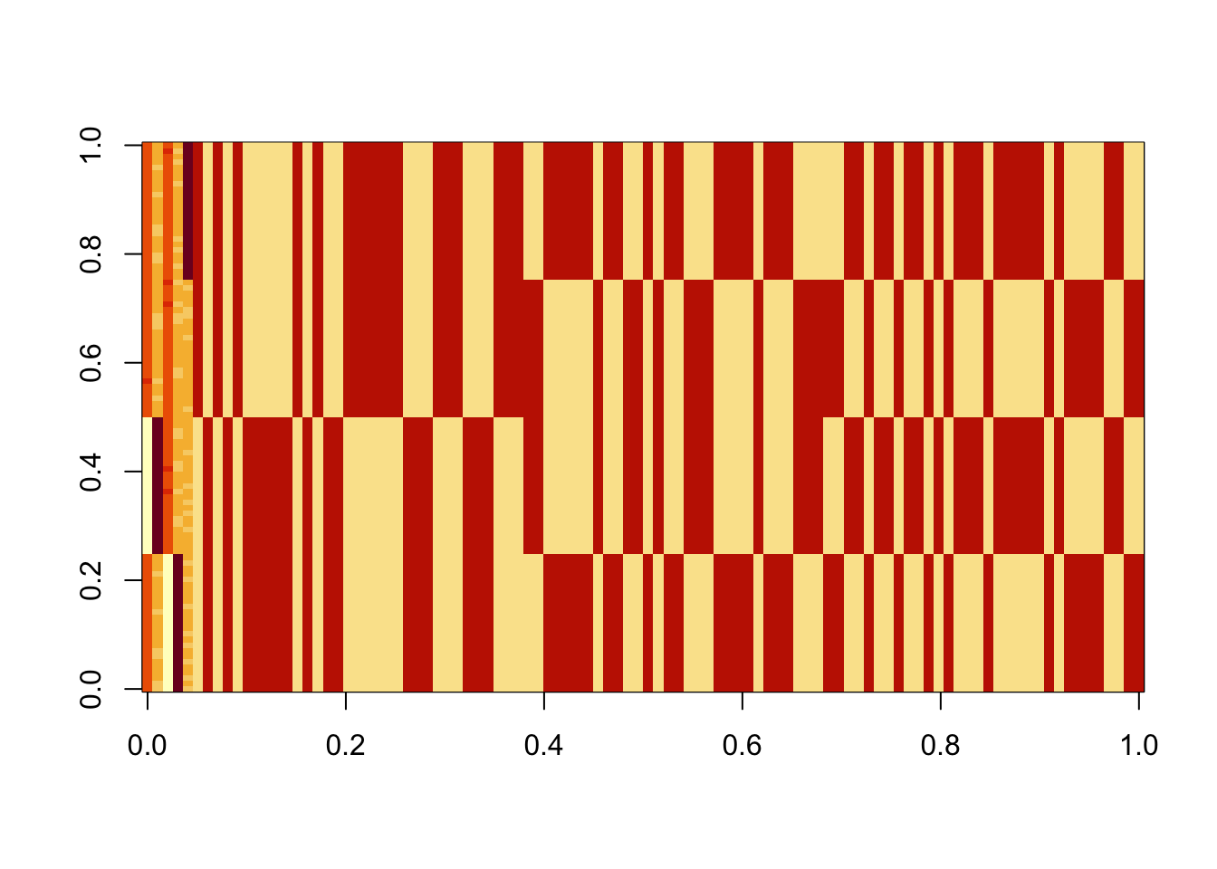
The top seed is a single group:
seed = order(obj,decreasing=TRUE)[1]
set.seed(seed)
res = list(w = c(rnorm(3),rep(0,7)), c=0)
for(i in 1:100)
  res = fastica_r1update_wc(X1,res$w,res$c)
cor(L,t(X1) %*% res$w)
[,1]
[1,] -0.5773503
[2,] 0.5773503
[3,] 0.3333332
[4,] -0.9999999
[5,] 0.3333333
[6,] 0.3333333plot(as.vector(t(X1) %*% res$w))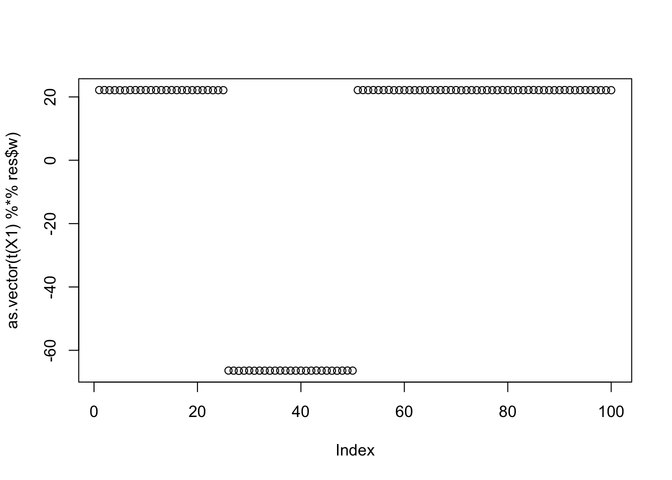
Results for the third biggest seed:
seed = order(obj,decreasing=TRUE)[3]
set.seed(seed)
res = list(w = c(rnorm(3),rep(0,7)), c=0)
for(i in 1:100)
  res = fastica_r1update_wc(X1,res$w,res$c)
cor(L,t(X1) %*% res$w)
[,1]
[1,] -0.5773502
[2,] 0.5773502
[3,] -0.9999999
[4,] 0.3333332
[5,] 0.3333334
[6,] 0.3333333plot(as.vector(t(X1) %*% res$w))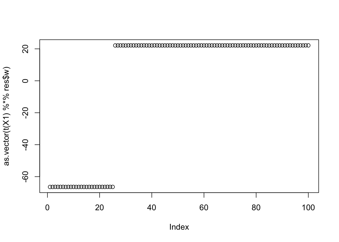
Noting here an idea to investigate: maybe initialize w “orthogonal” to previous ones (but don’t impose orthogonality during iterations) to try to find different solutions? Here’s what I mean. The problem is that there are 5 solutions we want to find here - not sure how to try to find all of them.
set.seed(1)
w.init = c(rnorm(3),rep(0,7))
w.init = w.init - sum(w.init * res$w)/(sum(res$w^2)) * res$w
res = list(w = w.init, c=0)
for(i in 1:100)
  res = fastica_r1update_wc(X1,res$w,res$c)
cor(L,t(X1) %*% res$w)
[,1]
[1,] 0.9999999
[2,] -0.9999999
[3,] 0.5773503
[4,] 0.5773502
[5,] -0.5773503
[6,] -0.5773502plot(as.vector(t(X1) %*% res$w))
Initialize in the original space
Here I try initializing by a random linear combination of the columns of the original X. Then I choose w so that X1’ w equals this l1.
set.seed(1)
w1 = rnorm(ncol(X)) # linear comb of columns in the original space
l1 = X %*% w1
w = X1 %*% l1
w.init = w/mean(w^2)
plot(t(X1) %*% w.init, l1)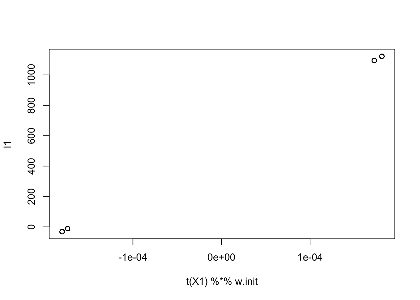
Initializing here gives the two groups.
res = list(w = w.init, c=0)
for(i in 1:100)
  res = fastica_r1update_wc(X1,res$w,res$c)
cor(L,t(X1) %*% res$w)
[,1]
[1,] 0.9999999
[2,] -0.9999999
[3,] 0.5773503
[4,] 0.5773502
[5,] -0.5773503
[6,] -0.5773502plot(as.vector(t(X1) %*% res$w))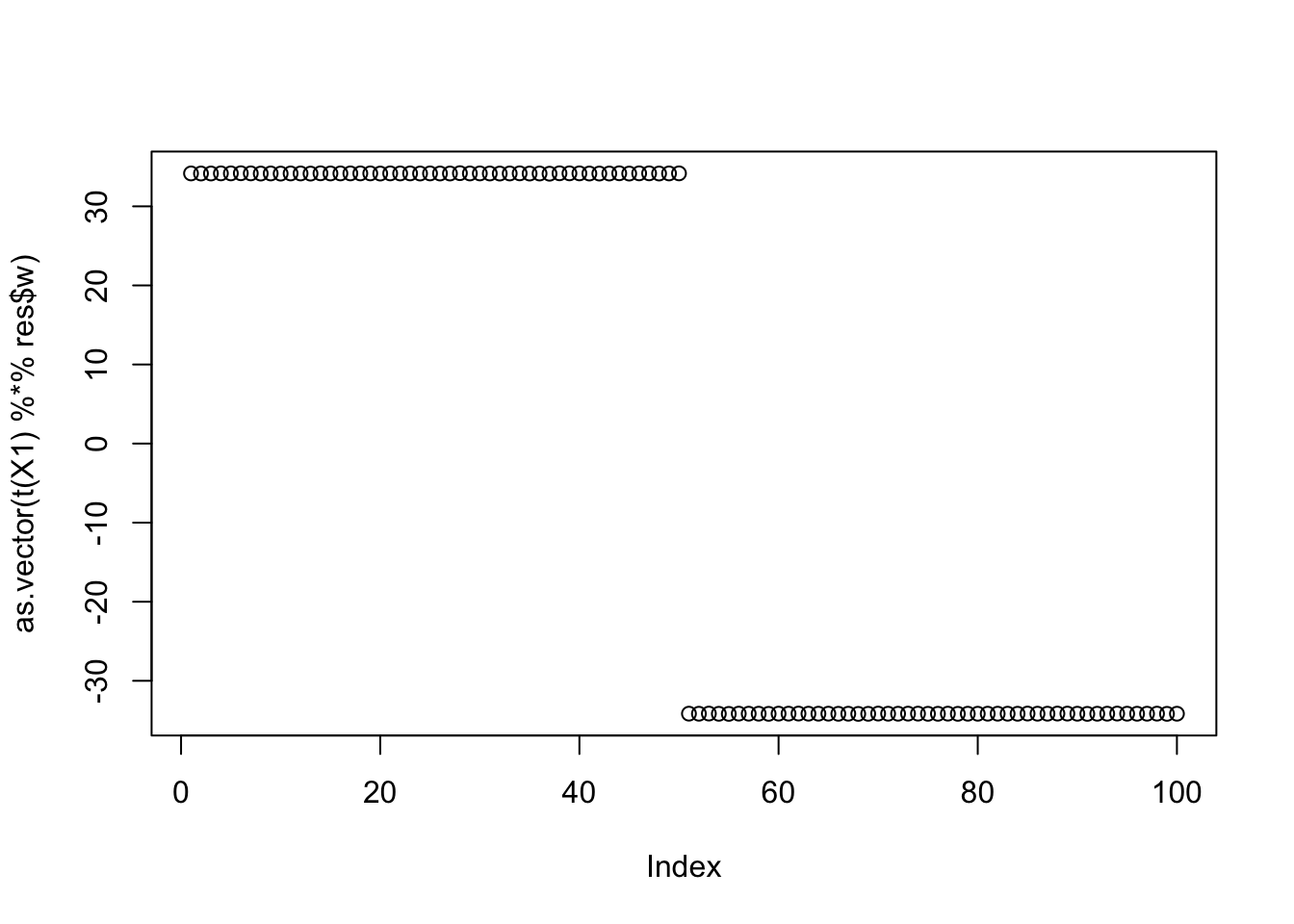
lhat = t(X1) %*% res$w
what = t(X) %*% lhat # finds an optimal w in the original space
Now find the what in the original space that corresponds to this solution, and initialize orthogonal to what in the original space
w1 = rnorm(ncol(X))
w1 = w1 - sum(w1 * what)/(sum(what^2)) * what # orthogonal to what

l1 = X %*% w1
w = X1 %*% l1
w.init = w/mean(w^2)
plot(t(X1) %*% w.init, l1)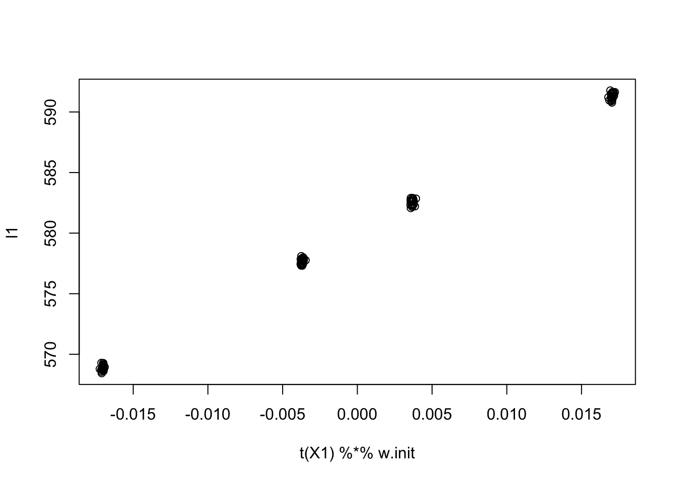
Running from this one produces a mixed group. And this seems to happen repeatedly with this strategy. Need to investigate this more carefully.
res = list(w = w.init, c=0)
for(i in 1:100)
  res = fastica_r1update_wc(X1,res$w,res$c)
cor(L,t(X1) %*% res$w)
[,1]
[1,] -8.913993e-09
[2,] 8.913993e-09
[3,] 5.773502e-01
[4,] -5.773502e-01
[5,] -5.773502e-01
[6,] 5.773502e-01plot(as.vector(t(X1) %*% res$w))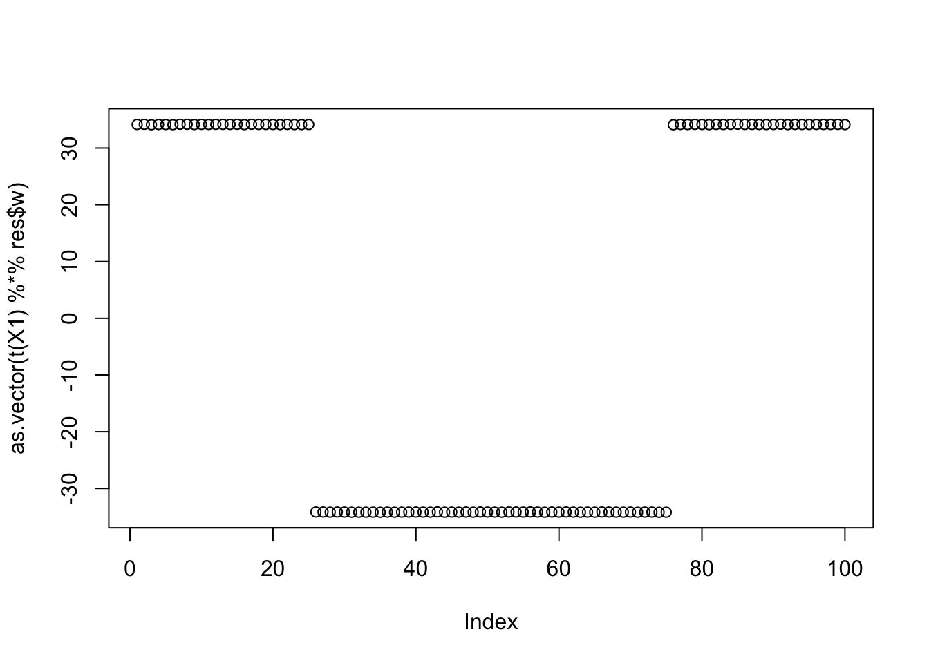
sessionInfo()R version 4.4.2 (2024-10-31)
Platform: aarch64-apple-darwin20
Running under: macOS Sequoia 15.6.1
Matrix products: default
BLAS: /Library/Frameworks/R.framework/Versions/4.4-arm64/Resources/lib/libRblas.0.dylib
LAPACK: /Library/Frameworks/R.framework/Versions/4.4-arm64/Resources/lib/libRlapack.dylib; LAPACK version 3.12.0
locale:
[1] en_US.UTF-8/en_US.UTF-8/en_US.UTF-8/C/en_US.UTF-8/en_US.UTF-8
time zone: America/Chicago
tzcode source: internal
attached base packages:
[1] stats graphics grDevices utils datasets methods base
loaded via a namespace (and not attached):
[1] vctrs_0.6.5 cli_3.6.5 knitr_1.50 rlang_1.1.6
[5] xfun_0.52 stringi_1.8.7 promises_1.3.3 jsonlite_2.0.0
[9] workflowr_1.7.1 glue_1.8.0 rprojroot_2.0.4 git2r_0.35.0
[13] htmltools_0.5.8.1 httpuv_1.6.15 sass_0.4.10 rmarkdown_2.29
[17] evaluate_1.0.4 jquerylib_0.1.4 tibble_3.3.0 fastmap_1.2.0
[21] yaml_2.3.10 lifecycle_1.0.4 whisker_0.4.1 stringr_1.5.1
[25] compiler_4.4.2 fs_1.6.6 Rcpp_1.0.14 pkgconfig_2.0.3
[29] rstudioapi_0.17.1 later_1.4.2 digest_0.6.37 R6_2.6.1
[33] pillar_1.10.2 magrittr_2.0.3 bslib_0.9.0 tools_4.4.2
[37] cachem_1.1.0