This reproducible R Markdown
analysis was created with workflowr (version
1.7.2). The Checks tab describes the reproducibility checks
that were applied when the results were created. The Past
versions tab lists the development history.
The R Markdown file has unstaged changes. To know which version of
the R Markdown file created these results, you’ll want to first commit
it to the Git repo. If you’re still working on the analysis, you can
ignore this warning. When you’re finished, you can run
wflow_publish to commit the R Markdown file and build the
HTML.
Great job! The global environment was empty. Objects defined in the
global environment can affect the analysis in your R Markdown file in
unknown ways. For reproduciblity it’s best to always run the code in an
empty environment.
The command set.seed(1) was run prior to running the
code in the R Markdown file. Setting a seed ensures that any results
that rely on randomness, e.g. subsampling or permutations, are
reproducible.
Great! You are using Git for version control. Tracking code development
and connecting the code version to the results is critical for
reproducibility.
The results in this page were generated with repository version
008f9d4.
See the Past versions tab to see a history of the changes made
to the R Markdown and HTML files.
Note that you need to be careful to ensure that all relevant files for
the analysis have been committed to Git prior to generating the results
(you can use wflow_publish or
wflow_git_commit). workflowr only checks the R Markdown
file, but you know if there are other scripts or data files that it
depends on. Below is the status of the Git repository when the results
were generated:
Note that any generated files, e.g. HTML, png, CSS, etc., are not
included in this status report because it is ok for generated content to
have uncommitted changes.
These are the previous versions of the repository in which changes were
made to the R Markdown (analysis/fastICA_asymmetric.Rmd)
and HTML (docs/fastICA_asymmetric.html) files. If you’ve
configured a remote Git repository (see ?wflow_git_remote),
click on the hyperlinks in the table below to view the files as they
were in that past version.
Standard fastICA maximizes the log-cosh contrast function, which is
equivalent to assuming a symmetric binary (Rademacher) prior on the
independent components. For sparse or skewed sources (e.g. indicator
variables where the “on” fraction \(p \ll
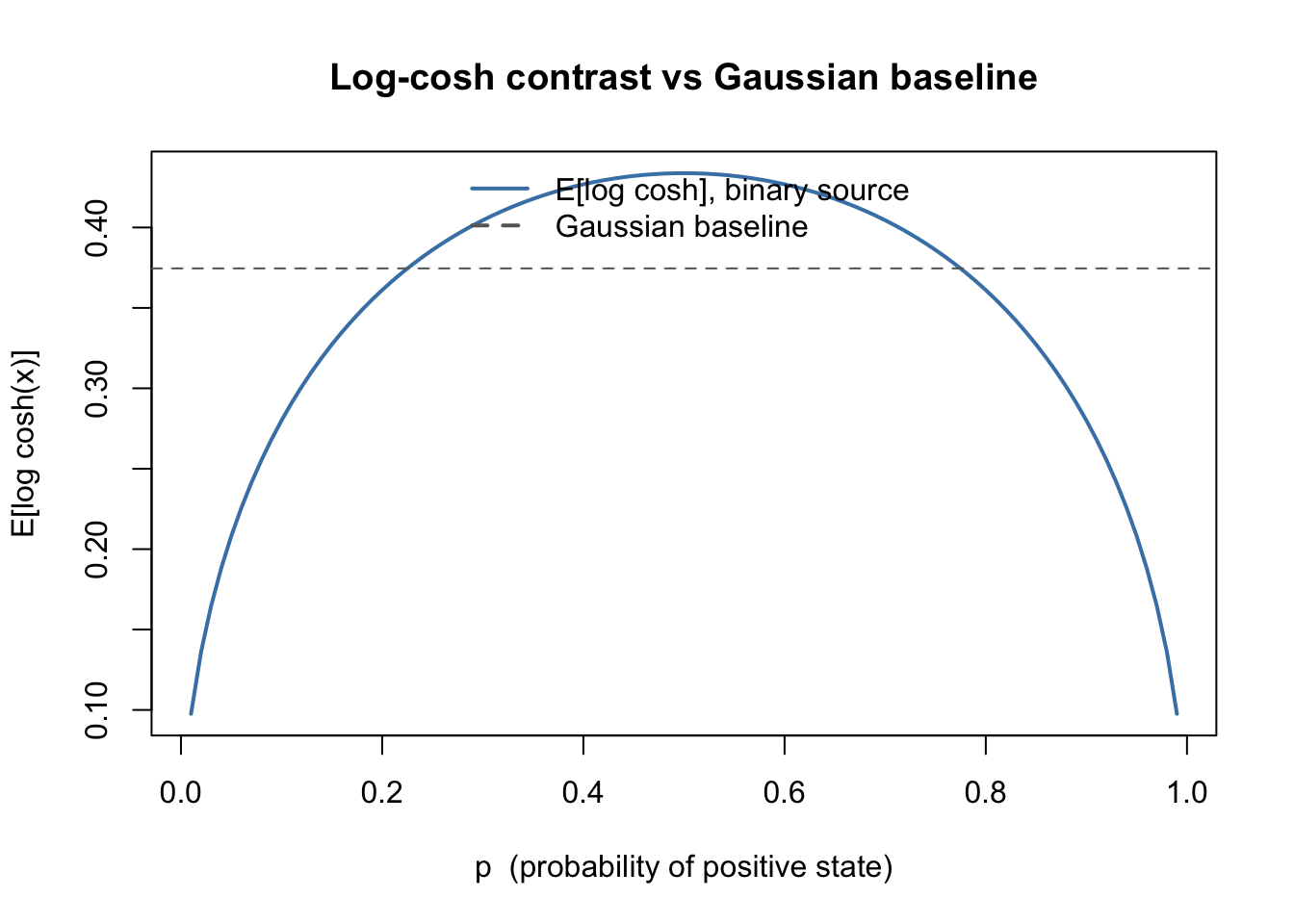
0.5\)), the expected log-cosh contrast falls
below the Gaussian baseline, causing fastICA to
actively avoid the true source direction.
This analysis generalizes the framework to an
asymmetric Rademacher prior parameterized by its
up-probability \(p\). We alternate
between:
Updating the projection direction \(w\) via a Newton-like fixed-point step (for
fixed \(p\)).
Updating \(p\) by maximizing the
marginal log-likelihood (for fixed \(w\)).
At \(p = 0.5\) the algorithm exactly
reduces to standard log-cosh fastICA. Two scale anchors are
compared:
M-estimator (\(c =
s\)): robust but slightly over-inflated variance.
Golden-ratio (\(c \approx
0.618\,s\)): satisfies \(c^2 + cs =
s^2\), so the assumed generative variance equals the empirical
data variance.
Helpers
prewhiten = function(X, n.comp) {
  X = X - rowMeans(X)
  sqrt(ncol(X)) * t(svd(X)$v[, 1:n.comp])
}
Implementation
With \(\sigma^2 = cs\), the score
function and its derivative are:
The Newton-like fixed-point update for \(w\) follows the standard fastICA pattern:
\[w \leftarrow \tfrac{1}{n}Y M(x) -
\overline{M'(x)}\,w, \qquad
w \leftarrow w / \|w\|\]
fastica_asym_r1 = function(Y, s = 1, anchor = c("M", "golden"),
                            tol = 1e-6, max_iter = 500, eps = 0.01,
                            w_init = NULL) {
  anchor = match.arg(anchor)
  c      = if (anchor == "M") s else s * (sqrt(5)-1)/2
  m = nrow(Y); n = ncol(Y)
  w = if (is.null(w_init)) rnorm(m) else w_init
  w = w / sqrt(sum(w^2))
  p = 0.5
  for (iter in seq_len(max_iter)) {
    w_old = w; p_old = p
    x  = as.vector(t(Y) %*% w)
    sc = asym_score(x, p, c, s)
    w  = as.vector(Y %*% sc$M) / n - mean(sc$Mp) * w
    w  = w / sqrt(sum(w^2))
    x   = as.vector(t(Y) %*% w)
    opt = optimize(\(pp) asym_obj_p(pp, x, c, s), c(eps, 1-eps), maximum = TRUE)
    p   = opt$maximum
    if (1 - abs(sum(w * w_old)) < tol && abs(p - p_old) < tol) break
  }
  list(w = w, p = p, iter = iter, c = c)
}
Standard log-cosh fastICA for comparison:
fastica_r1update = function(X, w) {
  w = w / sqrt(sum(w^2))
  P = t(X) %*% w
  G  = tanh(P); G2 = 1 - tanh(P)^2
  w  = X %*% G - mean(G2) * ncol(X) * w
  w / sqrt(sum(w^2))
}

run_seeds_lc = function(Y, S_true, n_seeds = 100, n_iter = 200) {
  maxcor = numeric(n_seeds)
  for (seed in seq_len(n_seeds)) {
    set.seed(seed)
    w = rnorm(nrow(Y))
    for (i in seq_len(n_iter)) w = fastica_r1update(Y, w)
    maxcor[seed] = max(abs(cor(t(S_true), t(Y) %*% w)))
  }
  maxcor
}

run_seeds_asym = function(Y, S_true, anchor, n_seeds = 100) {
  maxcor = numeric(n_seeds); ps = numeric(n_seeds)
  for (seed in seq_len(n_seeds)) {
    set.seed(seed)
    res = fastica_asym_r1(Y, anchor = anchor, w_init = rnorm(nrow(Y)))
    maxcor[seed] = max(abs(cor(t(S_true), t(Y) %*% res$w)))
    ps[seed]     = min(res$p, 1 - res$p)   # probability of the rare state
  }
  list(maxcor = maxcor, p = ps)
}

# Warm-start variant: run log-cosh to convergence, then hand off to asymmetric
run_seeds_asym_warm = function(Y, S_true, anchor, n_seeds = 100,
                                n_iter_lc = 200) {
  maxcor = numeric(n_seeds); ps = numeric(n_seeds)
  for (seed in seq_len(n_seeds)) {
    set.seed(seed)
    w = rnorm(nrow(Y))
    for (i in seq_len(n_iter_lc)) w = fastica_r1update(Y, w)
    res = fastica_asym_r1(Y, anchor = anchor, w_init = w)
    maxcor[seed] = max(abs(cor(t(S_true), t(Y) %*% res$w)))
    ps[seed]     = min(res$p, 1 - res$p)
  }
  list(maxcor = maxcor, p = ps)
}
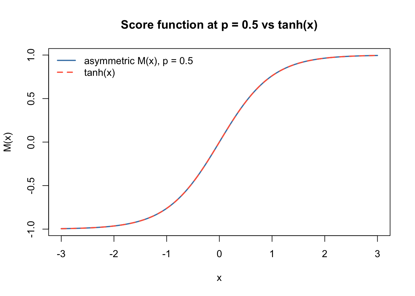
Sanity check: \(p = 0.5\) recovers
log-cosh
At \(p = 0.5\), \(s = 1\): \(\Delta(x) = 2x\), \(\pi(x) = (1 + \tanh x)/2\), and \(M(x) = \tanh(x)\) — the standard fastICA
score.
x_grid = seq(-3, 3, length.out = 300)
sc05   = asym_score(x_grid, p = 0.5, c = 1, s = 1)

plot(x_grid, sc05$M, type = "l", col = "steelblue", lwd = 2,
     xlab = "x", ylab = "M(x)",
     main = "Score function at p = 0.5 vs tanh(x)")
lines(x_grid, tanh(x_grid), col = "tomato", lty = 2, lwd = 2)
legend("topleft", c("asymmetric M(x), p = 0.5", "tanh(x)"),
       col = c("steelblue", "tomato"), lty = c(1, 2), lwd = 2, bty = "n")
Standard fastICA with log-cosh actively avoids
sources with $p < $ about \(0.1\) or
\(p > 0.9\): the contrast falls
below the Gaussian baseline, so the algorithm prefers noise directions
over the true source.
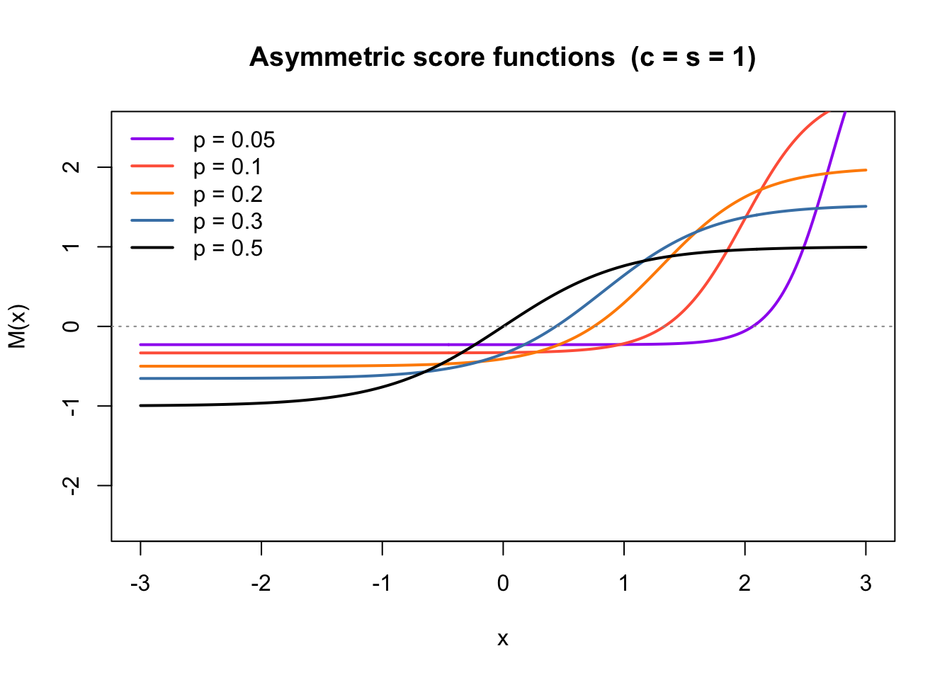
Score functions for varying \(p\)
As \(p\) decreases below 0.5 the
score shifts and steepens, penalising the positive tail more heavily —
appropriate for sources that are rarely “on”.
pvec2 = c(0.05, 0.1, 0.2, 0.3, 0.5)
cols  = c("purple", "tomato", "darkorange", "steelblue", "black")
plot(NULL, xlim = c(-3, 3), ylim = c(-2.5, 2.5),
     xlab = "x", ylab = "M(x)",
     main = "Asymmetric score functions  (c = s = 1)")
for (i in seq_along(pvec2))
  lines(x_grid, asym_score(x_grid, pvec2[i], 1, 1)$M, col = cols[i], lwd = 2)
legend("topleft", paste0("p = ", pvec2), col = cols, lwd = 2, bty = "n")
abline(h = 0, lty = 3, col = "grey60")
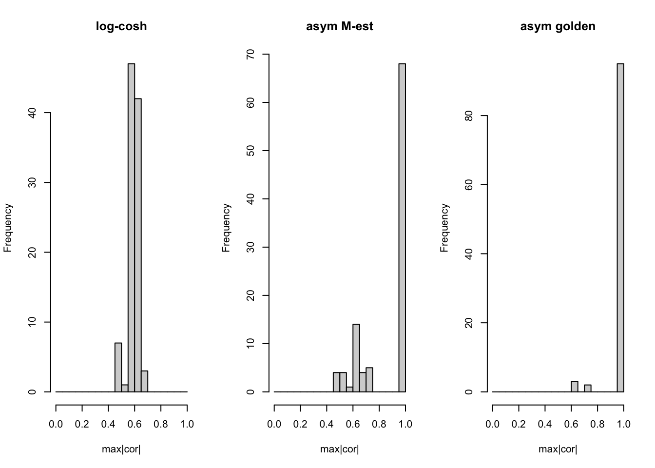
Log-cosh fails completely (all max|cor| < 0.9). The asymmetric
golden-ratio anchor nearly perfectly succeeds; the M-estimator anchor is
intermediate.
Why does the golden-ratio anchor do better?
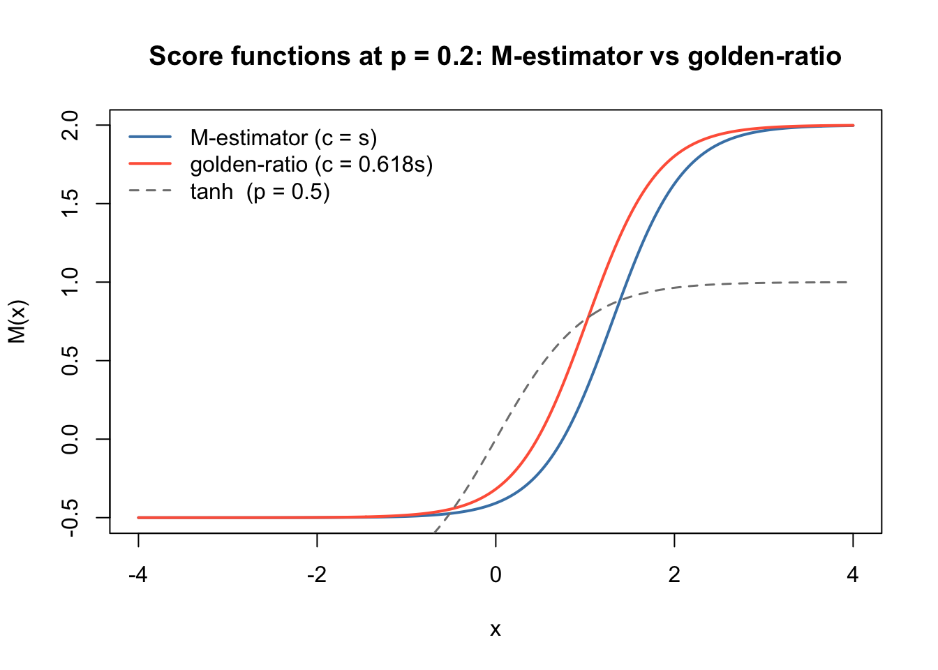
The two anchors produce different score functions via the \(c\)-dependent bias term in \(\Delta(x)\). The golden-ratio anchor (\(c = 0.618s\)) satisfies \(c^2 + cs = s^2\), so the total assumed
generative variance matches the empirical variance \(s^2\). The M-estimator (\(c = s\)) over-inflates the assumed variance
to \(2s^2\), shifting the logistic
midpoint and softening the asymmetry penalty.
We can visualise this: at \(p =
0.2\), \(s = 1\), the two
anchors produce noticeably different score functions:
x_grid2 = seq(-4, 4, length.out = 400)
sc_M  = asym_score(x_grid2, p = 0.2, c = 1,              s = 1)
sc_gr = asym_score(x_grid2, p = 0.2, c = (sqrt(5)-1)/2,  s = 1)

plot(x_grid2, sc_M$M,  type = "l", col = "steelblue", lwd = 2,
     xlab = "x", ylab = "M(x)",
     main = "Score functions at p = 0.2: M-estimator vs golden-ratio")
lines(x_grid2, sc_gr$M, col = "tomato", lwd = 2)
lines(x_grid2, tanh(x_grid2), col = "grey50", lty = 2, lwd = 1.5)
legend("topleft",
       c("M-estimator (c = s)", "golden-ratio (c = 0.618s)", "tanh  (p = 0.5)"),
       col = c("steelblue", "tomato", "grey50"),
       lty = c(1, 1, 2), lwd = c(2, 2, 1.5), bty = "n")
cat(sprintf("  asym golden (random)   mean = %.3f   frac > 0.9 = %.2f   mean_p = %.3f\n",
    mean(mc_s_gr$maxcor),  mean(mc_s_gr$maxcor  > 0.9), mean(mc_s_gr$p)))
asym golden (random) mean = 0.888 frac > 0.9 = 0.77 mean_p = 0.377
cat(sprintf("  asym golden (warm)     mean = %.3f   frac > 0.9 = %.2f   mean_p = %.3f\n",
    mean(mc_s_grw$maxcor), mean(mc_s_grw$maxcor > 0.9), mean(mc_s_grw$p)))
asym golden (warm) mean = 0.995 frac > 0.9 = 0.99 mean_p = 0.447
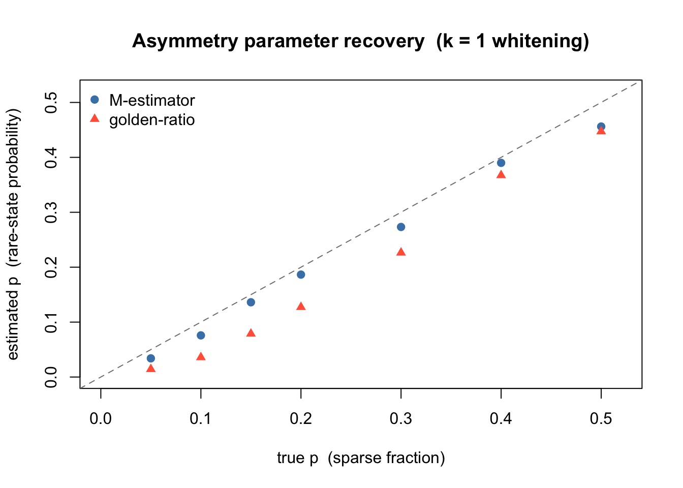
Asymmetry parameter recovery (\(k =
1\))
Using \(k = 1\) whitening (which
isolates each source exactly), we verify that the estimated \(\hat p\) tracks the true sparse fraction.
Because of sign ambiguity in the ICA direction, we report \(\min(\hat p,\, 1-\hat p)\), i.e. the
probability of the rare state.
Both anchors track the true sparse fraction closely across \(p \in [0.05, 0.5]\).
Summary
The asymmetric fastICA algorithm alternates between a Newton-like
fixed-point update for \(w\) (identical
to standard fastICA at \(p = 0.5\)) and
1D optimization of \(p\). Key findings
from 100 random seeds each:
Setting
log-cosh
asym golden (random)
asym golden (warm)
Symmetric Rademacher (\(p=0.5\),
\(k=9\))
0.99
0.77
0.99
9 overlapping groups (\(p \approx
0.2\), \(k=9\))
0.00
0.95
—
Log-cosh fails completely for the 9-groups case
because sparse sources have $E[] < $ Gaussian baseline, causing the
algorithm to prefer noise directions.
The golden-ratio anchor (\(c \approx 0.618s\)) dramatically
outperforms the M-estimator anchor. Its assumed generative variance
matches the empirical variance (\(c^2 + cs =
s^2\)), giving a better-calibrated asymmetry penalty.
The random-start degradation on symmetric sources is an
initialization artifact: the \(p\)-optimizer drifts from 0.5 before \(w\) has found a true source direction.
Warm-starting from a log-cosh solution (which already aligns \(w\) with a source) fully recovers the 99%
success rate, and the estimated \(\hat
p\) is close to 0.5.
Asymmetry recovery (\(k=1\) whitening): \(\hat p = \min(p, 1-p)\) correctly tracks
the true sparse fraction over the range \([0.05, 0.5]\).
Practical guidance: warm-starting from log-cosh is
a safe default — it matches log-cosh on symmetric sources and retains
the asymmetric method’s advantage when \(p\) is learned to be far from 0.5.