Examine susie and fsusie results on the ROSMAP data
William Denault, Hao Sun, Peter Carbonetto, Gao Wang
Last updated: 2024-06-20
Checks: 7 0
Knit directory:
fsusie-experiments/analysis/
This reproducible R Markdown analysis was created with workflowr (version 1.7.1.1). The Checks tab describes the reproducibility checks that were applied when the results were created. The Past versions tab lists the development history.
Great! Since the R Markdown file has been committed to the Git repository, you know the exact version of the code that produced these results.
Great job! The global environment was empty. Objects defined in the global environment can affect the analysis in your R Markdown file in unknown ways. For reproduciblity it’s best to always run the code in an empty environment.
The command set.seed(1) was run prior to running the
code in the R Markdown file. Setting a seed ensures that any results
that rely on randomness, e.g. subsampling or permutations, are
reproducible.
Great job! Recording the operating system, R version, and package versions is critical for reproducibility.
Nice! There were no cached chunks for this analysis, so you can be confident that you successfully produced the results during this run.
Great job! Using relative paths to the files within your workflowr project makes it easier to run your code on other machines.
Great! You are using Git for version control. Tracking code development and connecting the code version to the results is critical for reproducibility.
The results in this page were generated with repository version 73e153f. See the Past versions tab to see a history of the changes made to the R Markdown and HTML files.
Note that you need to be careful to ensure that all relevant files for
the analysis have been committed to Git prior to generating the results
(you can use wflow_publish or
wflow_git_commit). workflowr only checks the R Markdown
file, but you know if there are other scripts or data files that it
depends on. Below is the status of the Git repository when the results
were generated:
working directory clean
Note that any generated files, e.g. HTML, png, CSS, etc., are not included in this status report because it is ok for generated content to have uncommitted changes.
These are the previous versions of the repository in which changes were
made to the R Markdown (analysis/rosmap.Rmd) and HTML
(docs/rosmap.html) files. If you’ve configured a remote Git
repository (see ?wflow_git_remote), click on the hyperlinks
in the table below to view the files as they were in that past version.
| File | Version | Author | Date | Message |
|---|---|---|---|---|
| Rmd | 73e153f | Peter Carbonetto | 2024-06-20 | Added more descriptive text to the rosmap analysis. |
| Rmd | 2618c4e | Peter Carbonetto | 2024-06-20 | Adding some description of the results to the rosmap analysis. |
| html | b25a0af | Peter Carbonetto | 2024-06-18 | Build site. |
| Rmd | 0990217 | Peter Carbonetto | 2024-06-18 | Made a few minor improvements to the rosmap analysis (rosmap.Rmd). |
| Rmd | ace5ba7 | Peter Carbonetto | 2024-06-18 | Another small fix to the distance-to-TSS plot. |
| Rmd | aaf41ba | Peter Carbonetto | 2024-06-18 | Small fix to compute_weighted_distance_to_tss and a fix to the distance-to-TSS plot. |
| Rmd | 41c402c | Peter Carbonetto | 2024-06-18 | Small fix to the rosmap analysis. |
| Rmd | 0d322c4 | Peter Carbonetto | 2024-06-18 | Small edit to rosmap.Rmd. |
| Rmd | eed04e6 | Peter Carbonetto | 2024-05-03 | Small edit to rosmap.Rmd. |
| Rmd | 885d9a8 | Peter Carbonetto | 2024-05-03 | Added steps to rosmap.Rmd to assess overlap in ‘high-confidence’ causal SNPs. |
| Rmd | f7c26c8 | Peter Carbonetto | 2024-05-03 | A few tweaks to some of the histograms in rosmap.Rmd. |
| Rmd | b8e144c | Peter Carbonetto | 2024-05-03 | Updated the distance-to-tss plot in the rosmap analysis. |
| Rmd | 2520ca9 | Peter Carbonetto | 2024-05-03 | A few adjustments to some of the plots of the susie results in the rosmap analysis. |
| Rmd | 0ac5e4f | Peter Carbonetto | 2024-05-02 | Switched to a different set of susie results in the rosmap analysis. |
| Rmd | f4a0d35 | Peter Carbonetto | 2024-04-30 | Small change to one of the code chunks in rosmap.Rmd. |
| Rmd | 72b0109 | Peter Carbonetto | 2024-04-30 | Working on overlap calculations in rosmap analysis. |
| html | b5b3427 | Peter Carbonetto | 2024-04-29 | Rebuilt the rosmap analysis with the various updates mentioned in previous commits. |
| Rmd | 43aa3e2 | Peter Carbonetto | 2024-04-29 | workflowr::wflow_publish("rosmap.Rmd", view = FALSE, verbose = TRUE) |
| Rmd | 286a00d | Peter Carbonetto | 2024-04-29 | Implemented functions get_cs_sizes_by_region and cs_sizes_histogram for rosmap analysis. |
| Rmd | 9b6b1ee | Peter Carbonetto | 2024-04-29 | Merge branch ‘main’ of github.com:stephenslab/fsusie-experiments into main |
| Rmd | ed3a021 | Peter Carbonetto | 2024-04-29 | Implemented functions region_sizes_histogram and num_snps_histogram for rosmap analysis. |
| Rmd | 1f5e58e | Peter Carbonetto | 2024-04-29 | Working on identifying overlap in eqtl and mqtl susie/fsusie results. |
| Rmd | 357ccec | Peter Carbonetto | 2024-04-27 | Added histogram of CS sizes for fsusie mqtl results. |
| Rmd | 9f4070b | Peter Carbonetto | 2024-04-27 | Added a couple plots for fine-mapping of mqtl data to rosmap analysis. |
| Rmd | 259ebed | Peter Carbonetto | 2024-04-26 | Added a couple to-dos to the rosmap.Rmd. |
| html | ef4a009 | Peter Carbonetto | 2024-04-26 | Working on the rosmap analysis. |
| Rmd | b316ab6 | Peter Carbonetto | 2024-04-26 | workflowr::wflow_publish("rosmap.Rmd", verbose = TRUE, view = FALSE) |
| Rmd | cc246fe | Peter Carbonetto | 2024-04-26 | workflowr::wflow_publish("rosmap.Rmd", verbose = TRUE) |
| Rmd | 95e4aba | Peter Carbonetto | 2024-04-26 | Fixed the distance-to-TSS plot in the rosmap analysis. |
| Rmd | 366e27c | Peter Carbonetto | 2024-04-26 | Added a couple todos to rosmap.Rmd. |
| Rmd | e691fcd | Peter Carbonetto | 2024-04-26 | Added distance-to-TSS plot in the rosmap analysis. |
| Rmd | 4fb83bd | Peter Carbonetto | 2024-04-25 | Added step to rosmap.Rmd to get TSS for each ‘region’ in susie results. |
| Rmd | f8799a1 | Peter Carbonetto | 2024-04-25 | Added plot to rosmap.Rmd for CS sizes. |
| Rmd | 4ac6873 | Peter Carbonetto | 2024-04-25 | Added a couple simple plots to the rosmap analysis. |
| Rmd | 5ba241b | Peter Carbonetto | 2024-04-25 | Wrote function get_gene_annotations used in the rosmap analysis. |
| Rmd | b1b38f0 | Peter Carbonetto | 2024-04-25 | Added steps to rosmap analysis to prepare the gene annotations into a convenient data frame. |
| html | 142928b | Peter Carbonetto | 2024-04-25 | First build of rosmap analysis; added gene annotation files. |
| Rmd | a4e3d76 | Peter Carbonetto | 2024-04-25 | workflowr::wflow_publish("analysis/rosmap.Rmd", verbose = TRUE) |
Here we take a close look at a selection of the susie and fsusie fine-mapping results for the ROSMAP data.
Note: build the workflowr page, I ran these commands on midway2:
sinteractive -c 4 --mem=24G --time=20:00:00
module load R/4.1.0-no-openblas
module load pandoc/3.0.1
R
> .libPaths()[1]
# [1] "/home/pcarbo/R_libs_4_10_no_openblas"
> getwd()
# [1] "../analysis"
> workflowr::wflow_build("rosmap.Rmd",local=TRUE,view=FALSE,verbose=TRUE)
Load the packages as well as some additional custom functions used in the analysis below.
library(data.table)
library(ggplot2)
library(cowplot)
source("../code/rosmap_functions.R")
setDTthreads(1)
Load the susie fine-mapping results on the DLPFC bulk RNA-seq data.
datadir <- file.path("/project2/mstephens/fungen_xqtl/ftp_fgc_xqtl",
                     "analysis_result/finemapping_twas/prepared_results")
load(file.path(datadir,"susie_dlpfc_dejager_eQTL.RData"))
susie <- list(regions = regions,cs = cs,pips = pips)
susie$cs <- transform(susie$cs,pos = get_pos_from_id(id))
rm(regions,cs,pips)
Load the fsusie fine-mapping results on the DLPFC methylation data.
load(file.path(datadir,"fsusie_ROSMAP_DLPFC_mQTL.RData"))
fsusie_mqtl <- list(regions = regions,cs = cs,pips = pips)
rm(regions,cs,pips)
Load the fsusie fine-mapping results on the DLPFC histone acetylation (H3K9ac ChIP-seq) data.
load(file.path(datadir,"fsusie_ROSMAP_DLPFC_haQTL.RData"))
fsusie_haqtl <- list(regions = regions,cs = cs,pips = pips)
rm(regions,cs,pips)
Load the gene annotations. Specifically I extract here only the annotated gene transcripts for protein-coding genes as defined in the Ensembl/Havana database.
gene_file <-
  file.path("../data/genome_annotations",
    "Homo_sapiens.GRCh38.103.chr.reformatted.collapse_only.gene.gtf.gz")
genes <- get_gene_annotations(gene_file)
SuSiE fine-mapping of RNA-seq
Region sizes in base-pairs and SNPs:
p1 <- region_sizes_histogram(susie$regions,susie$pips,max_mb = 12)
p2 <- num_snps_histogram(susie$regions)
plot_grid(p1,p2)
# 54 regions are larger than 12 Mb.Most of the fine-mapping regions do not contain any CSs. Among the ones that have at least 1 CS, most contain 1 CS:
num_cs <- susie$regions$num_cs
table(CSs = num_cs)
num_cs <- num_cs[num_cs > 0]
pdat <- data.frame(num_cs = factor(num_cs))
ggplot(pdat,aes(num_cs)) +
  geom_bar(color = "white",fill = "darkblue",width = 0.5) +
  labs(x = "number of CSs",y = "number of regions") +
  theme_cowplot(font_size = 10)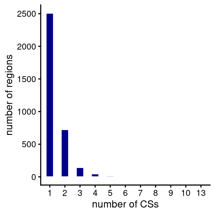
| Version | Author | Date |
|---|---|---|
| b25a0af | Peter Carbonetto | 2024-06-18 |
# CSs
#    0    1    2    3    4    5    6    7    8    9   10   13
# 4937 2508  725  144   47   18   10    9    3    1    1    1
A large number of the CSs predict a single causal SNP:
susie_cs_sizes <- get_cs_sizes_by_region(susie$cs)
cs_sizes_histogram(susie_cs_sizes,x_breaks = c(1:5,10,100,1000))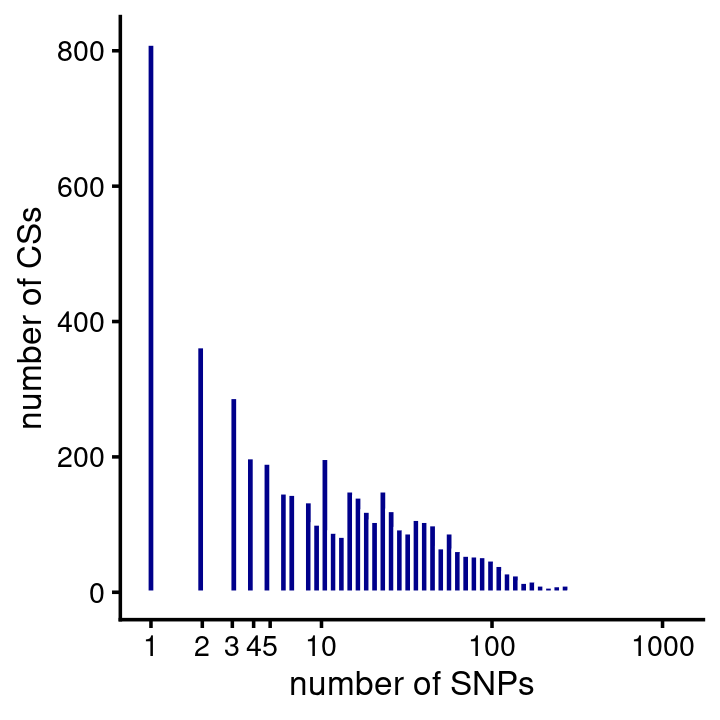
Plot showing distance between the susie SNP and the gene’s TSS, in which the distances are weighted by the PIPs (this is based only on SNPs that are in CSs). As expected, most of the predicted causal SNPs are very close to the nearest TSS.
susie$regions <- add_tss_to_regions(susie$regions,genes)
bin_size <- 25000
bins   <- c(-Inf,seq(-1e6,1e6,bin_size),Inf)
counts <- compute_weighted_distance_to_tss(susie$regions,susie$cs,bins)
n      <- length(bins)
bins   <- bins[seq(2,n-2)]
counts <- counts[seq(2,n-2)]
pdat <- data.frame(pos = (bins + bin_size/2)/1e6,count = counts)
ggplot(pdat,aes(x = pos,y = count)) +
  geom_point(color = "darkblue") +
  geom_line(color = "darkblue") +
  labs(x = "distance to TSS (Mb)",
       y = "SNPs weighted by PIP") +
  theme_cowplot(font_size = 10)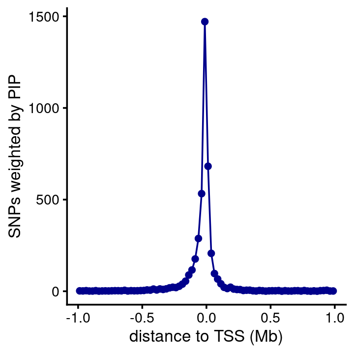
| Version | Author | Date |
|---|---|---|
| b25a0af | Peter Carbonetto | 2024-06-18 |
fSuSiE fine-mapping of haQTLs
The fSuSiE analyses typically involve much larger regions than the SuSiE analyses. The fSuSiE regions contain thousands of SNPs spanning several Mb:
p1 <- region_sizes_histogram(fsusie_haqtl$regions,fsusie_haqtl$pips,
                             max_mb = 10)
p2 <- num_snps_histogram(fsusie_haqtl$regions,max_snps = 50000)
plot_grid(p1,p2)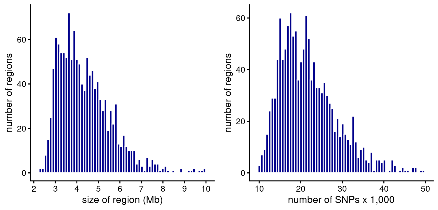
# 8 regions are larger than 10 Mb.
# 8 regions have more than 50000 SNPs.
fSuSiE usually identified at least one CS in a region, and most regions contain several CSs:
num_cs <- fsusie_haqtl$regions$num_cs
table(CSs = num_cs)
num_cs <- num_cs[num_cs > 0]
pdat <- data.frame(num_cs = factor(num_cs))
ggplot(pdat,aes(num_cs)) +
  geom_bar(color = "white",fill = "darkblue",width = 0.5) +
  labs(x = "number of CSs",y = "number of regions") +
  theme_cowplot(font_size = 10)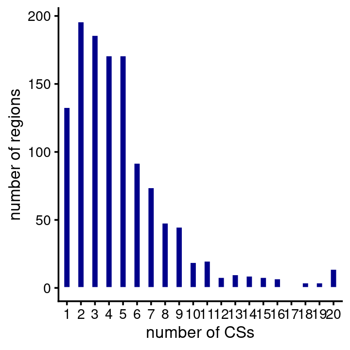
| Version | Author | Date |
|---|---|---|
| b25a0af | Peter Carbonetto | 2024-06-18 |
# CSs
#   0   1   2   3   4   5   6   7   8   9  10  11  12  13  14  15  16  17  18  19
#  85 133 196 186 171 171  92  74  48  45  19  20   8  10   9   8   7   1   4   4
#  20
#  14
The majority of the CSs predict a single causal SNP (note both the X and Y axes are on the log-scale):
fsusie_haqtl_cs_sizes <- get_cs_sizes_by_region(fsusie_haqtl$cs)
cs_sizes_histogram(fsusie_haqtl_cs_sizes,x_breaks = c(1:5,10,100,1000)) +
  scale_y_continuous(trans = "log10")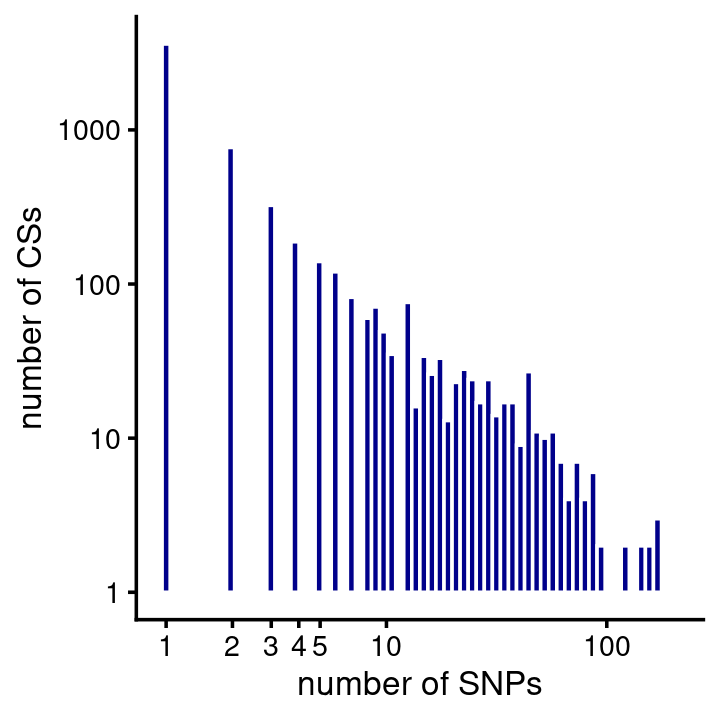
| Version | Author | Date |
|---|---|---|
| b5b3427 | Peter Carbonetto | 2024-04-29 |
fSuSiE fine-mapping of mQTLs
Now let’s examine the fSuSie methylation fine-mapping results. The regions are similar (but not exactly the same) to the fSuSiE analyses of HA:
p1 <- region_sizes_histogram(fsusie_mqtl$regions,fsusie_mqtl$pips,
                             max_mb = 10)
p2 <- num_snps_histogram(fsusie_mqtl$regions,max_snps = 50000)
plot_grid(p1,p2)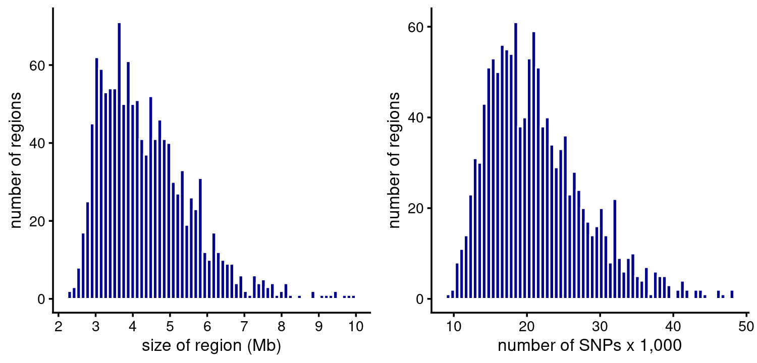
# 8 regions are larger than 10 Mb.
# 5 regions have more than 50000 SNPs.
In contrast to HA, a region typically contains many CSs, and all regions contain at least one CS. (Probably we could have identified more CSs if we had not limited the fSuSiE analyses to 20 CSs.)
num_cs <- fsusie_mqtl$regions$num_cs
table(CSs = num_cs)
num_cs <- num_cs[num_cs > 0]
pdat <- data.frame(num_cs = factor(num_cs))
ggplot(pdat,aes(num_cs)) +
  geom_bar(color = "white",fill = "darkblue",width = 0.5) +
  labs(x = "number of CSs",y = "number of regions") +
  theme_cowplot(font_size = 10)
| Version | Author | Date |
|---|---|---|
| b25a0af | Peter Carbonetto | 2024-06-18 |
# CSs
#   4   5   6   7   8   9  10  11  12  13  14  15  16  17  18  19  20
#   3   6   2   5  10  19  10  13  16  15  26  23  54  12  45 163 871
Similar to HA, most of the CSs contained just a single putative causal SNP (note again both the X and Y axes are on the log-scale):
fsusie_mqtl_cs_sizes <- get_cs_sizes_by_region(fsusie_mqtl$cs)
cs_sizes_histogram(fsusie_mqtl_cs_sizes,x_breaks = c(1:5,10,100,1000)) +
  scale_y_continuous(trans = "log10")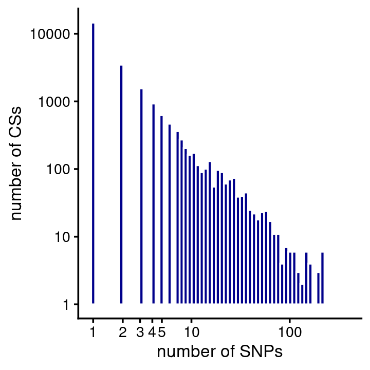
| Version | Author | Date |
|---|---|---|
| b5b3427 | Peter Carbonetto | 2024-04-29 |
Examine overlap among expression, methylation and histone acetylation SNPs
TO DO: Determine overlap between expression, methylation and histone acetylation SNPs simply by extracting the SNPs with PIP > 0.75 that are also in CSs.
highconf_susie <- get_highconf_snps(susie$pips,level = 0.6)
highconf_mqtl  <- get_highconf_snps(fsusie_mqtl$pips,level = 0.6)
highconf_haqtl <- get_highconf_snps(fsusie_haqtl$pips,level = 0.6)
ids <- unique(c(highconf_susie$id,highconf_mqtl$id,highconf_haqtl$id))
dat <- data.frame(id = ids,
                  eqtl  = is.element(ids,highconf_susie$id),
                  mqtl  = is.element(ids,highconf_mqtl$id),
                  haqtl = is.element(ids,highconf_haqtl$id))
table(dat[c("eqtl","mqtl")])
table(dat[c("eqtl","haqtl")])
table(dat[c("mqtl","haqtl")])
TO DO NEXT: Put together a data frame containing more information about these high-confidence, overlapping SNPs.
sessionInfo()
# R version 4.1.0 (2021-05-18)
# Platform: x86_64-pc-linux-gnu (64-bit)
# Running under: CentOS Linux 7 (Core)
#
# Matrix products: default
# BLAS:   /software/R-4.1.0-no-openblas-el7-x86_64/lib64/R/lib/libRblas.so
# LAPACK: /software/R-4.1.0-no-openblas-el7-x86_64/lib64/R/lib/libRlapack.so
#
# locale:
#  [1] LC_CTYPE=en_US.UTF-8       LC_NUMERIC=C
#  [3] LC_TIME=en_US.UTF-8        LC_COLLATE=en_US.UTF-8
#  [5] LC_MONETARY=en_US.UTF-8    LC_MESSAGES=en_US.UTF-8
#  [7] LC_PAPER=en_US.UTF-8       LC_NAME=C
#  [9] LC_ADDRESS=C               LC_TELEPHONE=C
# [11] LC_MEASUREMENT=en_US.UTF-8 LC_IDENTIFICATION=C
#
# attached base packages:
# [1] stats     graphics  grDevices utils     datasets  methods   base
#
# other attached packages:
# [1] cowplot_1.1.1     ggplot2_3.5.1     data.table_1.14.0
#
# loaded via a namespace (and not attached):
#  [1] tidyselect_1.1.1  xfun_0.24         bslib_0.4.2       purrr_0.3.4
#  [5] colorspace_2.0-2  vctrs_0.6.5       generics_0.1.0    htmltools_0.5.5
#  [9] yaml_2.2.1        utf8_1.2.1        rlang_1.1.1       R.oo_1.24.0
# [13] jquerylib_0.1.4   later_1.2.0       pillar_1.6.1      glue_1.4.2
# [17] withr_2.5.0       DBI_1.1.1         R.utils_2.10.1    lifecycle_1.0.3
# [21] stringr_1.4.0     munsell_0.5.0     gtable_0.3.0      workflowr_1.7.1.1
# [25] R.methodsS3_1.8.1 evaluate_0.14     labeling_0.4.2    knitr_1.33
# [29] fastmap_1.1.0     httpuv_1.6.1      fansi_0.5.0       highr_0.9
# [33] Rcpp_1.0.12       promises_1.2.0.1  scales_1.3.0      cachem_1.0.5
# [37] jsonlite_1.7.2    farver_2.1.0      fs_1.5.0          digest_0.6.27
# [41] stringi_1.6.2     dplyr_1.0.7       rprojroot_2.0.2   grid_4.1.0
# [45] cli_3.6.1         tools_4.1.0       magrittr_2.0.1    sass_0.4.0
# [49] tibble_3.1.2      crayon_1.4.1      whisker_0.4       pkgconfig_2.0.3
# [53] ellipsis_0.3.2    assertthat_0.2.1  rmarkdown_2.9     R6_2.5.0
# [57] git2r_0.28.0      compiler_4.1.0