Examine methylation and H3K27ac fine-mapping results from the ROSMAP data
William Denault, Hao Sun, Angjing Liu, Peter Carbonetto, Gao Wang
Last updated: 2025-03-27
Checks: 6 1
Knit directory:
fsusie-experiments/analysis/
This reproducible R Markdown analysis was created with workflowr (version 1.7.1). The Checks tab describes the reproducibility checks that were applied when the results were created. The Past versions tab lists the development history.
Great! Since the R Markdown file has been committed to the Git repository, you know the exact version of the code that produced these results.
Great job! The global environment was empty. Objects defined in the global environment can affect the analysis in your R Markdown file in unknown ways. For reproduciblity it’s best to always run the code in an empty environment.
The command set.seed(1) was run prior to running the
code in the R Markdown file. Setting a seed ensures that any results
that rely on randomness, e.g. subsampling or permutations, are
reproducible.
Great job! Recording the operating system, R version, and package versions is critical for reproducibility.
- get-cpgs-per-tad-assoc
To ensure reproducibility of the results, delete the cache directory
rosmap_overview_cache and re-run the analysis. To have
workflowr automatically delete the cache directory prior to building the
file, set delete_cache = TRUE when running
wflow_build() or wflow_publish().
Great job! Using relative paths to the files within your workflowr project makes it easier to run your code on other machines.
Great! You are using Git for version control. Tracking code development and connecting the code version to the results is critical for reproducibility.
The results in this page were generated with repository version 2bd0de3. See the Past versions tab to see a history of the changes made to the R Markdown and HTML files.
Note that you need to be careful to ensure that all relevant files for
the analysis have been committed to Git prior to generating the results
(you can use wflow_publish or
wflow_git_commit). workflowr only checks the R Markdown
file, but you know if there are other scripts or data files that it
depends on. Below is the status of the Git repository when the results
were generated:
Untracked files:
    Untracked:  analysis/rosmap_overview_cache/
    Untracked:  data/analysis_result/Fungen_xQTL.ENSG00000163808.cis_results_db.export.rds
    Untracked:  data/analysis_result/ROSMAP_haQTL.chr3_43915257_48413435.fsusie_mixture_normal_top_pc_weights.rds
    Untracked:  data/analysis_result/ROSMAP_mQTL.chr3_43915257_48413435.fsusie_mixture_normal_top_pc_weights.rds
    Untracked:  outputs/ROSMAP_haQTL_cs_effect_ha_peak_annotation.tsv.gz
    Untracked:  outputs/ROSMAP_haQTL_cs_snp_annotation.tsv.gz
    Untracked:  outputs/ROSMAP_haQTL_cs_snp_toppc1_annotation.tsv.gz
    Untracked:  outputs/ROSMAP_haQTL_qtl_snp_qval0.05.tsv.gz
    Untracked:  outputs/ROSMAP_haQTL_qtl_snp_qval0.05_annotation.tsv.gz
    Untracked:  outputs/ROSMAP_mQTL_cs_effect_cpg_annotation.tsv.gz
    Untracked:  outputs/ROSMAP_mQTL_cs_snp_annotation.tsv.gz
    Untracked:  outputs/ROSMAP_mQTL_cs_snp_toppc1_annotation.tsv.gz
    Untracked:  outputs/ROSMAP_mQTL_qtl_snp_qval0.05.tsv.gz
    Untracked:  outputs/ROSMAP_mQTL_qtl_snp_qval0.05_annotation.tsv.gz
Note that any generated files, e.g. HTML, png, CSS, etc., are not included in this status report because it is ok for generated content to have uncommitted changes.
These are the previous versions of the repository in which changes were
made to the R Markdown (analysis/rosmap_overview.Rmd) and
HTML (docs/rosmap_overview.html) files. If you’ve
configured a remote Git repository (see ?wflow_git_remote),
click on the hyperlinks in the table below to view the files as they
were in that past version.
| File | Version | Author | Date | Message |
|---|---|---|---|---|
| Rmd | 2bd0de3 | Peter Carbonetto | 2025-03-27 | wflow_publish("rosmap_overview.Rmd", verbose = TRUE, view = FALSE) |
| Rmd | 53d4a33 | Peter Carbonetto | 2025-03-27 | Added code chunks to rosmap_overview.Rmd for generating PDFs of some of the plots. |
| Rmd | d5c9e37 | Peter Carbonetto | 2025-03-27 | A few fixes to rosmap_overview.Rmd. |
| Rmd | 544235d | Peter Carbonetto | 2025-03-27 | Added code chunks to save some of the plots in the rosmap_overview analysis. |
| html | aece910 | Peter Carbonetto | 2025-03-24 | Ran workflowr::wflow_publish("rosmap_overview.Rmd"). |
| Rmd | 0eb8295 | Peter Carbonetto | 2025-03-24 | wflow_publish("rosmap_overview.Rmd", view = FALSE, verbose = TRUE) |
| Rmd | 6de898e | Peter Carbonetto | 2025-03-24 | Added plots to the rosmap_overview analysis summarizing the recovery of affected H3K27ac peaks. |
| Rmd | 7c8d51d | Peter Carbonetto | 2025-03-24 | Added TSS plot for H3K27ac in rosmap_overview analysis. |
| Rmd | 8e17486 | Peter Carbonetto | 2025-03-24 | Added code to create a plot showing the density of causal SNPs near the closest TSS. |
| Rmd | 18c11b5 | Peter Carbonetto | 2025-03-24 | Added code to rosmap_overview.Rmd to load gene annotations. |
| Rmd | 60bbe23 | Peter Carbonetto | 2025-03-22 | Added a couple notes to the rosmap_summary analysis. |
| Rmd | 00bb89c | Peter Carbonetto | 2025-03-21 | Added note to rosmap_overview.Rmd. |
| Rmd | 7adfd4d | Peter Carbonetto | 2025-03-21 | A few fixes to the rosmap_overview analysis. |
| Rmd | c087a58 | Peter Carbonetto | 2025-03-21 | Added some notes to the rosmap_overview analysis. |
| Rmd | 5e9432b | Peter Carbonetto | 2025-03-21 | Added plots to the rosmap_overview analysis summarizing the affected CpGs identified by fSuSiE and the association tests. |
| Rmd | 593c7e0 | Peter Carbonetto | 2025-03-21 | Added some code for analyzing the HA peak results in the rosmap_overview analysis. |
| Rmd | 12ed0b1 | Peter Carbonetto | 2025-03-21 | Small fix. |
| Rmd | e663ab0 | Peter Carbonetto | 2025-03-21 | Added code to read in HA_peak results in rosmap_overview analysis. |
| html | 71954f1 | Peter Carbonetto | 2025-03-20 | Added plots summarizing H3K27ac results to rosmap_overview analysis. |
| Rmd | 1ad355a | Peter Carbonetto | 2025-03-20 | wflow_publish("rosmap_overview.Rmd", view = FALSE, verbose = TRUE) |
| html | c84e5c0 | Peter Carbonetto | 2025-03-20 | Rebuilt the rosmap_overview analysis with the new results. |
| Rmd | 1c8eeb7 | Peter Carbonetto | 2025-03-20 | wflow_publish("rosmap_overview.Rmd", view = FALSE) |
| Rmd | acfadd1 | Peter Carbonetto | 2025-03-20 | Made a few improvements to the code and text of the rosmap_analysis. |
| Rmd | c102af9 | Peter Carbonetto | 2025-03-20 | Added a scatterplot comparing number of CSs per TAD (susie vs. fsusie). |
| Rmd | 12f2fd3 | Peter Carbonetto | 2025-03-20 | Added some histograms on TAD CS sizes. |
| Rmd | c69e187 | Peter Carbonetto | 2025-03-20 | Created plot showing TAD sizes from the methylation fine-mapping results. |
| Rmd | 2a5c706 | Peter Carbonetto | 2025-03-20 | Added code to the rosmap_overview analysis to load the methylation SNP results. |
| Rmd | c3a01c7 | Peter Carbonetto | 2025-03-20 | Added link for downloading data to rosmap_overview analysis. |
| html | 5c446c0 | Peter Carbonetto | 2025-03-20 | First build of the rosmap_overview analysis. |
| Rmd | 7532908 | Peter Carbonetto | 2025-03-20 | workflowr::wflow_publish("rosmap_overview.Rmd", verbose = TRUE) |
| Rmd | bc6d0a1 | Peter Carbonetto | 2025-03-20 | Started working on rosmap_overview analysis. |
Note: If you would like to run this analysis on your computer, you will first need to download the fine-mapping outputs. They can be downloaded from here. Once you have downloaded the files, copy them to the “outputs” subdirectory.
Load some packges used in the code below:
library(data.table)
library(ggplot2)
library(cowplot)
This is a function I use to Extract the gene annotations from the GTF (“gene transfer format”) file. Here we keep only the annotated gene transcripts for protein-coding genes as defined in the Ensembl/Havana database.
get_gene_annotations <- function (gene_file) {
  out <- fread(file = gene_file,sep = "\t",header = FALSE,skip = 1)
  class(out) <- "data.frame"
  names(out) <- c("chromosome","source","feature","start","end","score",
                    "strand","frame","attributes")
  out <- out[c("chromosome","source","feature","start","end","strand",
               "attributes")]
  out <- transform(out,
                   chromosome = factor(chromosome),
                   source     = factor(source),
                   feature    = factor(feature),
                   strand     = factor(strand))
  out <- subset(out,
                source == "ensembl_havana" &
                feature == "transcript")
  out <-
    transform(out,
      ensembl   = sapply(strsplit(attributes,";"),
                         function (x) substr(x[[1]],10,24)),
      gene_type = sapply(strsplit(attributes,";"),
                         function (x) substr(x[[3]],13,nchar(x[[3]]) - 1)),
      gene_name = sapply(strsplit(attributes,";"),
                         function (x) substr(x[[4]],13,nchar(x[[4]]) - 1)))
  out <- out[-7]
  out <- transform(out,gene_type = factor(gene_type))
  out <- subset(out,gene_type == "protein_coding")
  rownames(out) <- NULL
  return(out)
}
Load the gene annotations which will be used in some of the analyses below. Specifically, I extract here only the annotated gene transcripts for protein-coding genes as defined in the Ensembl/Havana database.
gene_file <-
  file.path("../data/genome_annotations",
    "Homo_sapiens.GRCh38.103.chr.reformatted.collapse_only.gene.gtf.gz")
genes <- get_gene_annotations(gene_file)
Methylation SNPs
First, I define a helper function for loading the enrichment results:
# The "n" argument specifies the number of "meta data" columns.
# Columns after that are treated as the enrichment results. These
# columns contain only binary data (0 or 1) indicating whether or not
# the genomic feature (genetic variant or molecular trait location)
# is assigned that specific annotation.
read_enrichment_results <- function (filename, n) {
  out <- fread(filename,sep = "\t",stringsAsFactors = FALSE,header = TRUE)
  class(out) <- "data.frame"
  out <- transform(out,chr = factor(chr))
  if (ncol(out) > n) {
    cols <- seq(n + 1,ncol(out))
    for (i in cols)
      out[[i]] <- factor(out[[i]])
  }
  return(out)
}
Next I load methylation SNP results generated by SuSiE-topPC, fSuSiE and the SNP-CpG association testing:
methyl_cpg_assoc_file  <- "../outputs/ROSMAP_mQTL_qtl_snp_qval0.05.tsv.gz"
methyl_snps_susie_file <-
  "../outputs/ROSMAP_mQTL_cs_snp_toppc1_annotation.tsv.gz"
methyl_snps_fsusie_file <- "../outputs/ROSMAP_mQTL_cs_snp_annotation.tsv.gz"
methyl_snps_susie  <- read_enrichment_results(methyl_snps_susie_file,n = 6)
methyl_snps_fsusie <- read_enrichment_results(methyl_snps_fsusie_file,n = 7)
methyl_cpg_assoc   <- read_enrichment_results(methyl_cpg_assoc_file,n = 8)
methyl_snps_susie$region <-
  sapply(strsplit(methyl_snps_susie$cs,":",fixed = TRUE),"[[",2)
methyl_snps_susie  <- transform(methyl_snps_susie,
                                region = factor(region),
                                cs     = factor(cs),
                                pc     = factor(pc))
methyl_snps_fsusie <- transform(methyl_snps_fsusie,
                                cs     = factor(cs),
                                region = factor(region),
                                study  = factor(study))
This is the number of fine-mapping regions (TADs) that contained at least one CS in each of the analyses:
nlevels(methyl_snps_susie$region)
nlevels(methyl_snps_fsusie$region)
# [1] 1236
# [1] 1327
This is a function we will use below to get the sizes of the TADs (in Mb):
get_tad_sizes <- function (tads) {
  tads <- strsplit(tads,"_",fixed = TRUE)
  pos0 <- as.numeric(sapply(tads,"[[",2))
  pos1 <- as.numeric(sapply(tads,"[[",3))
  return((pos1 - pos0)/1e6)
}
This plot summarizes the sizes of the TADs that were analyzed by SuSiE-topPC and fSuSiE:
plot_tad_sizes <- function (tads) {
  tad_size <- get_tad_sizes(tads)
  pdat <- data.frame(tad_size = tad_size)
  return(ggplot(pdat,aes(x = tad_size)) +
         geom_histogram(color = "white",fill = "black",bins = 48) +
         labs(x = "size (Mb)",y = "number of TADs") +
         theme_cowplot(font_size = 10))
}
tads <- levels(methyl_snps_fsusie$region)
p <- plot_tad_sizes(tads) +
  scale_x_continuous(limits = c(2,9),breaks = 1:10) +
  scale_y_continuous(breaks = seq(0,100,10))
print(p)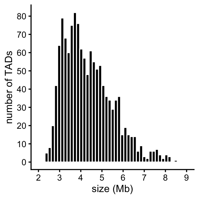
Some other useful statistics on the TAD sizes:
tad_size <- get_tad_sizes(tads)
length(tad_size)
range(tad_size)
mean(tad_size)
median(tad_size)
sum(tad_size > 9)
# [1] 1327
# [1]  2.320952 34.727189
# [1] 4.54465
# [1] 4.154266
# [1] 19
These histograms summarize the number of CSs per TAD:
get_cs_vs_tad_size <- function (dat) {
  tads <- levels(dat$region)
  out <- data.frame(tad      = tads,
                    tad_size = get_tad_sizes(tads),
                    num_cs   = tapply(dat$cs,dat$region,
                                      function (x) length(unique(x))))
  rownames(out) <- NULL
  return(out)
}
pdat1 <- get_cs_vs_tad_size(methyl_snps_susie)
pdat2 <- get_cs_vs_tad_size(methyl_snps_fsusie)
pdat1 <- transform(pdat1,num_cs = factor(num_cs,1:20))
pdat2 <- transform(pdat2,num_cs = factor(num_cs,1:20))
p1 <- ggplot(pdat1,aes(x = num_cs)) +
  geom_histogram(stat = "count",color = "white",fill = "darkblue") +
  scale_x_discrete(drop = FALSE) +
  labs(x = "number of CSs",y = "number of TADs",title = "SuSiE-topPC") +
  theme_cowplot(font_size = 10) +
  theme(plot.title = element_text(size = 10,face = "plain"))
p2 <- ggplot(pdat2,aes(x = num_cs)) +
  geom_histogram(stat = "count",color = "white",fill = "darkblue") +
  scale_x_discrete(drop = FALSE) +
  labs(x = "number of CSs",y = "number of TADs",title = "fSuSiE") +
  theme_cowplot(font_size = 10) +
  theme(plot.title = element_text(size = 10,face = "plain"))
plot_grid(p1,p2,nrow = 1,ncol = 2)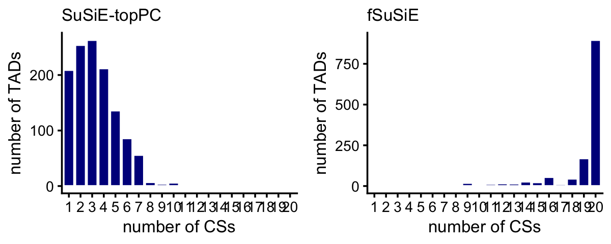
Compare discovery of causal SNPs (number of CSs) in the SuSiE-topPC and fSuSiE analyses:
dat1 <- get_cs_vs_tad_size(methyl_snps_susie)
dat2 <- get_cs_vs_tad_size(methyl_snps_fsusie)
dat1 <- dat1[c(1,3)]
dat2 <- dat2[c(1,3)]
names(dat1) <- c("tad","num_cs_susie")
names(dat2) <- c("tad","num_cs_fsusie")
dat <- merge(dat1,dat2,all = TRUE)
rows <- which(is.na(dat$num_cs_susie))
dat[rows,"num_cs_susie"] <- 0
pdat <- melt(with(dat,table(num_cs_susie,num_cs_fsusie)))
rows <- which(pdat$value == 0)
pdat[rows,"value"] <- NA
p <- ggplot(pdat,aes(x = num_cs_susie,y = num_cs_fsusie,size = value)) +
  geom_point(color = "white",fill = "darkblue",shape = 21) +
  geom_abline(intercept = 0,slope = 1,color = "black",linetype = "dotted") +
  scale_x_continuous(breaks = seq(0,20,2),limits = c(0,20)) +
  scale_y_continuous(breaks = seq(0,20,2),limits = c(0,20)) +
  scale_size(breaks = c(1,10,100)) +
  labs(x = "SuSiE-topPC",y = "fSuSiE",size = "number of TADs") +
  theme_cowplot(font_size = 10)
print(p)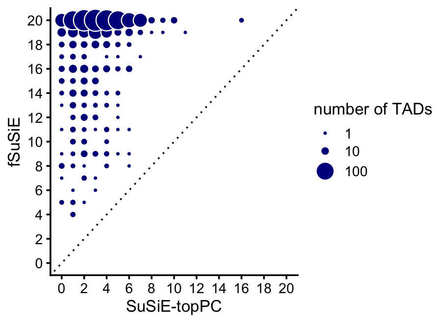
| Version | Author | Date |
|---|---|---|
| c84e5c0 | Peter Carbonetto | 2025-03-20 |
Compare the sizes of the CSs in the SuSiE-topPC and fSuSiE analyses:
bins <- c(0,1,2,5,10,20,Inf)
cs_size_susie  <- as.numeric(table(methyl_snps_susie$cs))
cs_size_fsusie <- as.numeric(table(methyl_snps_fsusie$cs))
cs_size_susie  <- cut(cs_size_susie,bins)
cs_size_fsusie <- cut(cs_size_fsusie,bins)
levels(cs_size_susie) <- bins[-1]
levels(cs_size_fsusie) <- bins[-1]
p1 <- ggplot(data.frame(cs_size = cs_size_susie),aes(x = cs_size)) +
  geom_histogram(stat = "count",color = "white",fill = "darkblue",
                 width = 0.65) +
  labs(x = "CS size",y = "number of CSs",title = "SuSiE-topPC") +
  theme_cowplot(font_size = 10) +
  theme(plot.title = element_text(size = 10,face = "plain"))
p2 <- ggplot(data.frame(cs_size = cs_size_fsusie),aes(x = cs_size)) +
  geom_histogram(stat = "count",color = "white",fill = "darkblue",
                 width = 0.65) +
  labs(x = "CS size",y = "number of CSs",title = "fSuSiE") +
  theme_cowplot(font_size = 10) +
  theme(plot.title = element_text(size = 10,face = "plain"))
plot_grid(p1,p2,nrow = 1,ncol = 2)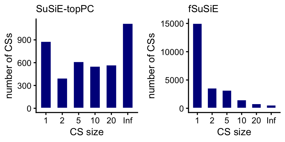
| Version | Author | Date |
|---|---|---|
| c84e5c0 | Peter Carbonetto | 2025-03-20 |
We expect that most of the causal SNPs to be very close to the nearest TSS. Let’s check this. This will involve a couple of intermediate calculations.
This function adds a column to the SNP results containing the minimum distance to the nearest TSS.
add_min_dist_to_tss <- function (dat, genes) {
  n <- nrow(dat)
  dat$min_dist_to_tss <- rep(Inf,n)
  n <- nrow(genes)
  for (i in 1:n) {
    rows <- which(as.character(genes[i,"chromosome"]) == as.character(dat$chr))
    if (length(rows) > 0) {
      if (genes[i,"strand"] == "+")
        d <- genes[i,"start"] - dat[rows,"pos"]
      else
        d <- dat[rows,"pos"] - genes[i,"end"]
      i <- which(abs(d) < abs(dat[rows,"min_dist_to_tss"]))
      if (length(i) > 0) {
        d    <- d[i]
        rows <- rows[i]
        dat[rows,"min_dist_to_tss"] <- d
      }
    }
  }
  return(dat)
}
This function is used to extract the top SNP per location (e.g., CpG) from the association tests.
get_top_snp_per_location <- function (dat) {
  x <- factor(dat$molecular_trait_id)
  qval <- dat$qvalue
  names(qval) <- with(dat,paste(chr,pos,sep = "_"))
  res <- tapply(qval,x,function (x) names(which.min(x)))
  res <- strsplit(res,"_",fixed = TRUE)
  out <- data.frame(chr = factor(sapply(res,"[[",1)),
                    pos = as.numeric(sapply(res,"[[",2)))
  out <- transform(out,chr = factor(chr))
  rownames(out) <- levels(x)
  return(out)
}
With these functions, we can compile the data needed for this plot.
methyl_snps_assoc  <- get_top_snp_per_location(methyl_cpg_assoc)
methyl_snps_assoc  <- add_min_dist_to_tss(methyl_snps_assoc,genes)
methyl_snps_susie  <- add_min_dist_to_tss(methyl_snps_susie,genes)
methyl_snps_fsusie <- add_min_dist_to_tss(methyl_snps_fsusie,genes)
For SuSiE-topPC and fSuSiE, we calculate “weighted” counts of SNPs, in which the weights are given by the PIPs.
bin_size <- 10000
bins <- c(-Inf,seq(-2e5,2e5,bin_size),Inf)
bins <- bins + bin_size/2
counts_assoc <- as.numeric(table(cut(methyl_snps_assoc$min_dist_to_tss,bins)))
counts_susie <- tapply(methyl_snps_susie$pip,
                       cut(methyl_snps_susie$min_dist_to_tss,bins),
                       function (x) sum(x,na.rm = TRUE))
counts_fsusie <- tapply(methyl_snps_fsusie$pip,
                        cut(methyl_snps_fsusie$min_dist_to_tss,bins),
                        function (x) sum(x,na.rm = TRUE))
Now we can plot the result:
n <- length(bins)
i <- seq(2,n-2)
bin_centers   <- bins[i] + bin_size/2
counts_assoc  <- counts_assoc[i]
counts_susie  <- counts_susie[i]
counts_fsusie <- counts_fsusie[i]
counts_assoc  <- counts_assoc/sum(counts_assoc)
counts_susie  <- counts_susie/sum(counts_susie)
counts_fsusie <- counts_fsusie/sum(counts_fsusie)
pdat <- data.frame(method = rep(c("assoc","susie","fsusie"),
                                each = length(bin_centers)),
                   dist   = rep(bin_centers/1000,times = 3),
                   freq   = c(counts_assoc,counts_susie,counts_fsusie),
                   stringsAsFactors = TRUE)
p <- ggplot(pdat,aes(x = dist,y = freq,color = method)) +
  geom_line(linewidth = 0.5) +
  geom_point(size = 1) +
  scale_x_continuous(breaks = seq(-200,200,50)) +
  scale_y_continuous(breaks = seq(0,1,0.05)) +
  scale_color_manual(values = c("darkblue","darkorange","dodgerblue")) +
  labs(x = "distance to TSS (kb)",y = "proportion of SNPs") +
  theme_cowplot(font_size = 10)
print(p)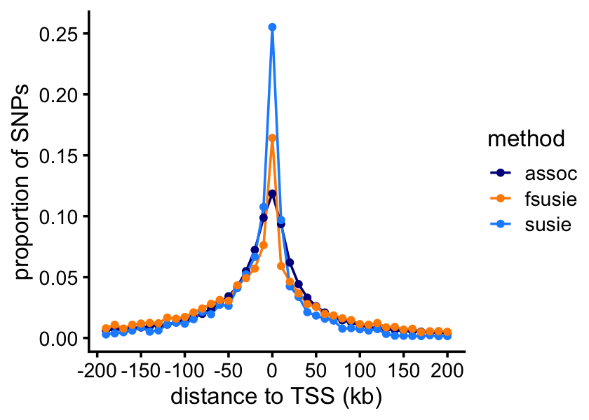
| Version | Author | Date |
|---|---|---|
| aece910 | Peter Carbonetto | 2025-03-24 |
Affected CpGs
Now let’s turn to the recovery of affected CpGs. Load the results generated by fSuSiE (the SNP-CpG association testing results were imported previously):
methyl_cpg_fsusie_file <-
  "../outputs/ROSMAP_mQTL_cs_effect_cpg_annotation.tsv.gz"
methyl_cpg_fsusie <- read_enrichment_results(methyl_cpg_fsusie_file,n = 9)
methyl_cpg_fsusie$region <-
  sapply(strsplit(methyl_cpg_fsusie$cs,":",fixed = TRUE),"[[",2)
methyl_cpg_fsusie <- transform(methyl_cpg_fsusie,
                               cs      = factor(cs),
                               region  = factor(region),
                               context = factor(context))
Counting the number of CpGs per TAD is quite simple from the way the fSuSiE results were compiled. It involves counting the number of unique CpGs in each TAD:
cpgs_per_tad_fsusie <-
  with(methyl_cpg_fsusie,tapply(ID,region,function (x) length(unique(x))))
Counting the number of CpGs per TAD from the SNP-CpG association tests is a little more complicated because the CpGs were not assigned to TADs in the results.
# Extract the information about the TADs from the TAD labels.
get_tad_info <- function (tads) {
  res <- strsplit(tads,"_")
  return(data.frame(tad   = tads,
                    chr   = factor(sapply(res,"[[",1)),
                    start = as.numeric(sapply(res,"[[",2)),
                    end   = as.numeric(sapply(res,"[[",3))))
}

# Count the number of CpGs in each TAD.
count_features_per_tad <- function (features, tads) {
  tads$chr <- as.character(tads$chr)
  features$chr <- as.character(features$chr)
  n <- nrow(tads)
  out <- rep(0,n)
  names(out) <- tads$tad
  for (i in 1:n) {
    rows <- which(features$chr == tads[i,"chr"] &
                  features$pos >= tads[i,"start"] &
                  features$pos <= tads[i,"end"])
    out[i] <- length(unique(features[rows,"molecular_trait_id"]))

  }
  return(out)
}

tads <- get_tad_info(levels(methyl_cpg_fsusie$region))
cpgs_per_tad_assoc <- count_features_per_tad(methyl_cpg_assoc,tads)
Warning: The above code chunk cached its results, but
it won’t be re-run if previous chunks it depends on are updated. If you
need to use caching, it is highly recommended to also set
knitr::opts_chunk$set(autodep = TRUE) at the top of the
file (in a chunk that is not cached). Alternatively, you can customize
the option dependson for each individual chunk that is
cached. Using either autodep or dependson will
remove this warning. See the
knitr cache options for more details.
These plots summarize the number of affected CpGs per TAD:
cpgs_per_tad_assoc[cpgs_per_tad_assoc == 0] <- NA
cpgs_per_tad_fsusie[cpgs_per_tad_fsusie == 0] <- NA
pdat1 <- data.frame(x = cpgs_per_tad_assoc)
pdat2 <- data.frame(x = cpgs_per_tad_fsusie)
p1 <- ggplot(pdat1,aes(x = x)) +
  geom_histogram(color = "white",fill = "darkblue",bins = 64) +
  xlim(0,2000) +
  labs(x = "number of CpGs",y = "number of TADs",
       title = "SNP-CpG association tests") +
  theme_cowplot(font_size = 10) +
  theme(plot.title = element_text(size = 10,face = "plain"))
p2 <- ggplot(pdat2,aes(x = x)) +
  geom_histogram(color = "white",fill = "darkblue",bins = 64) +
  xlim(0,2000) +
  labs(x = "number of CpGs",y = "number of TADs",title = "fSuSiE") +
  theme_cowplot(font_size = 10) +
  theme(plot.title = element_text(size = 10,face = "plain"))
plot_grid(p1,p2,nrow = 1,ncol = 2)
| Version | Author | Date |
|---|---|---|
| aece910 | Peter Carbonetto | 2025-03-24 |
A small number of TADs have more than 2,000 affected CpGs:
sum(cpgs_per_tad_assoc > 2000,na.rm = TRUE)
sum(cpgs_per_tad_fsusie > 2000,na.rm = TRUE)
# [1] 15
# [1] 6
This plot compares the number of affected CpGs identified by fSuSiE and the SNP-CpG association tests:
pdat <- data.frame(assoc  = cpgs_per_tad_assoc,
                   fsusie = cpgs_per_tad_fsusie)
ggplot(pdat,aes(x = assoc,y = fsusie)) +
  geom_point(color = "darkblue") +
  geom_abline(intercept = 0,slope = 1,color = "magenta",linetype = "dotted") +
  labs(x = "SNP-CpG association tests",y = "fSusiE") +
  xlim(0,4100) +
  ylim(0,4100) +
  theme_cowplot(font_size = 10)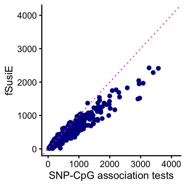
| Version | Author | Date |
|---|---|---|
| aece910 | Peter Carbonetto | 2025-03-24 |
One advantage of fSuSiE is that it is able to tell us which molecular features are affected by which SNPs, and therefore it provides a more coherent summary of how the SNPs affect methylation levels at a locus. To examine this quantitatively, we compare the number of affected CpGs per CS for fSuSiE to the number of affected CpGs per SNP from the association tests. The result is much fewer CSs and many more affected CpGs per CS:
x <- factor(methyl_cpg_assoc$variant_id)
cpgs_per_snp_assoc <- tapply(methyl_cpg_assoc$molecular_trait_id,x,
                             function (x) length(unique(x)))
rm(x)
cpgs_per_snp_fsusie <-
  with(methyl_cpg_fsusie,
       tapply(ID,cs,function (x) length(unique(x))))
pdat1 <- data.frame(x = cpgs_per_snp_assoc)
pdat2 <- data.frame(x = cpgs_per_snp_fsusie)
pdat1 <- subset(pdat1,x <= 25)
pdat2 <- subset(pdat2,x <= 250)
p1 <- ggplot(pdat1,aes(x = x)) +
  geom_histogram(color = "white",fill = "darkblue",bins = 25) +
  labs(x = "number of CpGs",y = "number of SNPs",
       title = "SNP-CpG association tests") +
  theme_cowplot(font_size = 10) +
  theme(plot.title = element_text(size = 10,face = "plain"))
p2 <- ggplot(pdat2,aes(x = x)) +
  geom_histogram(color = "white",fill = "darkblue",bins = 25) +
  labs(x = "number of CpGs",y = "number of CSs",title = "fSuSiE") +
  theme_cowplot(font_size = 10) +
  theme(plot.title = element_text(size = 10,face = "plain"))
plot_grid(p1,p2,nrow = 1,ncol = 2)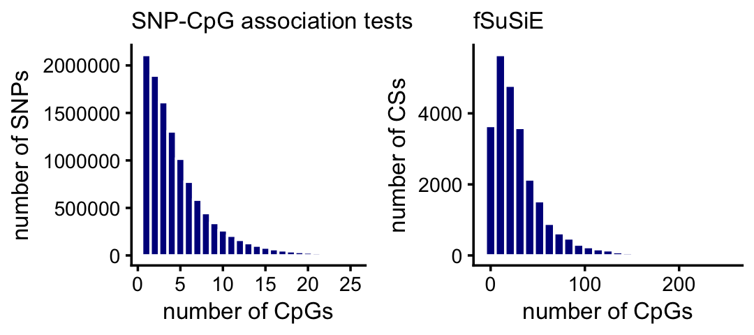
| Version | Author | Date |
|---|---|---|
| aece910 | Peter Carbonetto | 2025-03-24 |
A small proportion of the SNPs and CSs are not plotted because they have an unusually large number of CpGs:
mean(cpgs_per_snp_assoc > 25)
mean(cpgs_per_snp_fsusie > 250)
# [1] 0.01219941
# [1] 0.003076674
H3K27ac SNPs
Load the H3K27ac SNP results generated by SuSiE-topPC, fSuSiE and the SNP-peak association testing:
ha_peak_assoc_file <- "../outputs/ROSMAP_haQTL_qtl_snp_qval0.05.tsv.gz"
ha_snps_susie_file <- "../outputs/ROSMAP_haQTL_cs_snp_toppc1_annotation.tsv.gz"
ha_snps_fsusie_file <- "../outputs/ROSMAP_haQTL_cs_snp_annotation.tsv.gz"
ha_peak_assoc  <- read_enrichment_results(ha_peak_assoc_file,n = 8)
ha_snps_susie  <- read_enrichment_results(ha_snps_susie_file,n = 6)
ha_snps_fsusie <- read_enrichment_results(ha_snps_fsusie_file,n = 7)
ha_snps_susie$region <-
  sapply(strsplit(ha_snps_susie$cs,":",fixed = TRUE),"[[",2)
ha_snps_susie  <- transform(ha_snps_susie,
                            region = factor(region),
                            cs     = factor(cs),
                            pc     = factor(pc))
ha_snps_fsusie <- transform(ha_snps_fsusie,
                            cs     = factor(cs),
                            region = factor(region),
                            study  = factor(study))
There is no need to look at the TAD sizes because the same TADs were analyzed for both molecular traits, methylation and H3K27ac.
These histograms summarize the number of CSs per TAD:
pdat1 <- get_cs_vs_tad_size(ha_snps_susie)
pdat2 <- get_cs_vs_tad_size(ha_snps_fsusie)
pdat1 <- transform(pdat1,num_cs = factor(num_cs,1:20))
pdat2 <- transform(pdat2,num_cs = factor(num_cs,1:20))
p1 <- ggplot(pdat1,aes(x = num_cs)) +
  geom_histogram(stat = "count",color = "white",fill = "tomato") +
  scale_x_discrete(drop = FALSE) +
  labs(x = "number of CSs",y = "number of TADs",title = "SuSiE-topPC") +
  theme_cowplot(font_size = 10) +
  theme(plot.title = element_text(size = 10,face = "plain"))
p2 <- ggplot(pdat2,aes(x = num_cs)) +
  geom_histogram(stat = "count",color = "white",fill = "tomato") +
  scale_x_discrete(drop = FALSE) +
  labs(x = "number of CSs",y = "number of TADs",title = "fSuSiE") +
  theme_cowplot(font_size = 10) +
  theme(plot.title = element_text(size = 10,face = "plain"))
plot_grid(p1,p2,nrow = 1,ncol = 2)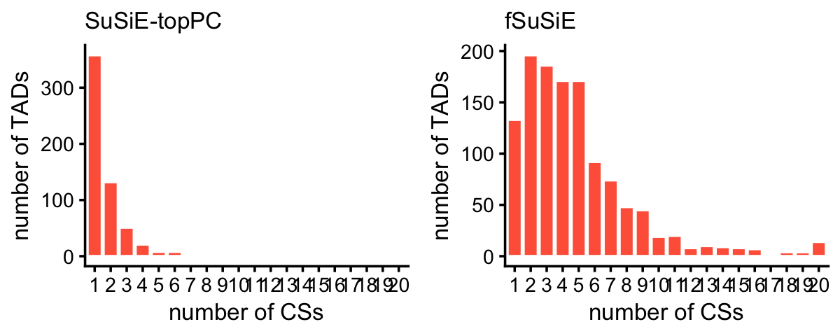
| Version | Author | Date |
|---|---|---|
| 71954f1 | Peter Carbonetto | 2025-03-20 |
Compare discovery of causal SNPs (number of CSs) in the SuSiE-topPC and fSuSiE analyses:
dat1 <- get_cs_vs_tad_size(ha_snps_susie)
dat2 <- get_cs_vs_tad_size(ha_snps_fsusie)
dat1 <- dat1[c(1,3)]
dat2 <- dat2[c(1,3)]
names(dat1) <- c("tad","num_cs_susie")
names(dat2) <- c("tad","num_cs_fsusie")
dat <- merge(dat1,dat2,all = TRUE)
rows <- which(is.na(dat$num_cs_susie))
dat[rows,"num_cs_susie"] <- 0
pdat <- melt(with(dat,table(num_cs_susie,num_cs_fsusie)))
rows <- which(pdat$value == 0)
pdat[rows,"value"] <- NA
p <- ggplot(pdat,aes(x = num_cs_susie,y = num_cs_fsusie,size = value)) +
  geom_point(color = "white",fill = "tomato",shape = 21) +
  geom_abline(intercept = 0,slope = 1,color = "black",linetype = "dotted") +
  scale_x_continuous(breaks = seq(0,20,2),limits = c(0,20)) +
  scale_y_continuous(breaks = seq(0,20,2),limits = c(0,20)) +
  scale_size(breaks = c(1,10,100)) +
  labs(x = "SuSiE-topPC",y = "fSuSiE",size = "number of TADs") +
  theme_cowplot(font_size = 10)
Compare the sizes of the CSs in the SuSiE-topPC and fSuSiE analyses:
bins <- c(0,1,2,5,10,20,Inf)
cs_size_susie  <- as.numeric(table(ha_snps_susie$cs))
cs_size_fsusie <- as.numeric(table(ha_snps_fsusie$cs))
cs_size_susie  <- cut(cs_size_susie,bins)
cs_size_fsusie <- cut(cs_size_fsusie,bins)
levels(cs_size_susie) <- bins[-1]
levels(cs_size_fsusie) <- bins[-1]
p1 <- ggplot(data.frame(cs_size = cs_size_susie),aes(x = cs_size)) +
  geom_histogram(stat = "count",color = "white",fill = "tomato",
                 width = 0.65) +
  labs(x = "CS size",y = "number of CSs",title = "SuSiE-topPC") +
  theme_cowplot(font_size = 10) +
  theme(plot.title = element_text(size = 10,face = "plain"))
p2 <- ggplot(data.frame(cs_size = cs_size_fsusie),aes(x = cs_size)) +
  geom_histogram(stat = "count",color = "white",fill = "tomato",
                 width = 0.65) +
  labs(x = "CS size",y = "number of CSs",title = "fSuSiE") +
  theme_cowplot(font_size = 10) +
  theme(plot.title = element_text(size = 10,face = "plain"))
plot_grid(p1,p2,nrow = 1,ncol = 2)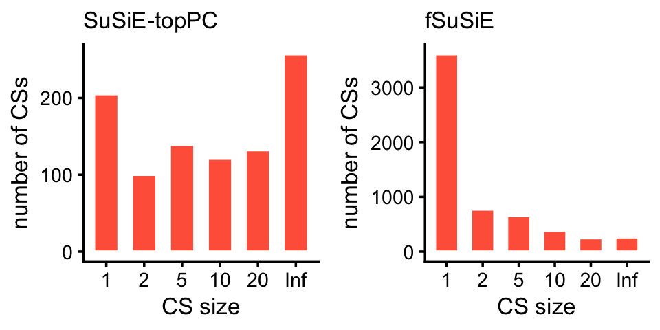
| Version | Author | Date |
|---|---|---|
| 71954f1 | Peter Carbonetto | 2025-03-20 |
We expect that the vast majority of the causal SNPs will be very close to the TSS. Let’s verify this empirically.
First, add a “min_dist_to_TSS” column to each set of results:
ha_snps_assoc  <- get_top_snp_per_location(ha_peak_assoc)
ha_snps_assoc  <- add_min_dist_to_tss(ha_snps_assoc,genes)
ha_snps_susie  <- add_min_dist_to_tss(ha_snps_susie,genes)
ha_snps_fsusie <- add_min_dist_to_tss(ha_snps_fsusie,genes)
This next code chunk computes the histogram for the TSS plot:
bin_size <- 5e4
bins <- c(-Inf,seq(-5e5,5.5e5,bin_size),Inf)
bins <- bins - bin_size/2
counts_assoc <- as.numeric(table(cut(ha_snps_assoc$min_dist_to_tss,bins)))
counts_susie <- tapply(ha_snps_susie$pip,
                       cut(ha_snps_susie$min_dist_to_tss,bins),
                       function (x) sum(x,na.rm = TRUE))
counts_fsusie <- tapply(ha_snps_fsusie$pip,
                        cut(ha_snps_fsusie$min_dist_to_tss,bins),
                        function (x) sum(x,na.rm = TRUE))
And now we can plot the result:
n <- length(bins)
i <- seq(2,n-2)
bin_centers   <- bins[i] + bin_size/2
counts_assoc  <- counts_assoc[i]
counts_susie  <- counts_susie[i]
counts_fsusie <- counts_fsusie[i]
counts_assoc  <- counts_assoc/sum(counts_assoc)
counts_susie  <- counts_susie/sum(counts_susie)
counts_fsusie <- counts_fsusie/sum(counts_fsusie)
pdat <- data.frame(method = rep(c("assoc","susie","fsusie"),
                                each = length(bin_centers)),
                   dist   = rep(bin_centers/1000,times = 3),
                   freq   = c(counts_assoc,counts_susie,counts_fsusie),
                   stringsAsFactors = TRUE)
p <- ggplot(pdat,aes(x = dist,y = freq,color = method)) +
  geom_line(linewidth = 0.5) +
  geom_point(size = 1) +
  scale_x_continuous(breaks = seq(-500,500,100),limits = c(-500,500)) +
  scale_y_continuous(breaks = seq(0,1,0.1)) +
  scale_color_manual(values = c("darkblue","darkorange","dodgerblue")) +
  labs(x = "distance to TSS (kb)",y = "proportion of SNPs") +
  theme_cowplot(font_size = 10)
print(p)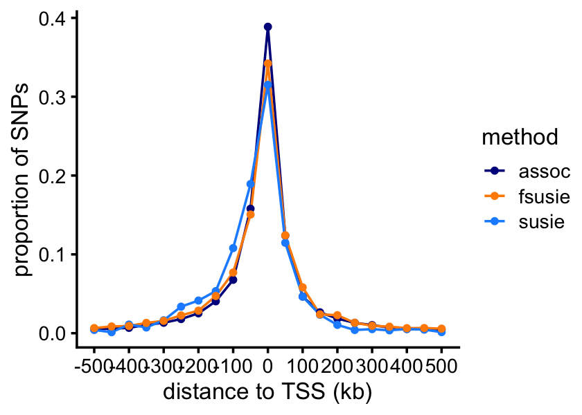
| Version | Author | Date |
|---|---|---|
| aece910 | Peter Carbonetto | 2025-03-24 |
Affected H3K27ac peaks
Now let’s turn to the recovery of affected H3K27ac peaks. First load the results generated by fSuSiE:
ha_peak_fsusie_file <-
  "../outputs/ROSMAP_haQTL_cs_effect_ha_peak_annotation.tsv.gz"
ha_peak_fsusie <- read_enrichment_results(ha_peak_fsusie_file,n = 9)
ha_peak_fsusie$region <-
  sapply(strsplit(ha_peak_fsusie$cs,":",fixed = TRUE),"[[",2)
ha_peak_fsusie <- transform(ha_peak_fsusie,
                            cs      = factor(cs),
                            region  = factor(region),
                            context = factor(context))
Count the number of affected peaks per TAD from the fSuSiE results:
ha_peaks_per_tad_fsusie <-
  with(ha_peak_fsusie,tapply(ID,region,function (x) length(unique(x))))
Next count the number of affected peaks per TAD from the SNP-peak association tests, using the functions defined above:
tads <- get_tad_info(levels(ha_peak_fsusie$region))
ha_peaks_per_tad_assoc <- count_features_per_tad(ha_peak_assoc,tads)
These two plots summarize the number of affected peaks per TAD:
ha_peaks_per_tad_assoc[ha_peaks_per_tad_assoc == 0] <- NA
ha_peaks_per_tad_fsusie[ha_peaks_per_tad_fsusie == 0] <- NA
pdat1 <- data.frame(x = ha_peaks_per_tad_assoc)
pdat2 <- data.frame(x = ha_peaks_per_tad_fsusie)
p1 <- ggplot(pdat1,aes(x = x)) +
  geom_histogram(color = "white",fill = "tomato",bins = 64) +
  xlim(0,200) +
  labs(x = "number of H3K27ac peaks",y = "number of TADs",
       title = "SNP-peak association tests") +
  theme_cowplot(font_size = 10) +
  theme(plot.title = element_text(size = 10,face = "plain"))
p2 <- ggplot(pdat2,aes(x = x)) +
  geom_histogram(color = "white",fill = "tomato",bins = 64) +
  xlim(0,200) +
  labs(x = "number of H3K27ac peaks",y = "number of TADs",title = "fSuSiE") +
  theme_cowplot(font_size = 10) +
  theme(plot.title = element_text(size = 10,face = "plain"))
plot_grid(p1,p2,nrow = 1,ncol = 2)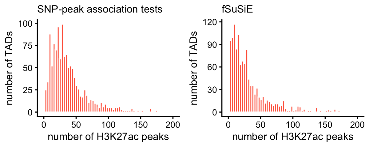
| Version | Author | Date |
|---|---|---|
| aece910 | Peter Carbonetto | 2025-03-24 |
A very small number of TADs have more than 200 affected peaks:
sum(ha_peaks_per_tad_assoc > 200,na.rm = TRUE)
sum(ha_peaks_per_tad_fsusie > 200,na.rm = TRUE)
# [1] 3
# [1] 6
This plot compares the number of affected H3K27ac peaks identified by fSuSiE and the SNP-peak association tests:
pdat <- data.frame(assoc  = ha_peaks_per_tad_assoc,
                   fsusie = ha_peaks_per_tad_fsusie)
ggplot(pdat,aes(x = assoc,y = fsusie)) +
  geom_point(color = "tomato") +
  geom_abline(intercept = 0,slope = 1,color = "magenta",linetype = "dotted") +
  labs(x = "SNP-peak association tests",y = "fSusiE") +
  xlim(0,200) +
  ylim(0,200) +
  theme_cowplot(font_size = 10)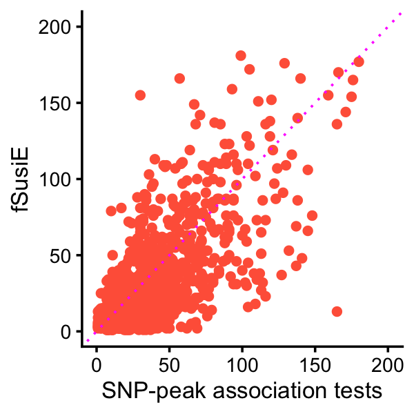
| Version | Author | Date |
|---|---|---|
| aece910 | Peter Carbonetto | 2025-03-24 |
These next two plots compare the number of affected peaks per CS for fSuSiE to the number of affected peaks per SNP from the association tests:
x <- factor(ha_peak_assoc$variant_id)
ha_peaks_per_snp_assoc <- tapply(ha_peak_assoc$molecular_trait_id,x,
                                 function (x) length(unique(x)))
rm(x)
ha_peaks_per_snp_fsusie <-
  with(ha_peak_fsusie,
       tapply(ID,cs,function (x) length(unique(x))))
pdat1 <- data.frame(x = ha_peaks_per_snp_assoc)
pdat2 <- data.frame(x = ha_peaks_per_snp_fsusie)
pdat1 <- subset(pdat1,x <= 10)
pdat2 <- subset(pdat2,x <= 40)
pdat1 <- transform(pdat1,x = factor(x))
p1 <- ggplot(pdat1,aes(x = x)) +
  geom_bar(color = "white",fill = "tomato") +
  labs(x = "number of H3K27ac peaks",y = "number of SNPs",
       title = "SNP-peak association tests") +
  theme_cowplot(font_size = 10) +
  theme(plot.title = element_text(size = 10,face = "plain"))
p2 <- ggplot(pdat2,aes(x = x)) +
  geom_histogram(color = "white",fill = "tomato",bins = 25) +
  labs(x = "number of H3K27ac peaks",y = "number of CSs",title = "fSuSiE") +
  theme_cowplot(font_size = 10) +
  theme(plot.title = element_text(size = 10,face = "plain"))
plot_grid(p1,p2,nrow = 1,ncol = 2)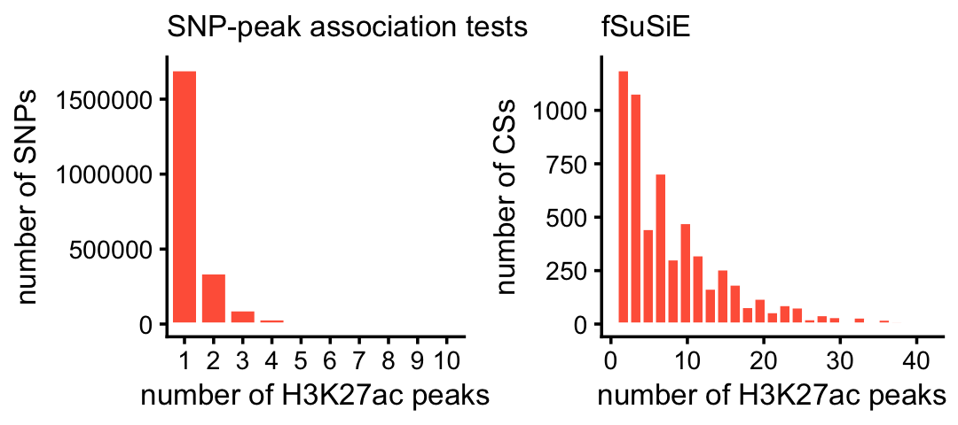
| Version | Author | Date |
|---|---|---|
| aece910 | Peter Carbonetto | 2025-03-24 |
A small proportion of the SNPs and CSs were not plotted because they had an unusually large number of affected peaks:
mean(ha_peaks_per_snp_assoc > 10)
mean(ha_peaks_per_snp_fsusie > 40)
# [1] 0.009820976
# [1] 0.007894285
sessionInfo()
# R version 4.3.3 (2024-02-29)
# Platform: aarch64-apple-darwin20 (64-bit)
# Running under: macOS Sonoma 14.7.1
#
# Matrix products: default
# BLAS:   /Library/Frameworks/R.framework/Versions/4.3-arm64/Resources/lib/libRblas.0.dylib
# LAPACK: /Library/Frameworks/R.framework/Versions/4.3-arm64/Resources/lib/libRlapack.dylib;  LAPACK version 3.11.0
#
# locale:
# [1] en_US.UTF-8/en_US.UTF-8/en_US.UTF-8/C/en_US.UTF-8/en_US.UTF-8
#
# time zone: America/Chicago
# tzcode source: internal
#
# attached base packages:
# [1] stats     graphics  grDevices utils     datasets  methods   base
#
# other attached packages:
# [1] cowplot_1.1.3     ggplot2_3.5.0     data.table_1.15.2
#
# loaded via a namespace (and not attached):
#  [1] sass_0.4.9        utf8_1.2.4        generics_0.1.3    stringi_1.8.3
#  [5] digest_0.6.34     magrittr_2.0.3    evaluate_0.23     grid_4.3.3
#  [9] fastmap_1.1.1     plyr_1.8.9        R.oo_1.26.0       rprojroot_2.0.4
# [13] workflowr_1.7.1   jsonlite_1.8.8    R.utils_2.12.3    whisker_0.4.1
# [17] promises_1.2.1    fansi_1.0.6       scales_1.3.0      textshaping_0.3.7
# [21] jquerylib_0.1.4   cli_3.6.4         rlang_1.1.5       R.methodsS3_1.8.2
# [25] munsell_0.5.0     withr_3.0.0       cachem_1.0.8      yaml_2.3.8
# [29] tools_4.3.3       reshape2_1.4.4    dplyr_1.1.4       colorspace_2.1-0
# [33] httpuv_1.6.14     vctrs_0.6.5       R6_2.5.1          lifecycle_1.0.4
# [37] git2r_0.33.0      stringr_1.5.1     fs_1.6.5          ragg_1.2.7
# [41] pkgconfig_2.0.3   pillar_1.9.0      bslib_0.6.1       later_1.3.2
# [45] gtable_0.3.4      glue_1.8.0        Rcpp_1.0.12       systemfonts_1.0.6
# [49] xfun_0.42         tibble_3.2.1      tidyselect_1.2.1  highr_0.10
# [53] knitr_1.45        farver_2.1.1      htmltools_0.5.8.1 labeling_0.4.3
# [57] rmarkdown_2.26    compiler_4.3.3