Examine ROSMAP H3K27ac fine-mapping results
William Denault, Hao Sun, Angjing Liu, Peter Carbonetto, Gao Wang
Last updated: 2025-05-13
Checks: 6 1
Knit directory:
fsusie-experiments/analysis/
This reproducible R Markdown analysis was created with workflowr (version 1.7.1). The Checks tab describes the reproducibility checks that were applied when the results were created. The Past versions tab lists the development history.
Great! Since the R Markdown file has been committed to the Git repository, you know the exact version of the code that produced these results.
Great job! The global environment was empty. Objects defined in the global environment can affect the analysis in your R Markdown file in unknown ways. For reproduciblity it’s best to always run the code in an empty environment.
The command set.seed(1) was run prior to running the
code in the R Markdown file. Setting a seed ensures that any results
that rely on randomness, e.g. subsampling or permutations, are
reproducible.
Great job! Recording the operating system, R version, and package versions is critical for reproducibility.
- flag-duplicated-cs
To ensure reproducibility of the results, delete the cache directory
rosmap_h3k27ac_cache and re-run the analysis. To have
workflowr automatically delete the cache directory prior to building the
file, set delete_cache = TRUE when running
wflow_build() or wflow_publish().
Great job! Using relative paths to the files within your workflowr project makes it easier to run your code on other machines.
Great! You are using Git for version control. Tracking code development and connecting the code version to the results is critical for reproducibility.
The results in this page were generated with repository version da54e8d. See the Past versions tab to see a history of the changes made to the R Markdown and HTML files.
Note that you need to be careful to ensure that all relevant files for
the analysis have been committed to Git prior to generating the results
(you can use wflow_publish or
wflow_git_commit). workflowr only checks the R Markdown
file, but you know if there are other scripts or data files that it
depends on. Below is the status of the Git repository when the results
were generated:
Untracked files:
    Untracked:  analysis/dist_hasnp_peak_cs1snp.pdf
    Untracked:  analysis/rosmap_h3k27ac_cache/
    Untracked:  analysis/rosmap_overview_cache/
    Untracked:  data/afreq.RData
    Untracked:  data/analysis_result/Fungen_xQTL.ENSG00000163808.cis_results_db.export.rds
    Untracked:  data/analysis_result/ROSMAP_haQTL.chr3_43915257_48413435.fsusie_mixture_normal_top_pc_weights.rds
    Untracked:  data/analysis_result/ROSMAP_mQTL.chr3_43915257_48413435.fsusie_mixture_normal_top_pc_weights.rds
    Untracked:  outputs/CASS4_all_effects.RData
    Untracked:  outputs/CASS4_obj.RData
    Untracked:  outputs/CD2AP_all_effects.RData
    Untracked:  outputs/CD2AP_obj.RData
    Untracked:  outputs/CR1_CR2_all_effects.RData
    Untracked:  outputs/CR1_CR2_obj.RData
    Untracked:  outputs/ROSMAP_DLPFC_mega_eQTL.cs_only.tsv.gz
    Untracked:  outputs/ROSMAP_DLPFC_pQTL.cs_only.tsv.gz
    Untracked:  outputs/ROSMAP_haQTL_cs_effect_ha_peak_annotation.tsv.gz
    Untracked:  outputs/ROSMAP_haQTL_cs_snp_annotation.tsv.gz
    Untracked:  outputs/ROSMAP_haQTL_cs_snp_toppc1_annotation.tsv.gz
    Untracked:  outputs/ROSMAP_haQTL_qtl_snp_qval0.05.tsv.gz
    Untracked:  outputs/ROSMAP_haQTL_qtl_snp_qval0.05_annotation.tsv.gz
    Untracked:  outputs/ROSMAP_mQTL_cs_effect_cpg_annotation.tsv.gz
    Untracked:  outputs/ROSMAP_mQTL_cs_snp_annotation.tsv.gz
    Untracked:  outputs/ROSMAP_mQTL_cs_snp_toppc1_annotation.tsv.gz
    Untracked:  outputs/ROSMAP_mQTL_qtl_snp_qval0.05.tsv.gz
    Untracked:  outputs/ROSMAP_mQTL_qtl_snp_qval0.05_annotation.tsv.gz
Note that any generated files, e.g. HTML, png, CSS, etc., are not included in this status report because it is ok for generated content to have uncommitted changes.
These are the previous versions of the repository in which changes were
made to the R Markdown (analysis/rosmap_h3k27ac.Rmd) and
HTML (docs/rosmap_h3k27ac.html) files. If you’ve configured
a remote Git repository (see ?wflow_git_remote), click on
the hyperlinks in the table below to view the files as they were in that
past version.
| File | Version | Author | Date | Message |
|---|---|---|---|---|
| Rmd | da54e8d | Peter Carbonetto | 2025-05-13 | A few fixes to rosmap_h3k27ac.Rmd. |
| Rmd | 5d9c3bd | Peter Carbonetto | 2025-05-13 | Small fix to rosmap_overview.Rmd. |
| Rmd | 392f166 | Peter Carbonetto | 2025-05-13 | Added haSNP-peak histogram to the rosmap_h3k27ac analysis. |
| Rmd | 6ac1ef3 | Peter Carbonetto | 2025-05-13 | Fixed a bug in rosmap_h3k27ac.Rmd. |
| Rmd | 09385ee | Peter Carbonetto | 2025-05-13 | Working on adding affected peak results to the rosmap_h3k27ac analysis; also added a step to remove duplicated CSs from peak-level results for fSuSiE as well as a MAF filtering step for the SNP-peak association testing results. |
| Rmd | c38f32b | Peter Carbonetto | 2025-05-13 | Applied MAF filter to snps_assoc in rosmap_h3k27ac analysis. |
| Rmd | 69dcefa | Peter Carbonetto | 2025-05-13 | Added steps to the rosmap_h3k27ac analysis to load the peak-level results and apply the MAF filter to them. |
| Rmd | 890a515 | Peter Carbonetto | 2025-05-13 | Added tables to the rosmap_h3k27ac analysis showing the distribution of PIPs in the 1-SNP CSs. |
| html | 75fcda1 | Peter Carbonetto | 2025-05-13 | Ran wflow_publish("rosmap_h3k27ac.Rmd"). |
| Rmd | acd259e | Peter Carbonetto | 2025-05-13 | Added TSS plot to rosmap_h3k27ac analysis. |
| Rmd | 1c5ff9e | Peter Carbonetto | 2025-05-13 | Added step to remove duplicate CSs and added CS size histograms to rosmap_h3k27ac analysis. |
| Rmd | 9a0d3ab | Peter Carbonetto | 2025-05-13 | Added plots to rosmap_h3k27ac analysis comparing discovery of CSs in TADs. |
| Rmd | e6480b7 | Peter Carbonetto | 2025-05-13 | Added steps to rosmap_h3k27ac analysis to load gene data, allele frequency data, and fine-mapping results. |
| Rmd | ed237c6 | Peter Carbonetto | 2025-05-13 | Started new analysis rosmap_h3k27ac.Rmd. |
Note: If you would like to run this analysis on your computer, you will first need to download the fine-mapping outputs. They can be downloaded from here. Once you have downloaded the files, copy each file to the “data” or “outputs” subdirectory.
Load some packages and custom functions used in the code below:
library(data.table)
library(dplyr)
library(ggplot2)
library(cowplot)
source("../code/rosmap_functions_more.R")
Load the gene annotations used in some of the analyses below.
gene_file <-
  file.path("../data/genome_annotations",
    "Homo_sapiens.GRCh38.103.chr.reformatted.collapse_only.gene.gtf.gz")
genes <- get_gene_annotations(gene_file)
Load the allele frequencies computed by PLINK:
load("../data/afreq.RData")Load the H3K27ac SNP results generated by SuSiE-topPC, fSuSiE and the SNP-peak association testing:
assoc_file       <- "../outputs/ROSMAP_haQTL_qtl_snp_qval0.05.tsv.gz"
snps_susie_file  <- "../outputs/ROSMAP_haQTL_cs_snp_toppc1_annotation.tsv.gz"
snps_fsusie_file <- "../outputs/ROSMAP_haQTL_cs_snp_annotation.tsv.gz"
assoc       <- read_enrichment_results(assoc_file,n = 8)
snps_susie  <- read_enrichment_results(snps_susie_file,n = 6)
snps_fsusie <- read_enrichment_results(snps_fsusie_file,n = 7)
snps_susie  <- snps_susie[1:6]
snps_fsusie <- snps_fsusie[1:7]
snps_susie$region <-
  sapply(strsplit(snps_susie$cs,":",fixed = TRUE),"[[",2)
snps_susie  <- transform(snps_susie,
                         region = factor(region),
                         cs     = factor(cs),
                         pc     = factor(pc))
snps_fsusie <- transform(snps_fsusie,
                         cs     = factor(cs),
                         region = factor(region),
                         study  = factor(study))
Add the allele frequencies to the H3K27ac fine-mapping results:
ids  <- with(snps_susie,paste(chr,pos,sep = "_"))
rows <- match(ids,afreq$id)
snps_susie$maf <- afreq[rows,"maf"]
ids  <- with(snps_fsusie,paste(chr,pos,sep = "_"))
rows <- match(ids,afreq$id)
snps_fsusie$maf <- afreq[rows,"maf"]
Also load the peak-level results generated by fSuSiE:
peaks_fsusie_file <-
  "../outputs/ROSMAP_haQTL_cs_effect_ha_peak_annotation.tsv.gz"
peaks_fsusie <- read_enrichment_results(peaks_fsusie_file,n = 9)
peaks_fsusie <- peaks_fsusie[1:9]
peaks_fsusie$region <-
  sapply(strsplit(peaks_fsusie$cs,":",fixed = TRUE),"[[",2)
peaks_fsusie <- transform(peaks_fsusie,
                          cs      = factor(cs),
                          region  = factor(region),
                          context = factor(context))
Keep only CSs if the MAF of the sentinel SNP is >5%:
keep        <- tapply(snps_susie[c("pip","maf")],snps_susie$cs,
                      function (x) x[which.max(x$pip),"maf"] >= 0.05)
keep_cs     <- names(which(keep))
snps_susie  <- subset(snps_susie,is.element(cs,keep_cs))
snps_susie  <- transform(snps_susie,
                         region = factor(region),
                         cs     = factor(cs))
keep        <- tapply(snps_fsusie[c("pip","maf")],snps_fsusie$cs,
                      function (x) x[which.max(x$pip),"maf"] >= 0.05)
keep_cs     <- names(which(keep))
snps_fsusie <- subset(snps_fsusie,is.element(cs,keep_cs))
snps_fsusie <- transform(snps_fsusie,
                         region = factor(region),
                         cs     = factor(cs))
Apply this same MAF filter to the SNP-peak association tests and the fSuSiE peak-level results:
ids          <- with(assoc,paste(chr,pos,sep = "_"))
rows         <- match(ids,afreq$id)
assoc$maf    <- afreq[rows,"maf"]
assoc        <- subset(assoc,maf >= 0.05)
peaks_fsusie <- subset(peaks_fsusie,is.element(cs,keep_cs))
peaks_fsusie <- transform(peaks_fsusie,
                          region = factor(region),
                          cs     = factor(cs))
There is no need to look at the TAD sizes here because the same TADs were analyzed for both of the molecular traits (methylation and H3K27ac).
These histograms summarize the number of CSs per TAD:
pdat1 <- get_cs_vs_tad_size(snps_susie)
pdat2 <- get_cs_vs_tad_size(snps_fsusie)
pdat1 <- transform(pdat1,num_cs = factor(num_cs,1:20))
pdat2 <- transform(pdat2,num_cs = factor(num_cs,1:20))
p1 <- ggplot(pdat1,aes(x = num_cs)) +
  geom_histogram(stat = "count",color = "white",fill = "tomato") +
  scale_x_discrete(drop = FALSE) +
  labs(x = "number of CSs",y = "number of TADs",title = "SuSiE-topPC") +
  theme_cowplot(font_size = 10) +
  theme(plot.title = element_text(size = 10,face = "plain"))
p2 <- ggplot(pdat2,aes(x = num_cs)) +
  geom_histogram(stat = "count",color = "white",fill = "tomato") +
  scale_x_discrete(drop = FALSE) +
  labs(x = "number of CSs",y = "number of TADs",title = "fSuSiE") +
  theme_cowplot(font_size = 10) +
  theme(plot.title = element_text(size = 10,face = "plain"))
plot_grid(p1,p2,nrow = 1,ncol = 2)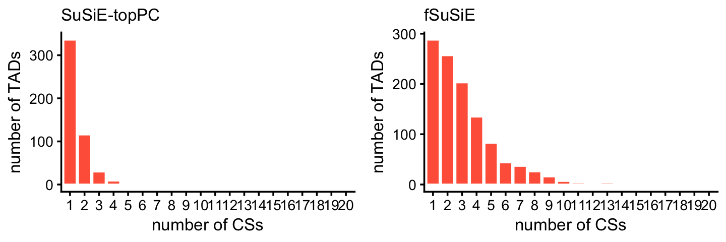
| Version | Author | Date |
|---|---|---|
| 75fcda1 | Peter Carbonetto | 2025-05-13 |
Compare discovery of causal SNPs (number of CSs) in the SuSiE-topPC and fSuSiE analyses:
dat1 <- get_cs_vs_tad_size(snps_susie)
dat2 <- get_cs_vs_tad_size(snps_fsusie)
dat1 <- dat1[c(1,3)]
dat2 <- dat2[c(1,3)]
names(dat1) <- c("tad","num_cs_susie")
names(dat2) <- c("tad","num_cs_fsusie")
dat <- merge(dat1,dat2,all = TRUE)
rows <- which(is.na(dat$num_cs_susie))
dat[rows,"num_cs_susie"] <- 0
pdat <- melt(with(dat,table(num_cs_susie,num_cs_fsusie)))
rows <- which(pdat$value == 0)
pdat[rows,"value"] <- NA
p <- ggplot(pdat,aes(x = num_cs_susie,y = num_cs_fsusie,size = value)) +
  geom_point(color = "white",fill = "tomato",shape = 21) +
  geom_abline(intercept = 0,slope = 1,color = "black",linetype = "dotted") +
  scale_x_continuous(breaks = seq(0,20,2),limits = c(0,20)) +
  scale_y_continuous(breaks = seq(0,20,2),limits = c(0,20)) +
  scale_size(breaks = c(1,10,100)) +
  labs(x = "SuSiE-topPC",y = "fSuSiE",size = "number of TADs") +
  theme_cowplot(font_size = 10)
print(p)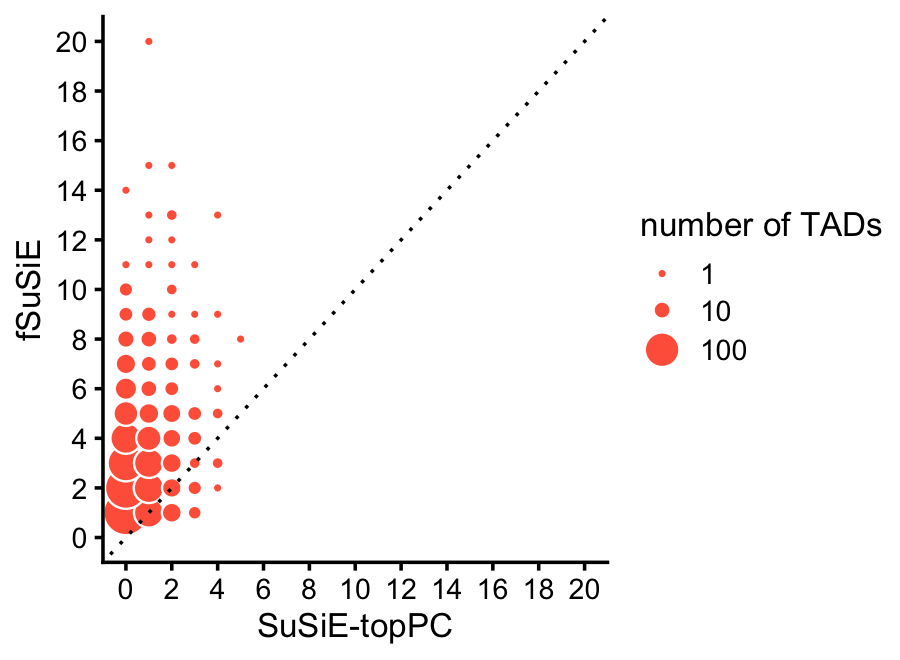
| Version | Author | Date |
|---|---|---|
| 75fcda1 | Peter Carbonetto | 2025-05-13 |
Flag the “duplicate” CSs:
root_cs_susie  <- create_cs_maps(snps_susie)$root
root_cs_fsusie <- create_cs_maps(snps_fsusie)$root
Warning: The above code chunk cached its results, but
it won’t be re-run if previous chunks it depends on are updated. If you
need to use caching, it is highly recommended to also set
knitr::opts_chunk$set(autodep = TRUE) at the top of the
file (in a chunk that is not cached). Alternatively, you can customize
the option dependson for each individual chunk that is
cached. Using either autodep or dependson will
remove this warning. See the
knitr cache options for more details.
Then remove the duplicate CSs:
snps_susie  <- subset(snps_susie,is.element(cs,root_cs_susie))
snps_fsusie <- subset(snps_fsusie,is.element(cs,root_cs_fsusie))
snps_susie  <- transform(snps_susie,cs = factor(cs))
snps_fsusie <- transform(snps_fsusie,cs = factor(cs))
Also remove the duplicate CSs from the fSuSiE peak-level results:
nodup_cs     <- levels(snps_fsusie$cs)
peaks_fsusie <- subset(peaks_fsusie,is.element(cs,nodup_cs))
peaks_fsusie <- transform(peaks_fsusie,cs = factor(cs))
Compare the sizes of the CSs in the SuSiE-topPC and fSuSiE analyses:
bins <- c(0,1,2,5,10,20,Inf)
cs_size_susie  <- as.numeric(table(snps_susie$cs))
cs_size_fsusie <- as.numeric(table(snps_fsusie$cs))
cs_size_susie  <- cut(cs_size_susie,bins)
cs_size_fsusie <- cut(cs_size_fsusie,bins)
levels(cs_size_susie) <- bins[-1]
levels(cs_size_fsusie) <- bins[-1]
p1 <- ggplot(data.frame(cs_size = cs_size_susie),aes(x = cs_size)) +
  geom_histogram(stat = "count",color = "white",fill = "tomato",
                 width = 0.65) +
  labs(x = "CS size",y = "number of CSs",title = "SuSiE-topPC") +
  theme_cowplot(font_size = 10) +
  theme(plot.title = element_text(size = 10,face = "plain"))
p2 <- ggplot(data.frame(cs_size = cs_size_fsusie),aes(x = cs_size)) +
  geom_histogram(stat = "count",color = "white",fill = "tomato",
                 width = 0.65) +
  labs(x = "CS size",y = "number of CSs",title = "fSuSiE") +
  theme_cowplot(font_size = 10) +
  theme(plot.title = element_text(size = 10,face = "plain"))
plot_grid(p1,p2,nrow = 1,ncol = 2)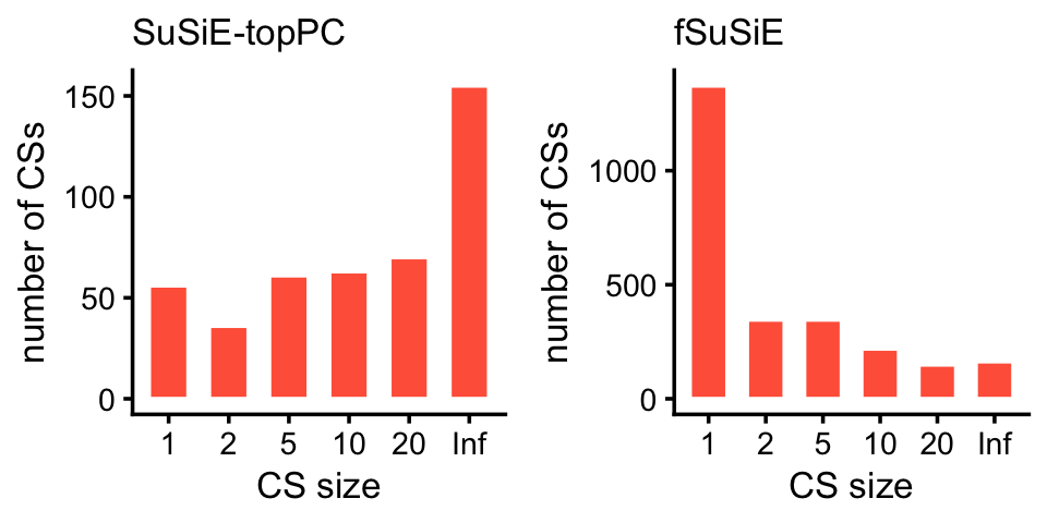
| Version | Author | Date |
|---|---|---|
| 75fcda1 | Peter Carbonetto | 2025-05-13 |
Here are the exact numbers:
table(cs_size_susie)
table(cs_size_fsusie)
# cs_size_susie
#   1   2   5  10  20 Inf
#  56  36  61  63  70 155
# cs_size_fsusie
#    1    2    5   10   20  Inf
# 1372  346  346  219  149  163
We expect that the vast majority of the causal SNPs will be very close to the TSS. Let’s verify this empirically.
First, add a “min_dist_to_TSS” column to each set of results:
snps_assoc  <- get_top_snp_per_location(assoc)
snps_assoc  <- add_min_dist_to_tss(snps_assoc,genes)
snps_susie  <- add_min_dist_to_tss(snps_susie,genes)
snps_fsusie <- add_min_dist_to_tss(snps_fsusie,genes)
This next code chunk computes the histogram for the TSS plot:
bin_size <- 5e4
bins <- c(-Inf,seq(-5e5,5.5e5,bin_size),Inf)
bins <- bins - bin_size/2
counts_assoc <- as.numeric(table(cut(snps_assoc$min_dist_to_tss,bins)))
counts_susie <- tapply(snps_susie$pip,
                       cut(snps_susie$min_dist_to_tss,bins),
                       function (x) sum(x,na.rm = TRUE))
counts_fsusie <- tapply(snps_fsusie$pip,
                        cut(snps_fsusie$min_dist_to_tss,bins),
                        function (x) sum(x,na.rm = TRUE))
And now we can plot the result:
n <- length(bins)
i <- seq(2,n-2)
bin_centers   <- bins[i] + bin_size/2
counts_assoc  <- counts_assoc[i]
counts_susie  <- counts_susie[i]
counts_fsusie <- counts_fsusie[i]
counts_assoc  <- counts_assoc/sum(counts_assoc)
counts_susie  <- counts_susie/sum(counts_susie)
counts_fsusie <- counts_fsusie/sum(counts_fsusie)
pdat <- data.frame(method = rep(c("assoc","susie","fsusie"),
                                each = length(bin_centers)),
                   dist   = rep(bin_centers/1000,times = 3),
                   freq   = c(counts_assoc,counts_susie,counts_fsusie),
                   stringsAsFactors = TRUE)
p <- ggplot(pdat,aes(x = dist,y = freq,color = method)) +
  geom_line(linewidth = 0.5) +
  geom_point(size = 1) +
  scale_x_continuous(breaks = seq(-500,500,100),limits = c(-500,500)) +
  scale_y_continuous(breaks = seq(0,1,0.1)) +
  scale_color_manual(values = c("darkblue","darkorange","dodgerblue")) +
  labs(x = "distance to TSS (kb)",y = "proportion of SNPs") +
  theme_cowplot(font_size = 10)
print(p)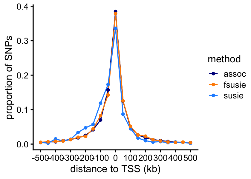
| Version | Author | Date |
|---|---|---|
| 75fcda1 | Peter Carbonetto | 2025-05-13 |
Now let’s look closely at the 1-SNP CSs.
cs1snp_susie  <- table(snps_susie$cs)
cs1snp_susie  <- names(cs1snp_susie)[cs1snp_susie == 1]
cs1snp_susie  <- subset(snps_susie,is.element(cs,cs1snp_susie))
cs1snp_fsusie <- table(snps_fsusie$cs)
cs1snp_fsusie <- names(cs1snp_fsusie)[cs1snp_fsusie == 1]
cs1snp_fsusie <- subset(snps_fsusie,is.element(cs,cs1snp_fsusie))
Many of the PIPs in the 1-SNP CSs are 1 or very close to 1:
table(cut(1 - cs1snp_susie$pip,c(0,0.0001,0.001,0.01,1)))
table(cut(1 - cs1snp_fsusie$pip,c(0,0.0001,0.001,0.01,1)))
#
#     (0,0.0001] (0.0001,0.001]   (0.001,0.01]       (0.01,1]
#             17              6             16             12
#
#     (0,0.0001] (0.0001,0.001]   (0.001,0.01]       (0.01,1]
#            558            179            179            237
This plot shows the distribution of the distances between the haSNP (in the 1-SNP CS) and the nearest H3K27ac peak affected by that SNP:
Count the number of affected peaks per TAD from the fSuSiE results:
peaks_per_tad_fsusie <-
  with(peaks_fsusie,tapply(ID,region,function (x) length(unique(x))))
Counting the number of H3K27ac peaks per TAD from the SNP-peak association tests is a little more complicated because the peaks were not assigned to TADs in the results.
tads <- get_tad_info(levels(peaks_fsusie$region))
peaks_per_tad_assoc <- count_features_per_tad(assoc,tads)
These two plots summarize the number of affected peaks per TAD:
peaks_per_tad_assoc[peaks_per_tad_assoc == 0] <- NA
peaks_per_tad_fsusie[peaks_per_tad_fsusie == 0] <- NA
pdat1 <- data.frame(x = peaks_per_tad_assoc)
pdat2 <- data.frame(x = peaks_per_tad_fsusie)
p1 <- ggplot(pdat1,aes(x = x)) +
  geom_histogram(color = "white",fill = "tomato",bins = 64) +
  xlim(0,100) +
  labs(x = "number of H3K27ac peaks",y = "number of TADs",
       title = "SNP-peak association tests") +
  theme_cowplot(font_size = 10) +
  theme(plot.title = element_text(size = 10,face = "plain"))
p2 <- ggplot(pdat2,aes(x = x)) +
  geom_histogram(color = "white",fill = "tomato",bins = 64) +
  xlim(0,100) +
  labs(x = "number of H3K27ac peaks",y = "number of TADs",title = "fSuSiE") +
  theme_cowplot(font_size = 10) +
  theme(plot.title = element_text(size = 10,face = "plain"))
plot_grid(p1,p2,nrow = 1,ncol = 2)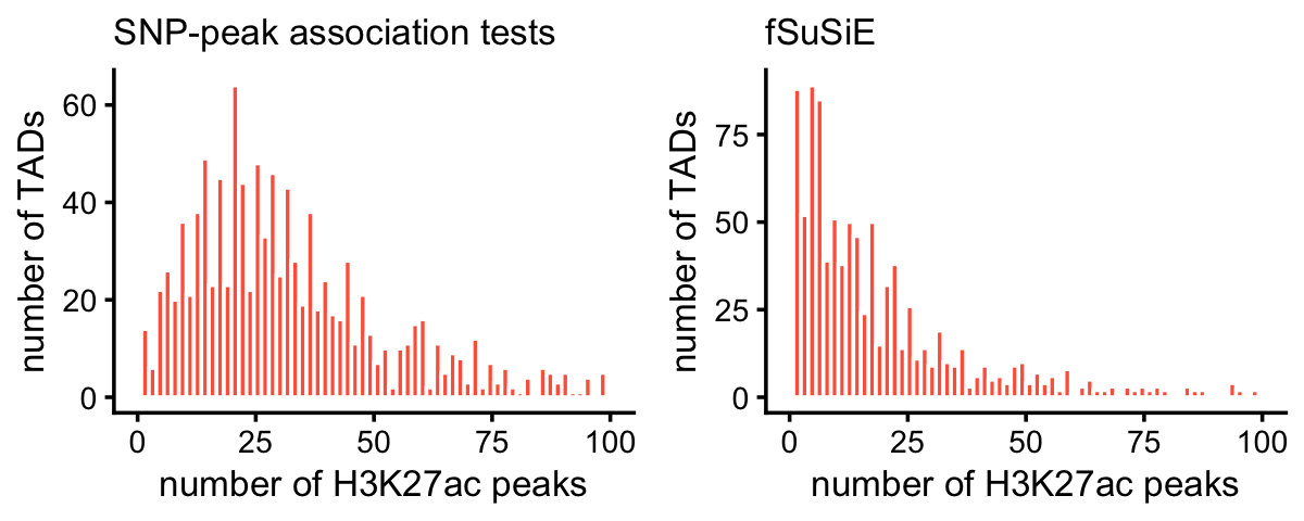
A very small number of TADs have more than 100 affected peaks:
mean(peaks_per_tad_assoc > 100,na.rm = TRUE)
mean(peaks_per_tad_fsusie > 100,na.rm = TRUE)
# [1] 0.04343891
# [1] 0.02446483
This plot compares the number of affected H3K27ac peaks per TAD identified by fSuSiE and by the SNP-peak association tests:
pdat <- data.frame(assoc  = peaks_per_tad_assoc,
                   fsusie = peaks_per_tad_fsusie)
p <- ggplot(pdat,aes(x = assoc,y = fsusie)) +
  geom_point(color = "tomato") +
  geom_abline(intercept = 0,slope = 1,color = "black",linetype = "dotted") +
  labs(x = "SNP-peak association tests",y = "fSusiE") +
  xlim(0,200) +
  ylim(0,200) +
  theme_cowplot(font_size = 10)
print(p)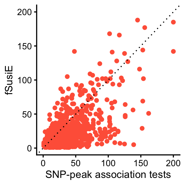
These next two plots compare the number of affected peaks per CS for fSuSiE to the number of affected peaks per SNP from the association tests:
x <- factor(assoc$variant_id)
peaks_per_snp_assoc <- tapply(assoc$molecular_trait_id,x,
                              function (x) length(unique(x)))
rm(x)
peaks_per_snp_fsusie <-
  with(peaks_fsusie,tapply(ID,cs,function (x) length(unique(x))))
pdat1 <- data.frame(x = peaks_per_snp_assoc)
pdat2 <- data.frame(x = peaks_per_snp_fsusie)
pdat1 <- subset(pdat1,x <= 10)
pdat2 <- subset(pdat2,x <= 40)
pdat1 <- transform(pdat1,x = factor(x))
p1 <- ggplot(pdat1,aes(x = x)) +
  geom_bar(color = "white",fill = "tomato") +
  labs(x = "number of H3K27ac peaks",y = "number of SNPs",
       title = "SNP-peak association tests") +
  theme_cowplot(font_size = 10) +
  theme(plot.title = element_text(size = 10,face = "plain"))
p2 <- ggplot(pdat2,aes(x = x)) +
  geom_histogram(color = "white",fill = "tomato",bins = 25) +
  labs(x = "number of H3K27ac peaks",y = "number of CSs",title = "fSuSiE") +
  theme_cowplot(font_size = 10) +
  theme(plot.title = element_text(size = 10,face = "plain"))
plot_grid(p1,p2,nrow = 1,ncol = 2)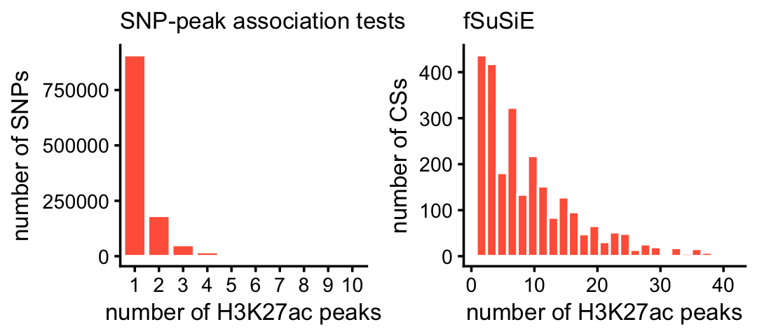
A small proportion of the SNPs and CSs were not plotted because they had an unusually large number of affected peaks:
mean(peaks_per_snp_assoc > 10)
mean(peaks_per_snp_fsusie > 40)
# [1] 0.009381663
# [1] 0.008607199
Finally, this plot shows the distribution of the distances between the haSNP (in a 1-SNP CS) and the nearest peak affected by that SNP:
peaks_fsusie_cs1snp <- subset(peaks_fsusie,
                              is.element(cs,cs1snp_fsusie$cs))
rows <- match(peaks_fsusie_cs1snp$cs,cs1snp_fsusie$cs)
peaks_fsusie_cs1snp$variant_pos <- cs1snp_fsusie[rows,"pos"]
peaks_fsusie_cs1snp <-
  transform(peaks_fsusie_cs1snp,
            cs   = factor(cs),
            dist = (peak_start + peak_end)/2 - variant_pos)
pdat <- tapply(peaks_fsusie_cs1snp$dist,peaks_fsusie_cs1snp$cs,
               function (x) {
                 i <- which.min(abs(x))
                 return(x[i])
               })
pdat <- data.frame(dist = pdat/1e6)
p <- ggplot(subset(pdat,abs(dist) < 2),aes(x = dist)) +
  geom_histogram(bins = 128,color = "tomato",fill = "tomato") +
  scale_y_continuous(breaks = seq(0,500,100)) +
  labs(x = "peak - haSNP position (Mb)",
       y = "number of haSNPs") +
  theme_cowplot(font_size = 10)
print(p)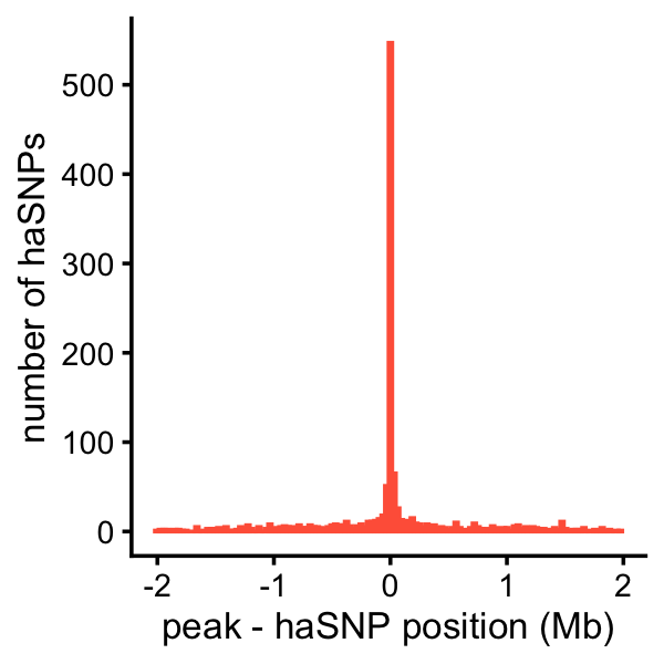
table(abs(pdat$dist) < 2)
#
# FALSE  TRUE
#   112  1235
sessionInfo()
# R version 4.3.3 (2024-02-29)
# Platform: aarch64-apple-darwin20 (64-bit)
# Running under: macOS 15.4.1
#
# Matrix products: default
# BLAS:   /Library/Frameworks/R.framework/Versions/4.3-arm64/Resources/lib/libRblas.0.dylib
# LAPACK: /Library/Frameworks/R.framework/Versions/4.3-arm64/Resources/lib/libRlapack.dylib;  LAPACK version 3.11.0
#
# locale:
# [1] en_US.UTF-8/en_US.UTF-8/en_US.UTF-8/C/en_US.UTF-8/en_US.UTF-8
#
# time zone: America/Chicago
# tzcode source: internal
#
# attached base packages:
# [1] stats     graphics  grDevices utils     datasets  methods   base
#
# other attached packages:
# [1] cowplot_1.1.3     ggplot2_3.5.0     dplyr_1.1.4       data.table_1.15.2
#
# loaded via a namespace (and not attached):
#  [1] sass_0.4.9        utf8_1.2.4        generics_0.1.3    stringi_1.8.3
#  [5] digest_0.6.34     magrittr_2.0.3    evaluate_1.0.3    grid_4.3.3
#  [9] fastmap_1.1.1     plyr_1.8.9        R.oo_1.26.0       rprojroot_2.0.4
# [13] workflowr_1.7.1   jsonlite_1.8.8    R.utils_2.12.3    whisker_0.4.1
# [17] promises_1.2.1    fansi_1.0.6       scales_1.3.0      textshaping_0.3.7
# [21] jquerylib_0.1.4   cli_3.6.4         rlang_1.1.5       R.methodsS3_1.8.2
# [25] munsell_0.5.0     withr_3.0.2       cachem_1.0.8      yaml_2.3.8
# [29] tools_4.3.3       reshape2_1.4.4    colorspace_2.1-0  httpuv_1.6.14
# [33] vctrs_0.6.5       R6_2.5.1          lifecycle_1.0.4   git2r_0.33.0
# [37] stringr_1.5.1     fs_1.6.5          ragg_1.2.7        pkgconfig_2.0.3
# [41] pillar_1.9.0      bslib_0.6.1       later_1.3.2       gtable_0.3.4
# [45] glue_1.8.0        Rcpp_1.0.12       systemfonts_1.0.6 xfun_0.42
# [49] tibble_3.2.1      tidyselect_1.2.1  highr_0.10        knitr_1.45
# [53] farver_2.1.1      htmltools_0.5.8.1 rmarkdown_2.26    labeling_0.4.3
# [57] compiler_4.3.3