Clustering Cusanovich et al (2018) data using topic proportions with K = 13 topics
Kaixuan Luo
Last updated: 2020-12-02
Checks: 7 0
Knit directory: scATACseq-topics/
This reproducible R Markdown analysis was created with workflowr (version 1.6.2). The Checks tab describes the reproducibility checks that were applied when the results were created. The Past versions tab lists the development history.
Great! Since the R Markdown file has been committed to the Git repository, you know the exact version of the code that produced these results.
Great job! The global environment was empty. Objects defined in the global environment can affect the analysis in your R Markdown file in unknown ways. For reproduciblity it's best to always run the code in an empty environment.
The command set.seed(20200729) was run prior to running the code in the R Markdown file. Setting a seed ensures that any results that rely on randomness, e.g. subsampling or permutations, are reproducible.
Great job! Recording the operating system, R version, and package versions is critical for reproducibility.
Nice! There were no cached chunks for this analysis, so you can be confident that you successfully produced the results during this run.
Great job! Using relative paths to the files within your workflowr project makes it easier to run your code on other machines.
Great! You are using Git for version control. Tracking code development and connecting the code version to the results is critical for reproducibility.
The results in this page were generated with repository version 06efc2b. See the Past versions tab to see a history of the changes made to the R Markdown and HTML files.
Note that you need to be careful to ensure that all relevant files for the analysis have been committed to Git prior to generating the results (you can use wflow_publish or wflow_git_commit). workflowr only checks the R Markdown file, but you know if there are other scripts or data files that it depends on. Below is the status of the Git repository when the results were generated:
Ignored files:
    Ignored:    .Rhistory
    Ignored:    .Rproj.user/

Untracked files:
    Untracked:  analysis/clusters_pca_structure_Cusanovich2018.Rmd
    Untracked:  analysis/motif_analysis_Buenrostro2018_chomVAR_scPeaks.Rmd
    Untracked:  analysis/process_data_Buenrostro2018_Chen2019.Rmd
    Untracked:  buenrostro2018.RData
    Untracked:  output/clustering-Cusanovich2018.rds
    Untracked:  scripts/fit_all_models_Buenrostro_2018_chromVar_scPeaks_filtered.sbatch

Unstaged changes:
    Modified:   analysis/cisTopic_Buenrostro2018_chomVAR_scPeaks.Rmd
    Modified:   analysis/plots_Lareau2019_bonemarrow.Rmd
    Modified:   analysis/process_data_Buenrostro2018.Rmd
    Modified:   code/motif_analysis.R
    Modified:   code/plots.R
    Modified:   scripts/fit_all_models_Buenrostro_2018.sbatch
Note that any generated files, e.g. HTML, png, CSS, etc., are not included in this status report because it is ok for generated content to have uncommitted changes.
These are the previous versions of the repository in which changes were made to the R Markdown (analysis/clusters_Cusanovich2018_k13.Rmd) and HTML (docs/clusters_Cusanovich2018_k13.html) files. If you've configured a remote Git repository (see ?wflow_git_remote), click on the hyperlinks in the table below to view the files as they were in that past version.
| File | Version | Author | Date | Message |
|---|---|---|---|---|
| Rmd | 06efc2b | kevinlkx | 2020-12-02 | zoom into a few clusters |
| html | 96392bf | kevinlkx | 2020-12-02 | Build site. |
| Rmd | 8db261b | kevinlkx | 2020-12-02 | wflow_publish("analysis/clusters_Cusanovich2018_k13.Rmd") |
| html | deead06 | kevinlkx | 2020-12-01 | Build site. |
| Rmd | 2af43a8 | kevinlkx | 2020-12-01 | update tissue colors |
| html | 06b9bc9 | kevinlkx | 2020-12-01 | Build site. |
| Rmd | bc7e770 | kevinlkx | 2020-12-01 | update tissue colors |
| html | 6c97fa9 | kevinlkx | 2020-12-01 | Build site. |
| Rmd | ab321de | kevinlkx | 2020-12-01 | refine kmeans clusters and add cell label distributions |
| html | e57dfd4 | kevinlkx | 2020-10-21 | Build site. |
| Rmd | a88649d | kevinlkx | 2020-10-21 | wflow_publish("analysis/clusters_Cusanovich2018_k13.Rmd") |
| Rmd | 137c252 | kevinlkx | 2020-10-21 | set toc = yes |
| html | 4c0ab95 | kevinlkx | 2020-10-21 | Build site. |
| html | 9d31a9f | kevinlkx | 2020-10-21 | Build site. |
| Rmd | c00f12b | kevinlkx | 2020-10-21 | update colors and interpret clusters with tissue labels |
| html | 32ed5ae | kevinlkx | 2020-10-21 | Build site. |
| Rmd | 82292d5 | kevinlkx | 2020-10-21 | update colors and interpret clusters with tissue labels |
| html | b8a48b9 | kevinlkx | 2020-10-20 | Build site. |
| Rmd | a4daf6d | kevinlkx | 2020-10-20 | clustering with k = 13 topics |
| html | ac8ca65 | kevinlkx | 2020-10-20 | Build site. |
| Rmd | 98920ed | kevinlkx | 2020-10-20 | clustering with k = 13 topics |
| html | a38788b | kevinlkx | 2020-10-20 | Build site. |
| Rmd | f8bea96 | kevinlkx | 2020-10-20 | clustering with k = 13 topics |
Here we explore the structure in the Cusanovich et al (2018) ATAC-seq data inferred from the multinomial topic model with \(k = 13\).
Load packages and some functions used in this analysis.
library(Matrix)
library(dplyr)
library(ggplot2)
library(cowplot)
library(fastTopics)
source("code/plots.R")
Load the data. The counts are no longer needed at this stage of the analysis.
data.dir <- "/project2/mstephens/kevinluo/scATACseq-topics/data/Cusanovich_2018/processed_data/"
load(file.path(data.dir, "Cusanovich_2018.RData"))
rm(counts)
Plot PCs of the topic proportions
We first use PCA to explore the structure inferred from the multinomial topic model with \(k = 13\):
Load the \(k = 13\) Poisson NMF fit.
out.dir <- "/project2/mstephens/kevinluo/scATACseq-topics/output/Cusanovich_2018"
fit <- readRDS(file.path(out.dir, "/fit-Cusanovich2018-scd-ex-k=13.rds"))$fit
Plot PCs of the topic proportions.
p.pca1.1 <- pca_plot(poisson2multinom(fit),pcs = 1:2,fill = "none")
p.pca1.2 <- pca_plot(poisson2multinom(fit),pcs = 3:4,fill = "none")
p.pca1.3 <- pca_plot(poisson2multinom(fit),pcs = 5:6,fill = "none")
p.pca1.4 <- pca_plot(poisson2multinom(fit),pcs = 7:8,fill = "none")
p.pca1.5 <- pca_plot(poisson2multinom(fit),pcs = 9:10,fill = "none")
p.pca1.6 <- pca_plot(poisson2multinom(fit),pcs = 11:12,fill = "none")

plot_grid(p.pca1.1,p.pca1.2,p.pca1.3,p.pca1.4,p.pca1.5,p.pca1.6)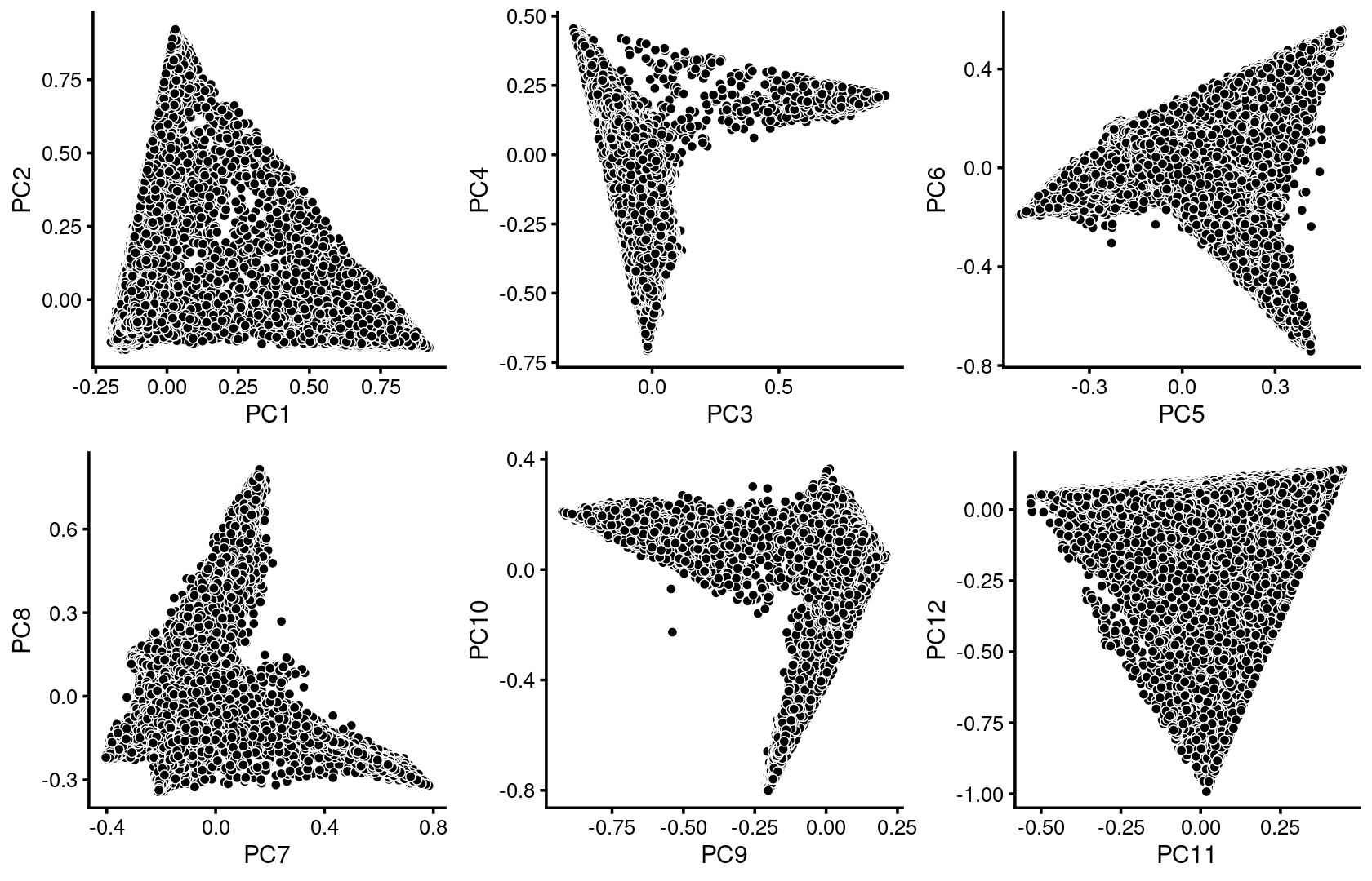
| Version | Author | Date |
|---|---|---|
| a38788b | kevinlkx | 2020-10-20 |
Some of the structure is more evident from “hexbin” plots showing the density of the points.
breaks <- c(0,1,5,10,100,Inf)
p.pca2.1 <- pca_hexbin_plot(poisson2multinom(fit), pcs = 1:2, breaks = breaks) + guides(fill = "none")
p.pca2.2 <- pca_hexbin_plot(poisson2multinom(fit), pcs = 3:4, breaks = breaks) + guides(fill = "none")
p.pca2.3 <- pca_hexbin_plot(poisson2multinom(fit), pcs = 5:6, breaks = breaks) + guides(fill = "none")
p.pca2.4 <- pca_hexbin_plot(poisson2multinom(fit), pcs = 7:8, breaks = breaks) + guides(fill = "none")
p.pca2.5 <- pca_hexbin_plot(poisson2multinom(fit), pcs = 9:10, breaks = breaks) + guides(fill = "none")
p.pca2.6 <- pca_hexbin_plot(poisson2multinom(fit), pcs = 11:12, breaks = breaks) + guides(fill = "none")

plot_grid(p.pca2.1,p.pca2.2,p.pca2.3,p.pca2.4,p.pca2.5,p.pca2.6)
| Version | Author | Date |
|---|---|---|
| a38788b | kevinlkx | 2020-10-20 |
Layer the tissue and cell labels onto the PC plots
Tissues:
samples$tissue <- as.factor(samples$tissue)
cat(length(levels(samples$tissue)), "tissues. \n")
table(samples$tissue)

colors_tissues <- c("darkblue", "darkgray", "red", "springgreen", "brown", "purple", "skyblue", "black",
                    "darkgreen", "plum", "yellow", "orange", "lightgray")
# 13 tissues.
#
#       BoneMarrow       Cerebellum            Heart           Kidney
#             8403             2278             7650             6431
#   LargeIntestine            Liver             Lung PreFrontalCortex
#             7086             6167             9996             5959
#   SmallIntestine           Spleen           Testes           Thymus
#             4077             4020             2723             7617
#       WholeBrain
#             8766
PCs 1 and 2:
p.pca3.1 <- labeled_pca_plot(fit,1:2,samples$tissue,font_size = 7,
                       colors = colors_tissues, legend_label = "tissue")
p.pca3.2 <- labeled_pca_plot(fit,1:2,samples$cell_label,font_size = 7,
                        legend_label = "cell_label")
plot_grid(p.pca3.1,p.pca3.2,rel_widths = c(8,11))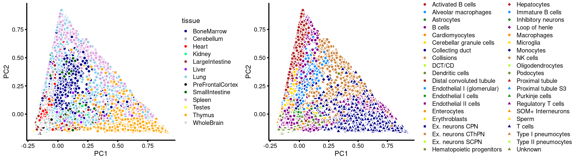
PCs 3 and 4:
p.pca3.3 <- labeled_pca_plot(fit,3:4,samples$tissue,font_size = 7,
                        colors = colors_tissues, legend_label = "tissue")
p.pca3.4 <- labeled_pca_plot(fit,3:4,samples$cell_label,font_size = 7,
                        legend_label = "cell_label")
plot_grid(p.pca3.3,p.pca3.4,rel_widths = c(8,11))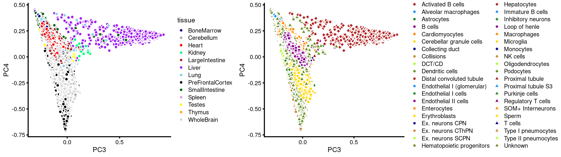
PCs 5 and 6:
p.pca3.5 <- labeled_pca_plot(fit,5:6,samples$tissue,font_size = 7,
                       colors = colors_tissues, legend_label = "tissue")
p.pca3.6 <- labeled_pca_plot(fit,5:6,samples$cell_label,font_size = 7,
                        legend_label = "cell_label")
plot_grid(p.pca3.5,p.pca3.6,rel_widths = c(8,11))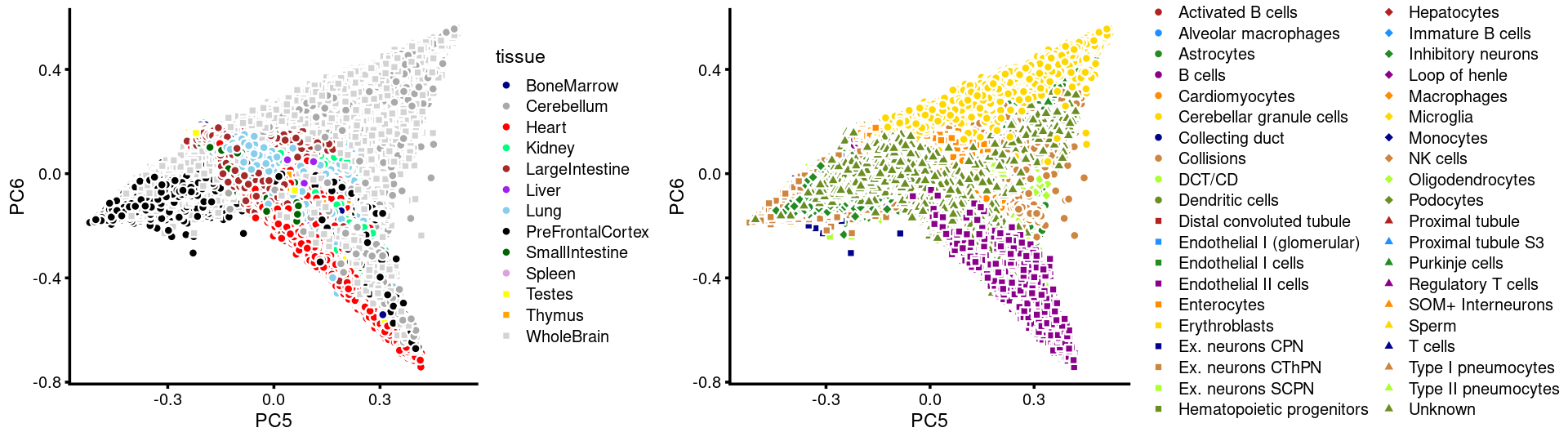
PCs 7 and 8:
p.pca3.7 <- labeled_pca_plot(fit,7:8,samples$tissue,font_size = 7,
                       colors = colors_tissues, legend_label = "tissue")
p.pca3.8 <- labeled_pca_plot(fit,7:8,samples$cell_label,font_size = 7,
                        legend_label = "cell_label")
plot_grid(p.pca3.7,p.pca3.8,rel_widths = c(8,11))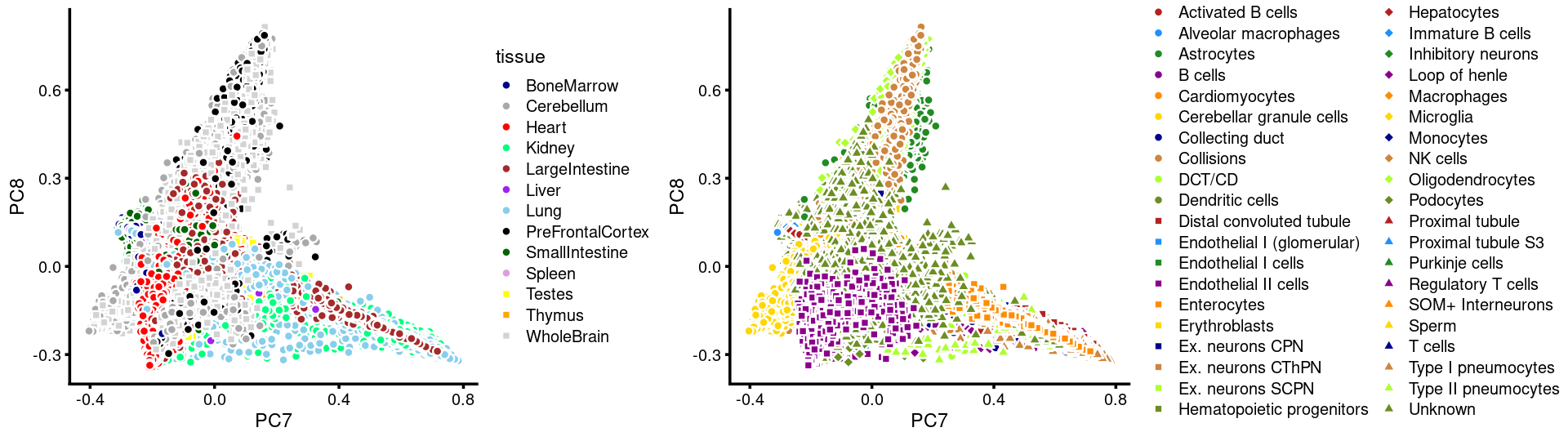
PCs 9 and 10:
p.pca3.9 <- labeled_pca_plot(fit,9:10,samples$tissue,font_size = 7,
                       colors = colors_tissues, legend_label = "tissue")
p.pca3.10 <- labeled_pca_plot(fit,9:10,samples$cell_label,font_size = 7,
                        legend_label = "cell_label")
plot_grid(p.pca3.9,p.pca3.10,rel_widths = c(8,11))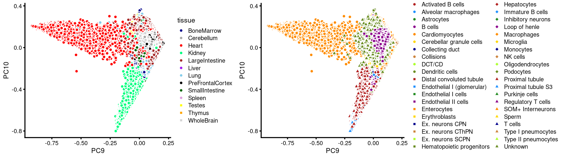
PCs 11 and 12:
p.pca3.11 <- labeled_pca_plot(fit,11:12,samples$tissue,font_size = 7,
                       legend_label = "tissue")
p.pca3.12 <- labeled_pca_plot(fit,11:12,samples$cell_label,font_size = 7,
                        legend_label = "cell_label")
plot_grid(p.pca3.11,p.pca3.12,rel_widths = c(8,11))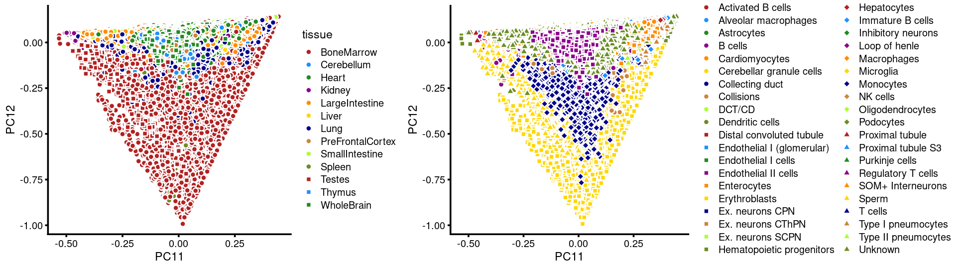
| Version | Author | Date |
|---|---|---|
| a38788b | kevinlkx | 2020-10-20 |
Visualize by structure plot grouped by tissues
set.seed(10)
colors_topics <- c("#a6cee3","#1f78b4","#b2df8a","#33a02c","#fb9a99","#e31a1c",
                   "#fdbf6f","#ff7f00","#cab2d6","#6a3d9a","#ffff99","#b15928",
                   "gray")
rows <- sample(nrow(fit$L),4000)
samples$tissue <- as.factor(samples$tissue)

p.structure.1 <- structure_plot(select(poisson2multinom(fit),loadings = rows),
                     grouping = samples[rows, "tissue"],n = Inf,gap = 40,
                     perplexity = 50,topics = 1:13,colors = colors_topics,
                     num_threads = 4,verbose = FALSE)
# Perplexity automatically changed to 42 because original setting of 50 was too large for the number of samples (132)
# Perplexity automatically changed to 40 because original setting of 50 was too large for the number of samples (124)

print(p.structure.1)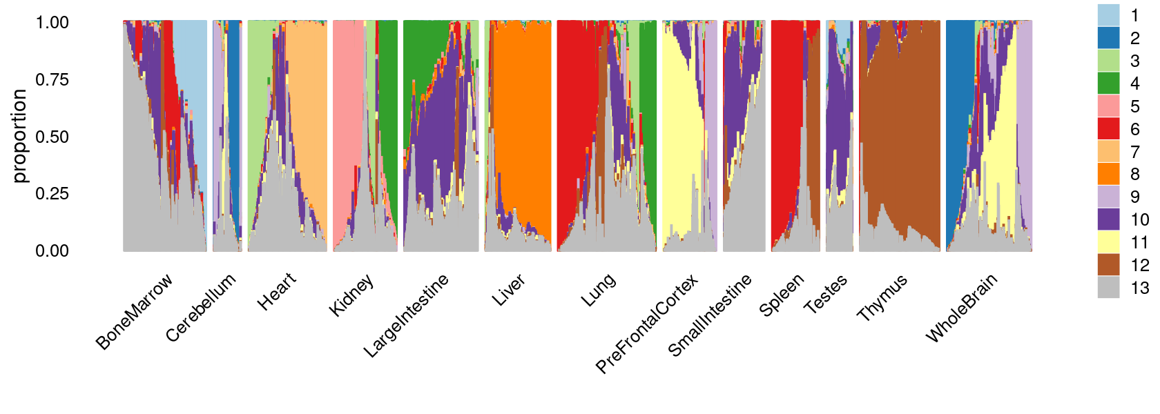
| Version | Author | Date |
|---|---|---|
| 6c97fa9 | kevinlkx | 2020-12-01 |
k-means clustering on topic proportions
Define clusters using k-means, and then create structure plot based on the clusters from k-means.
Define clusters using k-means with 15 clusters:
set.seed(10)

clusters.15 <- factor(kmeans(poisson2multinom(fit)$L,centers = 15)$cluster)
Structure plot based on 15 clusters
colors_topics <- c("#a6cee3","#1f78b4","#b2df8a","#33a02c","#fb9a99","#e31a1c",
            "#fdbf6f","#ff7f00","#cab2d6","#6a3d9a","#ffff99","#b15928",
            "gray")
rows <- sample(nrow(fit$L),4000)

p.structure.kmeans.15 <- structure_plot(select(poisson2multinom(fit),loadings = rows),
                                        grouping = clusters.15[rows],n = Inf,gap = 20,
                                        perplexity = 50,topics = 1:13,colors = colors_topics,
                                        num_threads = 4,verbose = FALSE)
print(p.structure.kmeans.15)
Refine k-means clusters: - Split cluster 10 into two clusters. - (maybe also merge cluster 4 and 9)
set.seed(10)
clusters.refined <- as.numeric(clusters.15)

idx_cluster10 <- which(clusters.15 == 10)
cluster10.refined <- kmeans(poisson2multinom(fit)$L[idx_cluster10, ],centers = 2)$cluster+15
clusters.refined[idx_cluster10] <- cluster10.refined
clusters.refined <- factor(clusters.refined, labels = paste0("c", c(1:length(unique(clusters.refined)))))

samples$cluster_kmeans <- clusters.refined
Save the clustering results to an RDS file
saveRDS(samples, "output/clustering-Cusanovich2018.rds")
samples <- readRDS("output/clustering-Cusanovich2018.rds")
clusters.refined <- samples$cluster_kmeans
print(table(samples$cluster_kmeans))
#
#    c1    c2    c3    c4    c5    c6    c7    c8    c9   c10   c11   c12   c13
#  2740  3868  3775  3879  3645  3651 12037  2955  6045  6068  3582  9319  3411
#   c14   c15   c16
#  4172  6423  5603
Structure plot based on refined clusters
colors_topics <- c("#a6cee3","#1f78b4","#b2df8a","#33a02c","#fb9a99","#e31a1c",
            "#fdbf6f","#ff7f00","#cab2d6","#6a3d9a","#ffff99","#b15928",
            "gray")
rows <- sample(nrow(fit$L),4000)

p.structure.kmeans.refined <- structure_plot(select(poisson2multinom(fit),loadings = rows),
                                             grouping = clusters.refined[rows],n = Inf,gap = 40,
                                             perplexity = 50,topics = 1:13,colors = colors_topics,
                                             num_threads = 4,verbose = FALSE)
print(p.structure.kmeans.refined)
Group samples by k-means clusters first, then by tissue labels:
p.structure.kmeans.refined <- structure_plot(select(poisson2multinom(fit),loadings = rows),
                     grouping = clusters.refined[rows],
                     rows = order(samples[rows, "tissue"]), # samples are grouped by clusters first, then by tissue labels
                     n = Inf,gap = 40,
                     perplexity = 50,topics = 1:13,colors = colors_topics,
                     num_threads = 4,verbose = FALSE)
print(p.structure.kmeans.refined)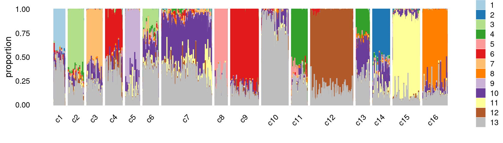
The clusters defined by k-means on topic proportions reasonably identify the clusters shown in the PCA hexbin plots (below).
p.pca.4.1 <- labeled_pca_plot(fit,1:2,samples$cluster_kmeans,font_size = 7,
                       legend_label = "cluster_kmeans")
p.pca.4.2 <- labeled_pca_plot(fit,3:4,samples$cluster_kmeans,font_size = 7,
                       legend_label = "cluster_kmeans")
p.pca.4.3 <- labeled_pca_plot(fit,5:6,samples$cluster_kmeans,font_size = 7,
                       legend_label = "cluster_kmeans")
p.pca.4.4 <- labeled_pca_plot(fit,7:8,samples$cluster_kmeans,font_size = 7,
                       legend_label = "cluster_kmeans")
p.pca.4.5 <- labeled_pca_plot(fit,9:10,samples$cluster_kmeans,font_size = 7,
                       legend_label = "cluster_kmeans")
p.pca.4.6 <- labeled_pca_plot(fit,11:12,samples$cluster_kmeans,font_size = 7,
                       legend_label = "cluster_kmeans")
plot_grid(p.pca.4.1,p.pca.4.2,p.pca.4.3,p.pca.4.4,p.pca.4.5,p.pca.4.6)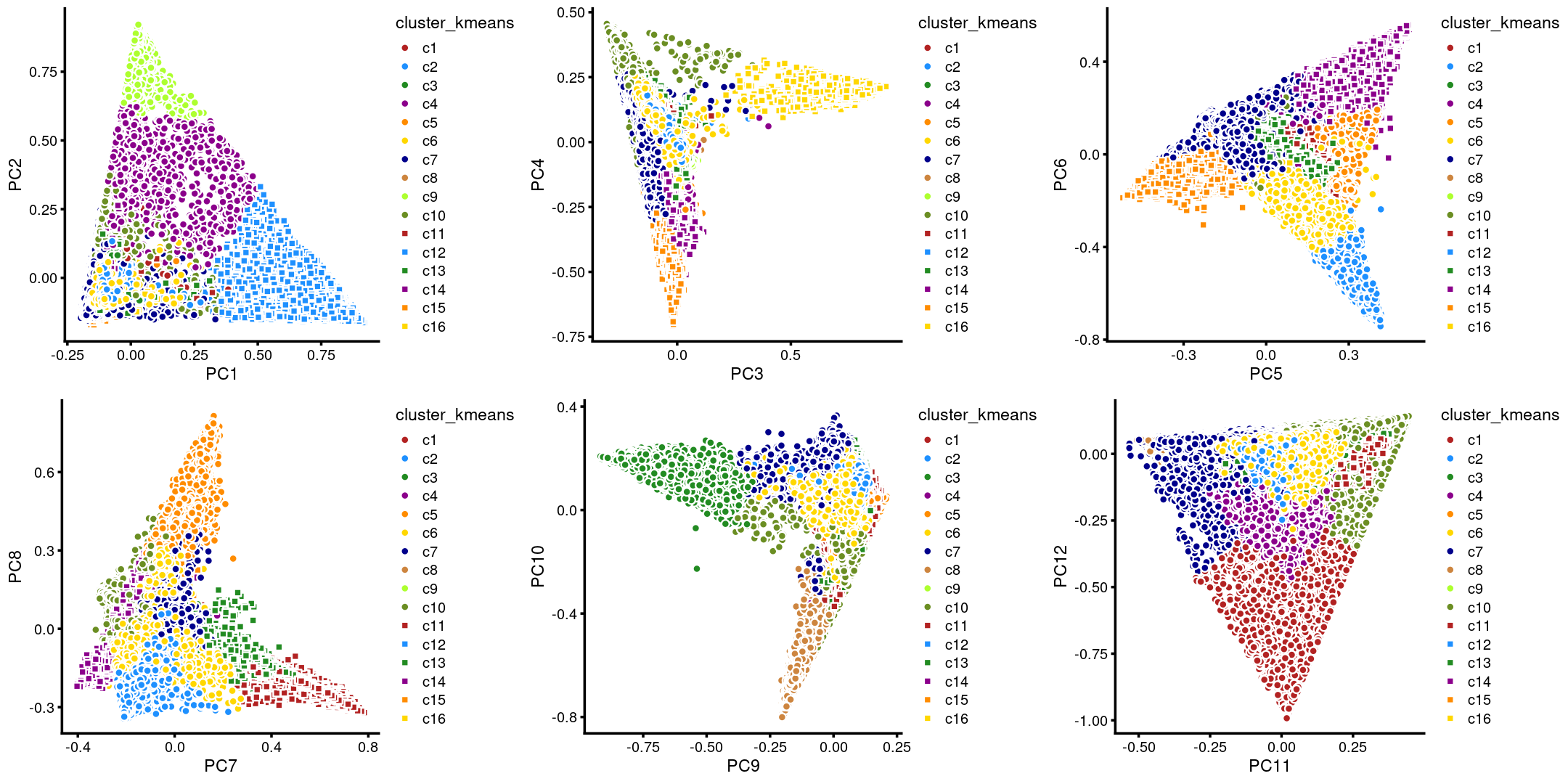
plot_grid(p.pca2.1,p.pca2.2,p.pca2.3,p.pca2.4,p.pca2.5,p.pca2.6)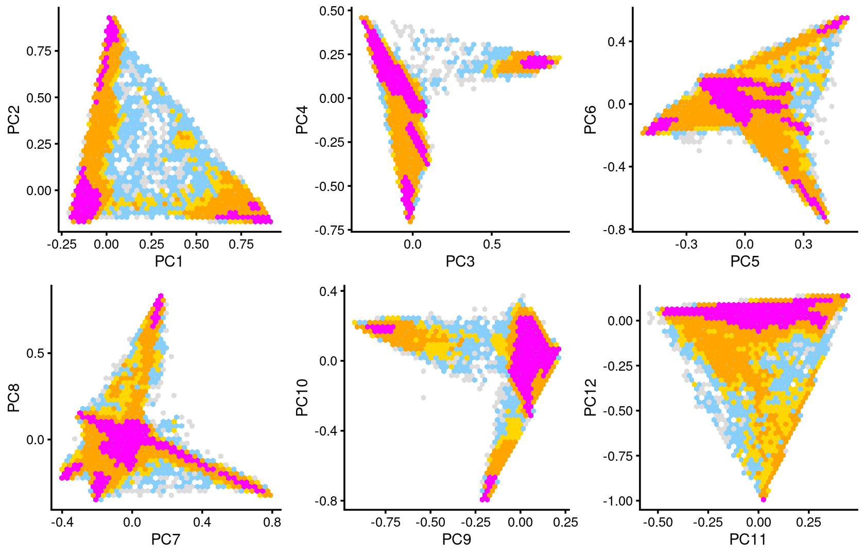
We then label the cells in each cluster with the known tissue labels.
Plot the distribution of tissues by cluster.
Stacked barplot for the counts of tissues by clusters:
library(plyr);library(dplyr)
# ------------------------------------------------------------------------------
# You have loaded plyr after dplyr - this is likely to cause problems.
# If you need functions from both plyr and dplyr, please load plyr first, then dplyr:
# library(plyr); library(dplyr)
# ------------------------------------------------------------------------------
#
# Attaching package: 'plyr'
# The following objects are masked from 'package:dplyr':
#
#     arrange, count, desc, failwith, id, mutate, rename, summarise,
#     summarize
library(RColorBrewer)

freq_cluster_tissue <- count(samples, vars=c("cluster_kmeans","tissue"))

# stacked barplot for the counts of tissues by clusters
p.barplot.1 <- ggplot(freq_cluster_tissue, aes(fill=tissue, y=freq, x=cluster_kmeans)) +
  geom_bar(position="stack", stat="identity") +
  theme_classic() + xlab("Cluster") + ylab("Number of cells") +
  scale_fill_manual(values = colors_tissues) +
  guides(fill=guide_legend(ncol=2)) +
  theme(
  legend.title = element_text(size = 10),
  legend.text = element_text(size = 8)
  )
print(p.barplot.1)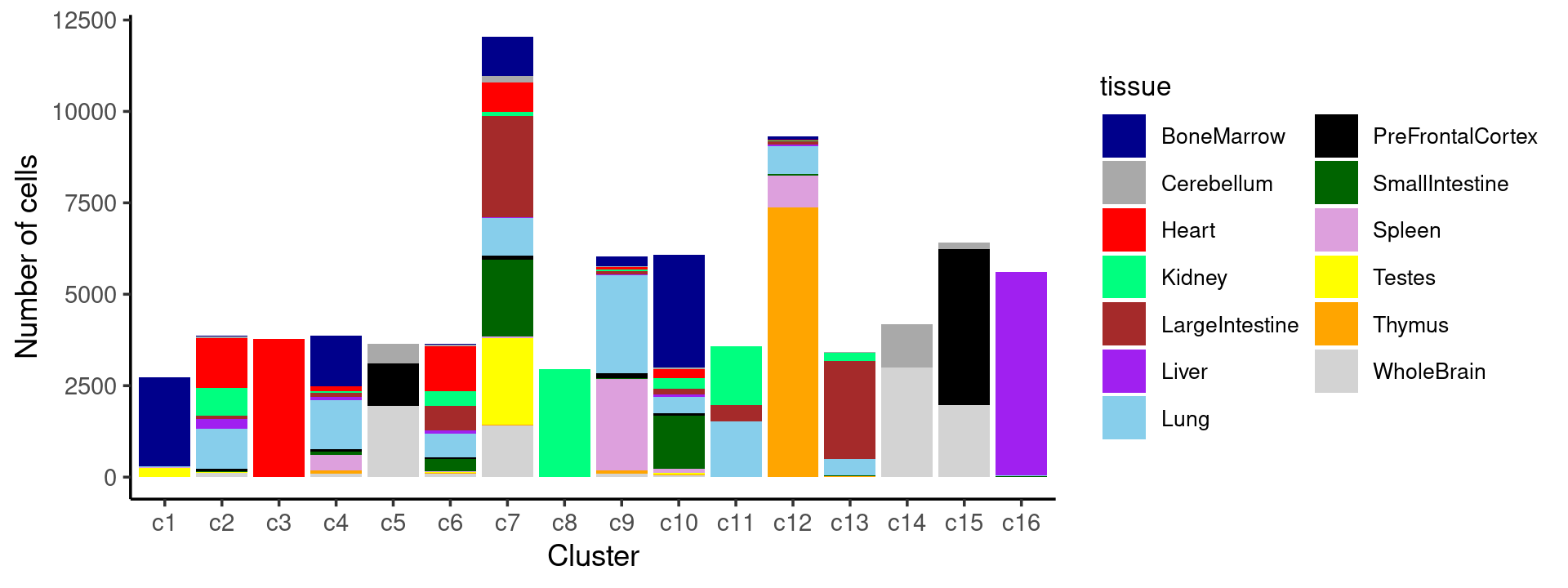
Percent stacked barplot for the counts of tissues by clusters:
p.barplot.2 <- ggplot(freq_cluster_tissue, aes(fill=tissue, y=freq, x=cluster_kmeans)) +
  geom_bar(position="fill", stat="identity") +
  theme_classic() + xlab("Cluster") + ylab("Proportion of cells") +
  scale_fill_manual(values = colors_tissues) +
  guides(fill=guide_legend(ncol=2)) +
  theme(
  legend.title = element_text(size = 10),
  legend.text = element_text(size = 8)
  )
print(p.barplot.2)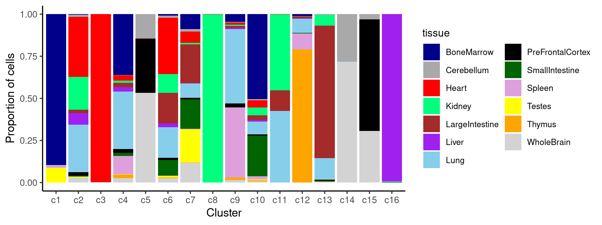
We can see a few clusters are tissue specific:
- cluster c3 is heart specific;
- cluster c8 is kidney specific;
- cluster c16 is liver specific;
- cluster c1 is primarily bone marrow;
- cluster c12 is primarily thymus.
Some clusters are combinations of related tissues:
- cluster c9 is half lung and half spleen;
- cluster c5 and c15 are mainly from pre-frontal cortex, whole brain (and cerebellum) -- all neuron related.
- cluster c14 is also from whole brain and cerebellum.
- cluster c11 is mainly from Kidney, LargeIntestine, and Lung.
Some clusters are more heterogeneous mixtures of different tissues: e.g. c2, c6, c7, c12.
freq_table_cluster_tissue <- with(samples,table(tissue,cluster_kmeans))
print(freq_table_cluster_tissue)
#                   cluster_kmeans
# tissue               c1   c2   c3   c4   c5   c6   c7   c8   c9  c10  c11  c12
#   BoneMarrow       2455   15    0 1399    0   33 1060    0  276 3063    0  102
#   Cerebellum          0   51    0    7  525   44  191    0   30   42    0    0
#   Heart               0 1374 3768  126    3 1225  803    5   68  259    3   13
#   Kidney              0  757    0   47    0  402   98 2950   48  280 1614   19
#   LargeIntestine      0   73    1  107    4  665 2778    0   71  172  441   94
#   Liver               0  268    0   97    0   84   31    0   39   50    1   34
#   Lung                2 1093    5 1324    2  659 1010    0 2678  465 1521  773
#   PreFrontalCortex    0   75    0   84 1169   48  118    0  131   49    0    1
#   SmallIntestine      0   22    0   75    0  341 2112    0    9 1457    1   27
#   Spleen             43    3    0  427    0    5   24    0 2510  116    0  892
#   Testes            240   19    0    1    0   37 2379    0    2   38    0    0
#   Thymus              0    2    1   82    0    9   32    0   90   30    1 7363
#   WholeBrain          0  116    0  103 1942   99 1401    0   93   47    0    1
#                   cluster_kmeans
# tissue              c13  c14  c15  c16
#   BoneMarrow          0    0    0    0
#   Cerebellum         15 1177  196    0
#   Heart               3    0    0    0
#   Kidney            215    0    0    1
#   LargeIntestine   2680    0    0    0
#   Liver               4    1    0 5558
#   Lung              434    2    2   26
#   PreFrontalCortex   19    4 4261    0
#   SmallIntestine     18    0    0   15
#   Spleen              0    0    0    0
#   Testes              4    0    0    3
#   Thymus              7    0    0    0
#   WholeBrain         12 2988 1964    0
Plot the distribution of cell labels by cluster.
Cell labels:
samples$cell_label <- as.factor(samples$cell_label)
cat(length(levels(samples$cell_label)), "cell labels. \n")
table(samples$cell_label)

colors_celllabels <- c(colorRampPalette(brewer.pal(12, "Set3"))(39), "black")
names(colors_celllabels) <- levels(samples$cell_label)
colors_celllabels[grep("Cardio", names(colors_celllabels))] <- "red"
colors_celllabels[grep("Endothelial", names(colors_celllabels))] <- "plum"
colors_celllabels[grep("neuron", names(colors_celllabels))] <- "gray"
colors_celllabels[grep("pneumocytes", names(colors_celllabels))] <- "skyblue"
colors_celllabels[grep("tubule", names(colors_celllabels))] <- "purple"
# 40 cell labels.
#
#          Activated B cells       Alveolar macrophages
#                        500                        559
#                 Astrocytes                    B cells
#                       1666                       5772
#             Cardiomyocytes   Cerebellar granule cells
#                       4076                       4099
#            Collecting duct                 Collisions
#                        164                       1218
#                     DCT/CD            Dendritic cells
#                        506                        958
#   Distal convoluted tubule Endothelial I (glomerular)
#                        319                        552
#        Endothelial I cells       Endothelial II cells
#                        952                       3019
#                Enterocytes              Erythroblasts
#                       4783                       2811
#            Ex. neurons CPN          Ex. neurons CThPN
#                       1832                       1540
#           Ex. neurons SCPN  Hematopoietic progenitors
#                       1466                       3425
#                Hepatocytes           Immature B cells
#                       5664                        571
#         Inhibitory neurons              Loop of henle
#                       1828                        815
#                Macrophages                  Microglia
#                        711                        422
#                  Monocytes                   NK cells
#                       1173                        321
#           Oligodendrocytes                  Podocytes
#                       1558                        498
#            Proximal tubule         Proximal tubule S3
#                       2570                        594
#             Purkinje cells         Regulatory T cells
#                        320                        507
#          SOM+ Interneurons                      Sperm
#                        553                       2089
#                    T cells         Type I pneumocytes
#                       8954                       1622
#        Type II pneumocytes                    Unknown
#                        157                      10029
Stacked barplot for the counts of cell labels by clusters:
freq_cluster_celllabel <- count(samples, vars=c("cluster_kmeans","cell_label"))

# stacked barplot for the counts of tissues by clusters
p.barplot.3 <- ggplot(freq_cluster_celllabel, aes(fill=cell_label, y=freq, x=cluster_kmeans)) +
  geom_bar(position="stack", stat="identity") +
  theme_classic() + xlab("Cluster") + ylab("Number of cells") +
  scale_fill_manual(values = colors_celllabels) +
  guides(fill=guide_legend(ncol=3)) +
  theme(
  legend.title = element_text(size = 9),
  legend.text = element_text(size = 7)
  )
print(p.barplot.3)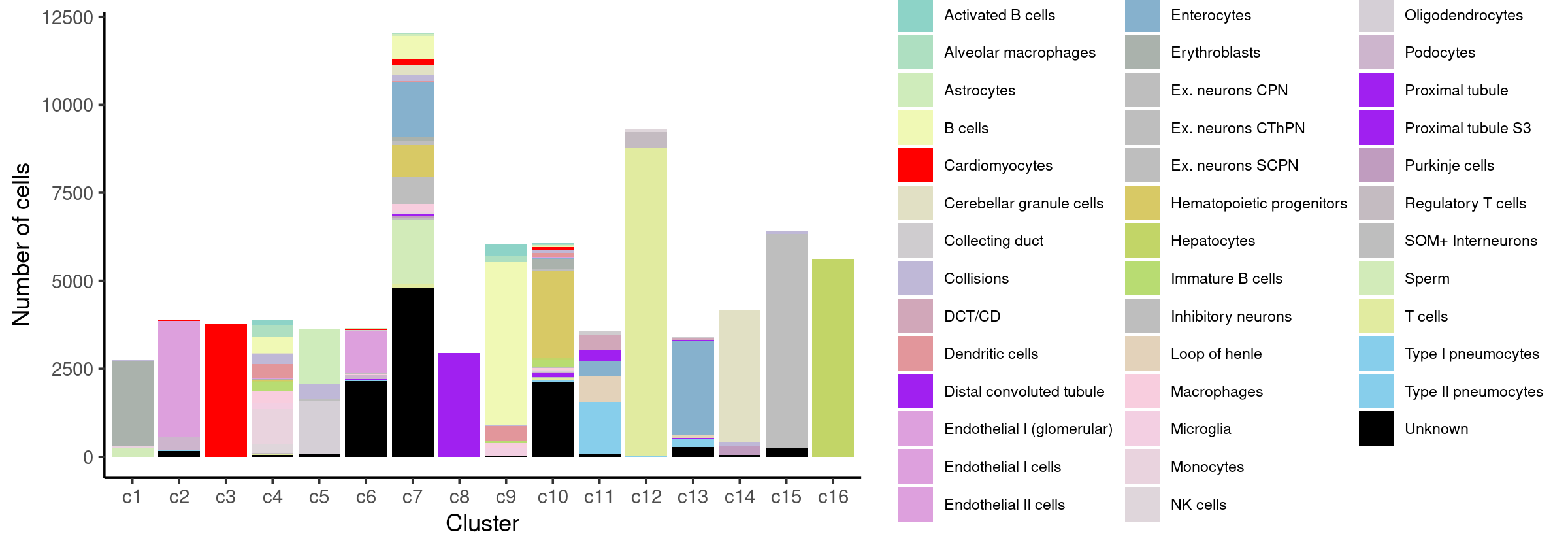
Percent stacked barplot for the counts of tissues by clusters:
p.barplot.4 <- ggplot(freq_cluster_celllabel, aes(fill=cell_label, y=freq, x=cluster_kmeans)) +
  geom_bar(position="fill", stat="identity") +
  theme_classic() + xlab("Cluster") + ylab("Proportion of cells") +
  scale_fill_manual(values = colors_celllabels) +
  guides(fill=guide_legend(ncol=3)) +
  theme(
  legend.title = element_text(size = 9),
  legend.text = element_text(size = 7)
  )
print(p.barplot.4)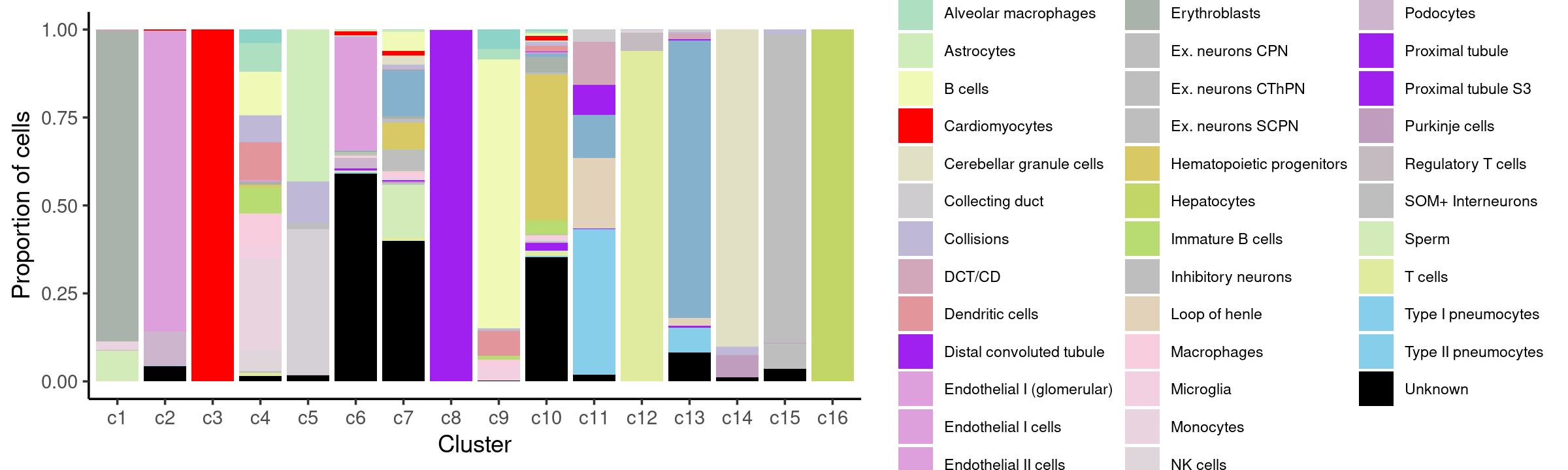
freq_table_cluster_celllabel <- with(samples,table(cell_label,cluster_kmeans))
print(freq_table_cluster_celllabel)
#                             cluster_kmeans
# cell_label                     c1   c2   c3   c4   c5   c6   c7   c8   c9  c10
#   Activated B cells             0    0    0  146    0    0    0    0  331   23
#   Alveolar macrophages          0    0    0  322    0    2   16    0  185   34
#   Astrocytes                    0    0    0    0 1574   11   58    0    0   20
#   B cells                       0    0    0  470    0    3  648    0 4616   34
#   Cardiomyocytes                0   15 3773    1    0   42  169    0    0   76
#   Cerebellar granule cells      0    0    0    9    0    3  306    0    0   19
#   Collecting duct               0    0    0    0    0   10    0    0    0    5
#   Collisions                    6    2    0  296  423   15  166    0   44   64
#   DCT/CD                        0    0    0    0    0    1    0    1    0    6
#   Dendritic cells               1    0    0  416    0    2   12    0  424  102
#   Distal convoluted tubule      0    0    0    0    0    0    0    0    0    6
#   Endothelial I (glomerular)    0  386    0    0    0  158    0    0    0    8
#   Endothelial I cells           0  512    0    0    0  438    1    0    0    1
#   Endothelial II cells          0 2405    0   15    0  574    7    0    0   15
#   Enterocytes                   0    0    0    0    1   11 1585    0    0   54
#   Erythroblasts              2420    0    0   37    0    0   79    0    0  275
#   Ex. neurons CPN               0    0    0    0    0    0   10    0    0    0
#   Ex. neurons CThPN             0    0    0    0    0    0   91    0    0    0
#   Ex. neurons SCPN              0    0    0    0    0    0   40    0    0   32
#   Hematopoietic progenitors     0    0    0   26    0    1  899    0    0 2499
#   Hepatocytes                   0    0    0    2    0    5   11    0    0   44
#   Immature B cells              0    0    0  285    0    0    0    0   68  218
#   Inhibitory neurons            0    0    0    3   68   27  754    0    0    8
#   Loop of henle                 0    1    0    0    0    8    2    1    0   11
#   Macrophages                   0    0    0  337    0   14  191    0  127   42
#   Microglia                     0    1    0  159    1    3   31    0  226    1
#   Monocytes                    69    0    0 1010    0    1   50    0    9   32
#   NK cells                      0    0    0  231    0    1    2    0    0   16
#   Oligodendrocytes              0    0    0    1 1506    1   30    0    0   17
#   Podocytes                     0  369    0    0    0  113    0    0    0   16
#   Proximal tubule               0    1    0    1    0   16   33 2361    0  132
#   Proximal tubule S3            0    0    0    0    0    0    2  592    0    0
#   Purkinje cells                0    0    0    0    1    2   50    0    0    0
#   Regulatory T cells            3    0    0   17    0    1    7    0    0    4
#   SOM+ Interneurons             0    0    0    0    7    8   66    0    0    5
#   Sperm                       240    0    0    0    0    1 1814    0    0   32
#   T cells                       1    1    0   35    1    7  104    0    0   50
#   Type I pneumocytes            0    0    0    1    0    3    0    0    0   27
#   Type II pneumocytes           0    8    0    0    0   14    0    0    0    1
#   Unknown                       0  167    2   59   63 2155 4803    0   15 2139
#                             cluster_kmeans
# cell_label                    c11  c12  c13  c14  c15  c16
#   Activated B cells             0    0    0    0    0    0
#   Alveolar macrophages          0    0    0    0    0    0
#   Astrocytes                    0    0    0    0    3    0
#   B cells                       0    0    1    0    0    0
#   Cardiomyocytes                0    0    0    0    0    0
#   Cerebellar granule cells      0    0    0 3762    0    0
#   Collecting duct             124    0   25    0    0    0
#   Collisions                    0   11    8   97   86    0
#   DCT/CD                      441    0   57    0    0    0
#   Dendritic cells               0    0    1    0    0    0
#   Distal convoluted tubule    301    0   12    0    0    0
#   Endothelial I (glomerular)    0    0    0    0    0    0
#   Endothelial I cells           0    0    0    0    0    0
#   Endothelial II cells          0    1    1    1    0    0
#   Enterocytes                 442    0 2690    0    0    0
#   Erythroblasts                 0    0    0    0    0    0
#   Ex. neurons CPN               0    0    0    0 1822    0
#   Ex. neurons CThPN             0    0    0    0 1449    0
#   Ex. neurons SCPN              0    0    0    0 1394    0
#   Hematopoietic progenitors     0    0    0    0    0    0
#   Hepatocytes                   0    0    0    0    0 5602
#   Immature B cells              0    0    0    0    0    0
#   Inhibitory neurons            0    0    0    3  965    0
#   Loop of henle               718    0   74    0    0    0
#   Macrophages                   0    0    0    0    0    0
#   Microglia                     0    0    0    0    0    0
#   Monocytes                     0    2    0    0    0    0
#   NK cells                      0   71    0    0    0    0
#   Oligodendrocytes              0    0    0    0    3    0
#   Podocytes                     0    0    0    0    0    0
#   Proximal tubule               7    0   19    0    0    0
#   Proximal tubule S3            0    0    0    0    0    0
#   Purkinje cells                0    0    0  262    5    0
#   Regulatory T cells            0  475    0    0    0    0
#   SOM+ Interneurons             0    0    0    1  466    0
#   Sperm                         0    0    2    0    0    0
#   T cells                       0 8753    2    0    0    0
#   Type I pneumocytes         1415    6  170    0    0    0
#   Type II pneumocytes          66    0   68    0    0    0
#   Unknown                      68    0  281   46  230    1
zoom into a few clusters:
zoom into cluster c2
rows.c2 <- which(samples$cluster_kmeans == "c2")Structure plot of c2 cluster: Group samples by tissue labels first, then by cell labels
tissue_labels_c2 <- as.factor(as.character(samples[rows.c2, "tissue"]))
cell_labels_c2 <- as.factor(as.character(samples[rows.c2, "cell_label"]))

p.structure.c2.1 <- structure_plot(select(poisson2multinom(fit),loadings = rows.c2),
                     grouping = tissue_labels_c2,
                     rows = order(cell_labels_c2),
                     n = Inf,gap = 40,
                     perplexity = 50,topics = 1:13,colors = colors_topics,
                     num_threads = 4,verbose = FALSE)
print(p.structure.c2.1)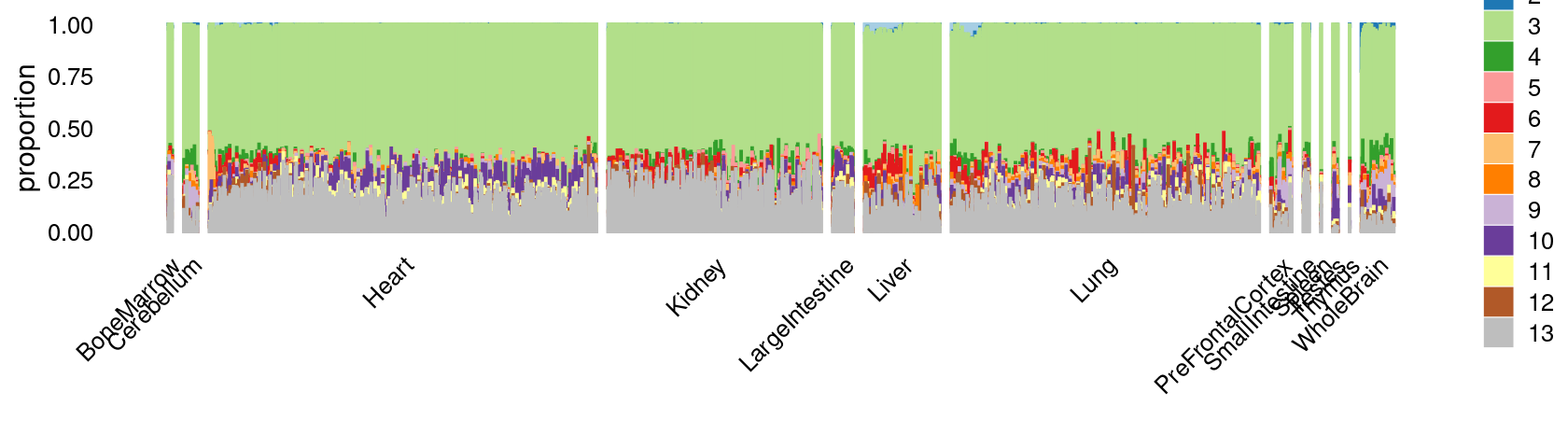
| Version | Author | Date |
|---|---|---|
| 96392bf | kevinlkx | 2020-12-02 |
breaks <- c(0,1,5,10,100,Inf)

fit.c2 <- select(poisson2multinom(fit),loadings = rows.c2)
p.pca.c2 <- pca_plot(fit.c2,fill = "none")
p.pca.hexbin.c2 <- pca_hexbin_plot(fit.c2,breaks = breaks) + guides(fill = "none")
plot_grid(p.pca.c2, p.pca.hexbin.c2)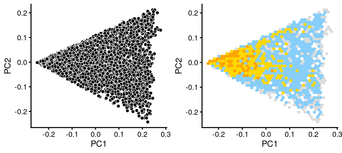
| Version | Author | Date |
|---|---|---|
| 96392bf | kevinlkx | 2020-12-02 |
The variation in PCs 1 and 2 is mostly produced by topics 3,4,9,10,13
p.pca.c2.topics <- pca_plot(fit.c2,k = c(3,4,9,10,13))
print(p.pca.c2.topics)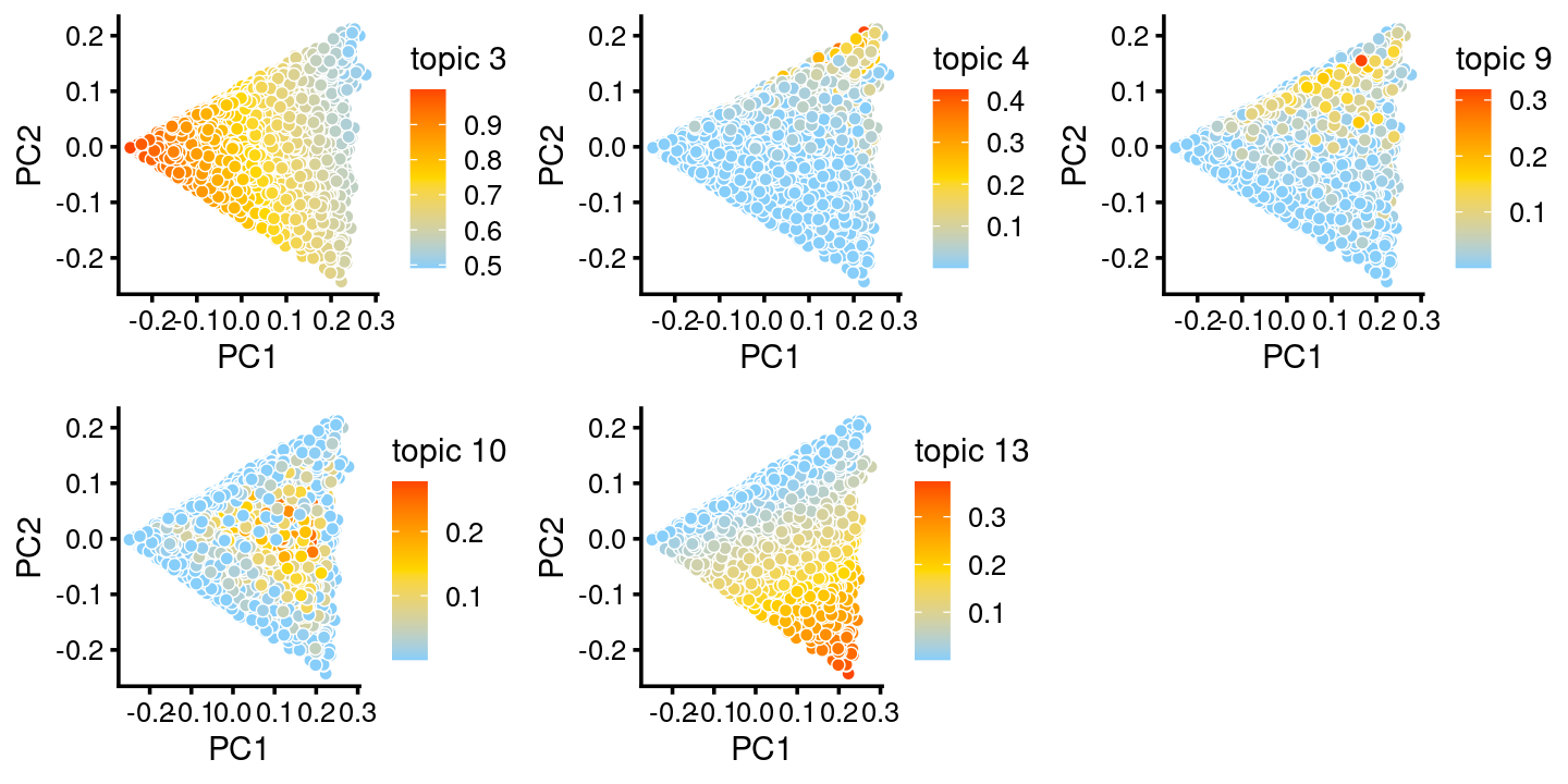
print(table(as.character(samples[rows.c2, "tissue"])))

print(table(as.character(samples[rows.c2, "cell_label"])))

colors_celllabels_c2 <- c("firebrick","dodgerblue","forestgreen",
                           "darkmagenta","darkorange","gold","darkblue",
                           "peru","greenyellow","olivedrab",
                           "darkgray", "black")

p.pca.c2.tissue <- labeled_pca_plot(fit.c2,1:2,samples[rows.c2, "tissue"],font_size = 7,
                       colors = colors_tissues, legend_label = "tissue")
p.pca.c2.cell <- labeled_pca_plot(fit.c2,1:2,samples[rows.c2, "cell_label"],font_size = 7,
                        colors = colors_celllabels_c2, legend_label = "cell_label")
plot_grid(p.pca.c2.tissue,p.pca.c2.cell,rel_widths = c(8,9))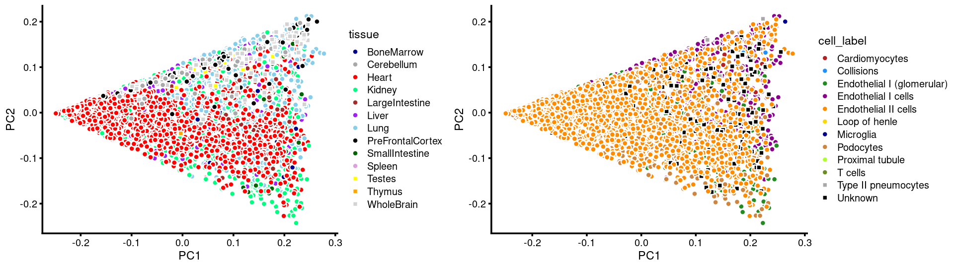
| Version | Author | Date |
|---|---|---|
| 96392bf | kevinlkx | 2020-12-02 |
#
#       BoneMarrow       Cerebellum            Heart           Kidney
#               15               51             1374              757
#   LargeIntestine            Liver             Lung PreFrontalCortex
#               73              268             1093               75
#   SmallIntestine           Spleen           Testes           Thymus
#               22                3               19                2
#       WholeBrain
#              116
#
#             Cardiomyocytes                 Collisions
#                         15                          2
# Endothelial I (glomerular)        Endothelial I cells
#                        386                        512
#       Endothelial II cells              Loop of henle
#                       2405                          1
#                  Microglia                  Podocytes
#                          1                        369
#            Proximal tubule                    T cells
#                          1                          1
#        Type II pneumocytes                    Unknown
#                          8                        167
zoom into cluster c5
rows.c5 <- which(samples$cluster_kmeans == "c5")Structure plot of c5 cluster: Group samples by tissue labels first, then by cell labels
tissue_labels_c5 <- as.factor(as.character(samples[rows.c5, "tissue"]))
cell_labels_c5 <- as.factor(as.character(samples[rows.c5, "cell_label"]))

p.structure.c5.1 <- structure_plot(select(poisson2multinom(fit),loadings = rows.c5),
                     grouping = tissue_labels_c5,
                     rows = order(cell_labels_c5),
                     n = Inf,gap = 40,
                     perplexity = 50,topics = 1:13,colors = colors_topics,
                     num_threads = 4,verbose = FALSE)
print(p.structure.c5.1)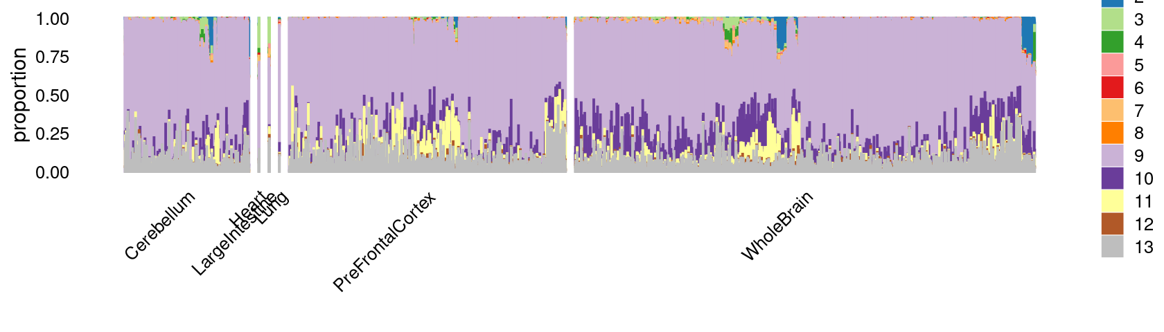
| Version | Author | Date |
|---|---|---|
| 96392bf | kevinlkx | 2020-12-02 |
breaks <- c(0,1,5,10,100,Inf)

fit.c5 <- select(poisson2multinom(fit),loadings = rows.c5)
p.pca.c5 <- pca_plot(fit.c5,fill = "none")
p.pca.hexbin.c5 <- pca_hexbin_plot(fit.c5,breaks = breaks) + guides(fill = "none")
plot_grid(p.pca.c5, p.pca.hexbin.c5)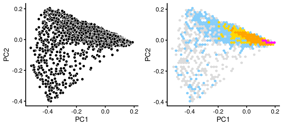
| Version | Author | Date |
|---|---|---|
| 96392bf | kevinlkx | 2020-12-02 |
The variation in PCs 1 and 2 is mostly produced by topics 2,9,10,11,13
p.pca.c5.topics <- pca_plot(fit.c5,k = c(2,9,10,11,13))
print(p.pca.c5.topics)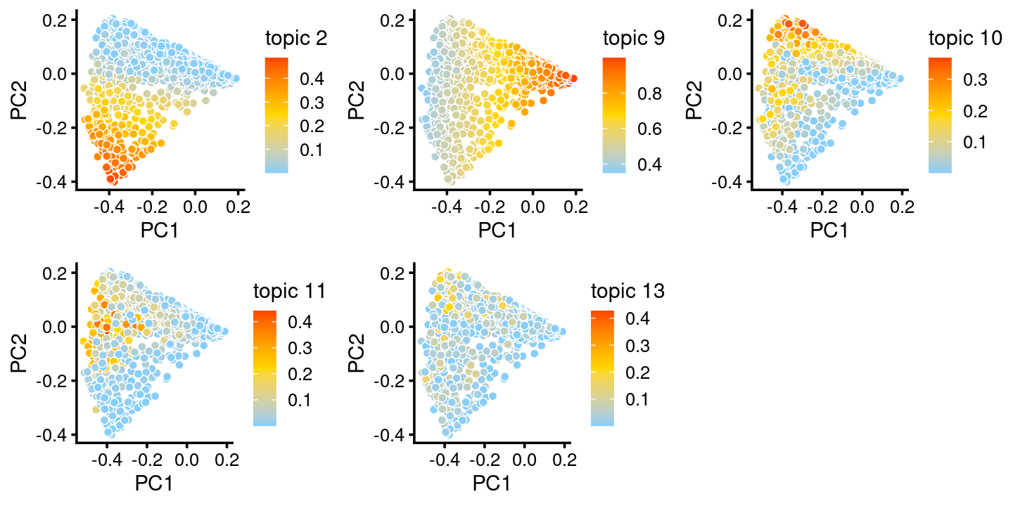
print(table(as.character(samples[rows.c5, "tissue"])))

print(table(as.character(samples[rows.c5, "cell_label"])))

colors_celllabels_c5 <- c("firebrick","dodgerblue","forestgreen",
                           "darkmagenta","darkorange","gold","darkblue",
                           "peru","greenyellow","black")

p.pca.c5.tissue <- labeled_pca_plot(fit.c5,1:2,samples[rows.c5, "tissue"],font_size = 7,
                       colors = colors_tissues, legend_label = "tissue")
p.pca.c5.cell <- labeled_pca_plot(fit.c5,1:2,samples[rows.c5, "cell_label"],font_size = 7,
                        colors = colors_celllabels_c5, legend_label = "cell_label")
plot_grid(p.pca.c5.tissue,p.pca.c5.cell,rel_widths = c(8,11))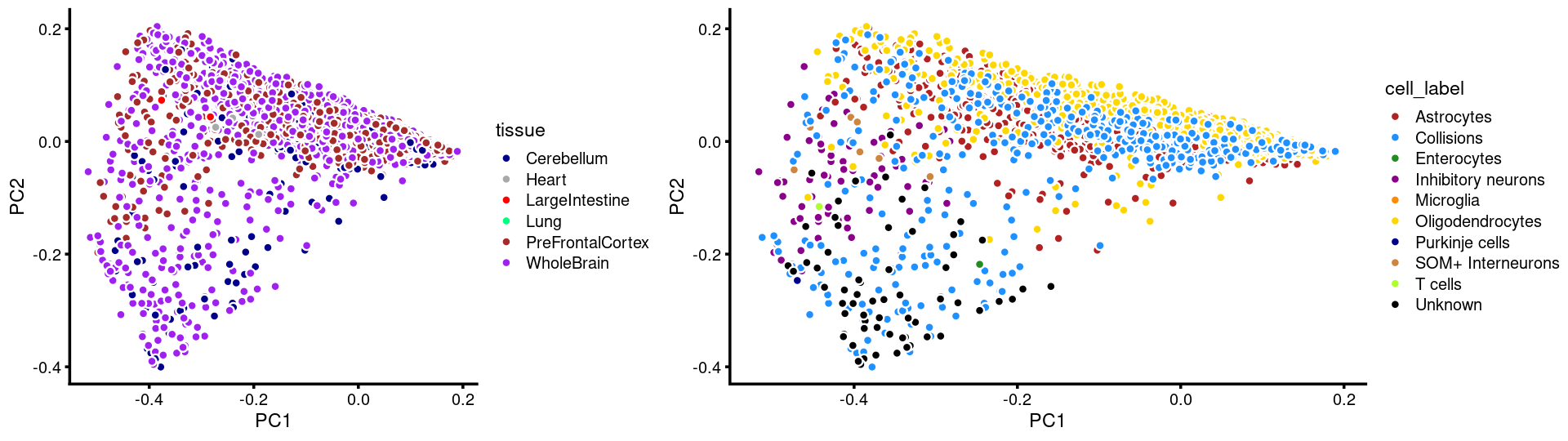
| Version | Author | Date |
|---|---|---|
| 96392bf | kevinlkx | 2020-12-02 |
#
#       Cerebellum            Heart   LargeIntestine             Lung
#              525                3                4                2
# PreFrontalCortex       WholeBrain
#             1169             1942
#
#         Astrocytes         Collisions        Enterocytes Inhibitory neurons
#               1574                423                  1                 68
#          Microglia   Oligodendrocytes     Purkinje cells  SOM+ Interneurons
#                  1               1506                  1                  7
#            T cells            Unknown
#                  1                 63
zoom into cluster c15
rows.c15 <- which(samples$cluster_kmeans == "c15")Structure plot of c15 cluster: Group samples by tissue labels first, then by cell labels
tissue_labels_c15 <- as.factor(as.character(samples[rows.c15, "tissue"]))
cell_labels_c15 <- as.factor(as.character(samples[rows.c15, "cell_label"]))

p.structure.c15.1 <- structure_plot(select(poisson2multinom(fit),loadings = rows.c15),
                     grouping = tissue_labels_c15,
                     rows = order(cell_labels_c15),
                     n = Inf,gap = 40,
                     perplexity = 50,topics = 1:13,colors = colors_topics,
                     num_threads = 4,verbose = FALSE)
print(p.structure.c15.1)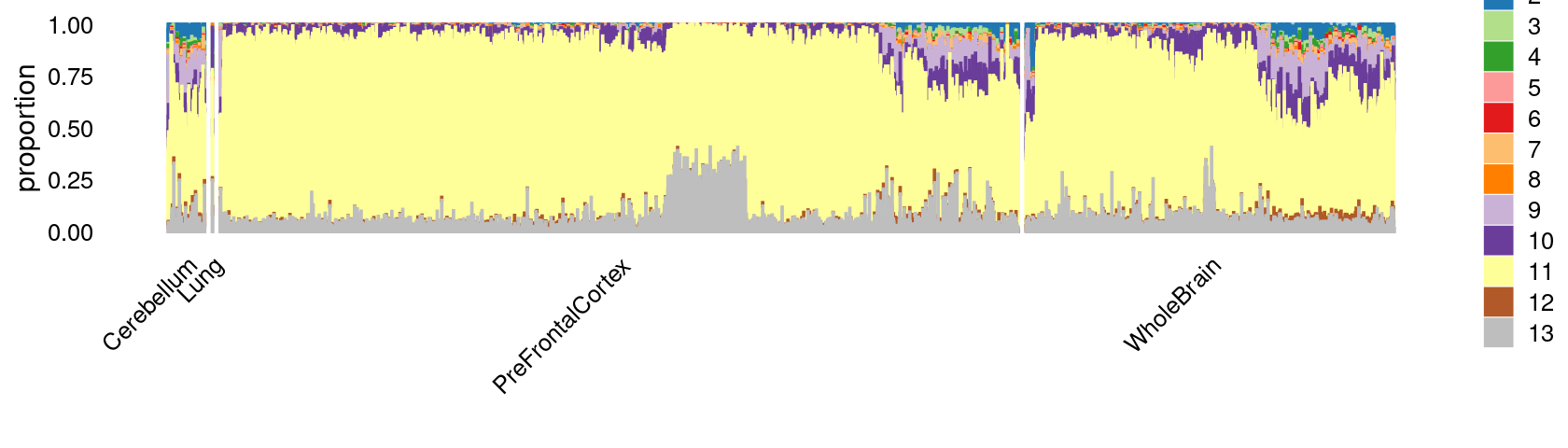
| Version | Author | Date |
|---|---|---|
| 96392bf | kevinlkx | 2020-12-02 |
breaks <- c(0,1,5,10,100,Inf)

fit.c15 <- select(poisson2multinom(fit),loadings = rows.c15)
p.pca.c15 <- pca_plot(fit.c15,fill = "none")
p.pca.hexbin.c15 <- pca_hexbin_plot(fit.c15,breaks = breaks) + guides(fill = "none")
plot_grid(p.pca.c15, p.pca.hexbin.c15)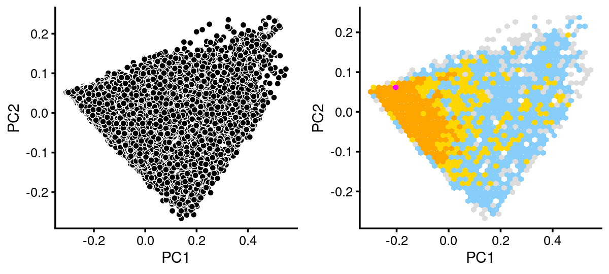
| Version | Author | Date |
|---|---|---|
| 96392bf | kevinlkx | 2020-12-02 |
The variation in PCs 1 and 2 is mostly produced by topics 9,10,11
p.pca.c15.topics <- pca_plot(fit.c15,k = c(9,10,11))
print(p.pca.c15.topics)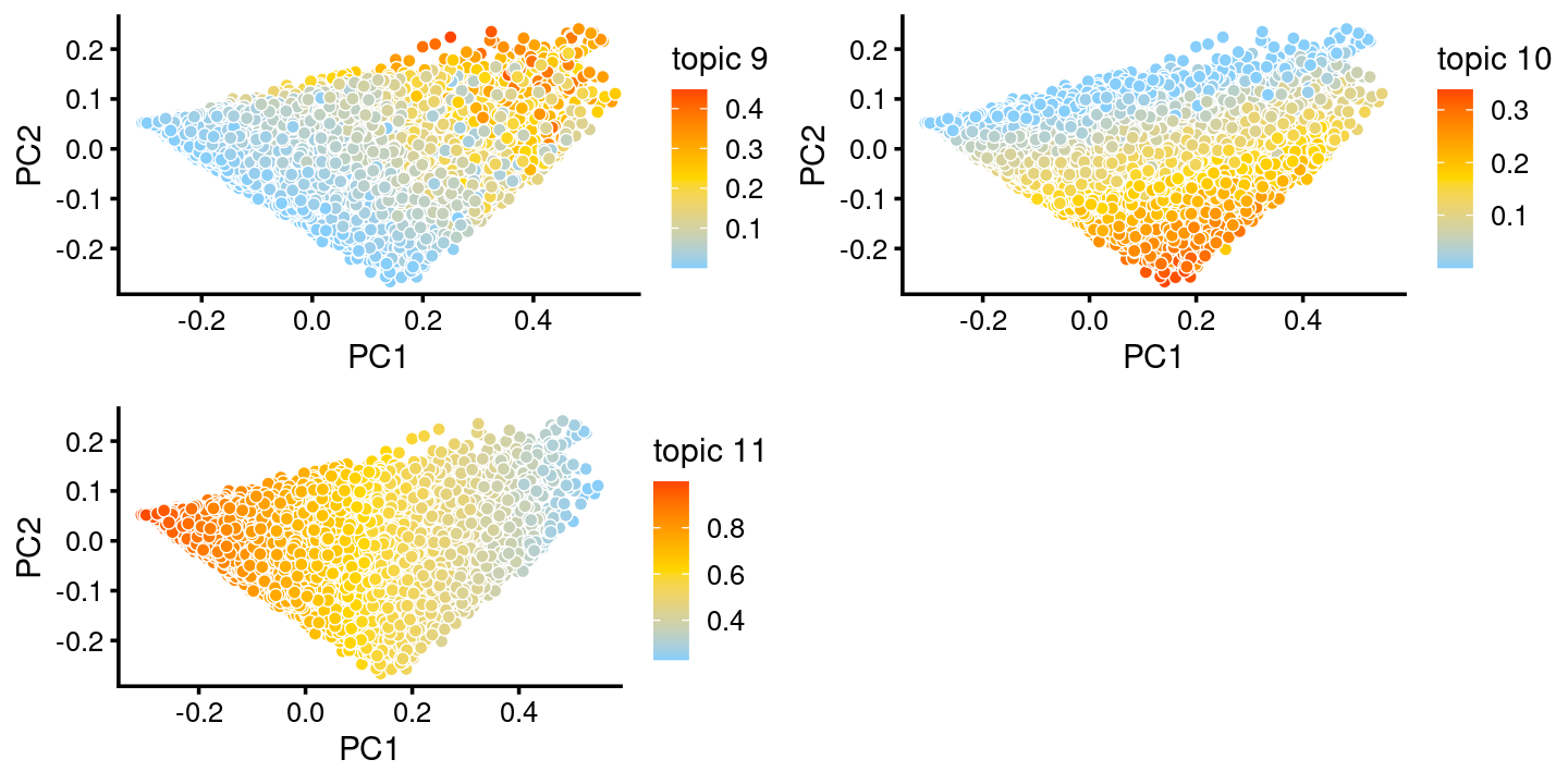
print(table(as.character(samples[rows.c15, "tissue"])))

print(table(as.character(samples[rows.c15, "cell_label"])))

colors_celllabels_c15 <- c("firebrick","dodgerblue","forestgreen",
                           "darkmagenta","darkorange","gold","darkblue",
                           "peru","greenyellow","black")

p.pca.c15.tissue <- labeled_pca_plot(fit.c15,1:2,samples[rows.c15, "tissue"],font_size = 7,
                       colors = colors_tissues, legend_label = "tissue")
p.pca.c15.cell <- labeled_pca_plot(fit.c15,1:2,samples[rows.c15, "cell_label"],font_size = 7,
                        colors = colors_celllabels_c15, legend_label = "cell_label")
plot_grid(p.pca.c15.tissue,p.pca.c15.cell,rel_widths = c(8,11))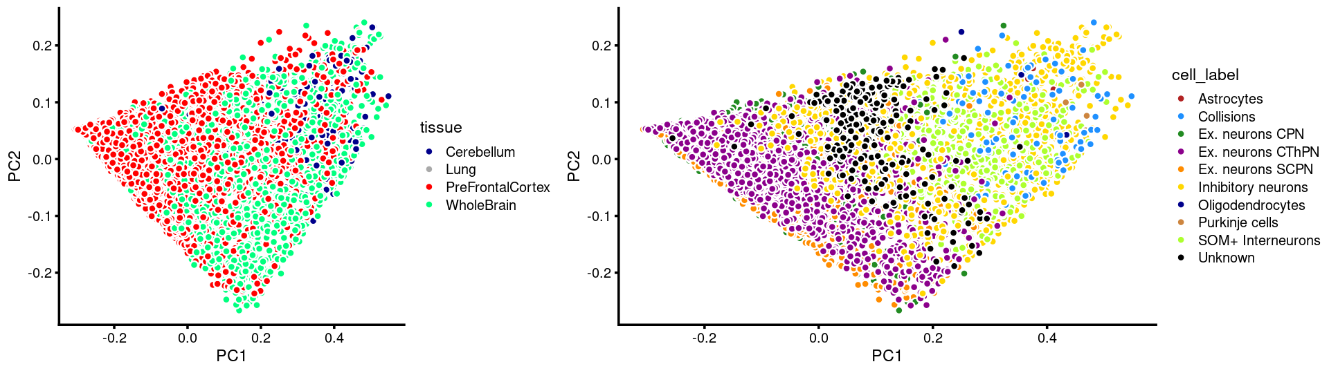
| Version | Author | Date |
|---|---|---|
| 96392bf | kevinlkx | 2020-12-02 |
#
#       Cerebellum             Lung PreFrontalCortex       WholeBrain
#              196                2             4261             1964
#
#         Astrocytes         Collisions    Ex. neurons CPN  Ex. neurons CThPN
#                  3                 86               1822               1449
#   Ex. neurons SCPN Inhibitory neurons   Oligodendrocytes     Purkinje cells
#               1394                965                  3                  5
#  SOM+ Interneurons            Unknown
#                466                230
zoom into cluster c6
rows.c6 <- which(samples$cluster_kmeans == "c6")Structure plot of c6 cluster: Group samples by tissue labels first, then by cell labels
tissue_labels_c6 <- as.factor(as.character(samples[rows.c6, "tissue"]))
cell_labels_c6 <- as.factor(as.character(samples[rows.c6, "cell_label"]))

p.structure.c6.1 <- structure_plot(select(poisson2multinom(fit),loadings = rows.c6),
                     grouping = tissue_labels_c6,
                     rows = order(cell_labels_c6),
                     n = Inf,gap = 40,
                     perplexity = 50,topics = 1:13,colors = colors_topics,
                     num_threads = 4,verbose = FALSE)
print(p.structure.c6.1)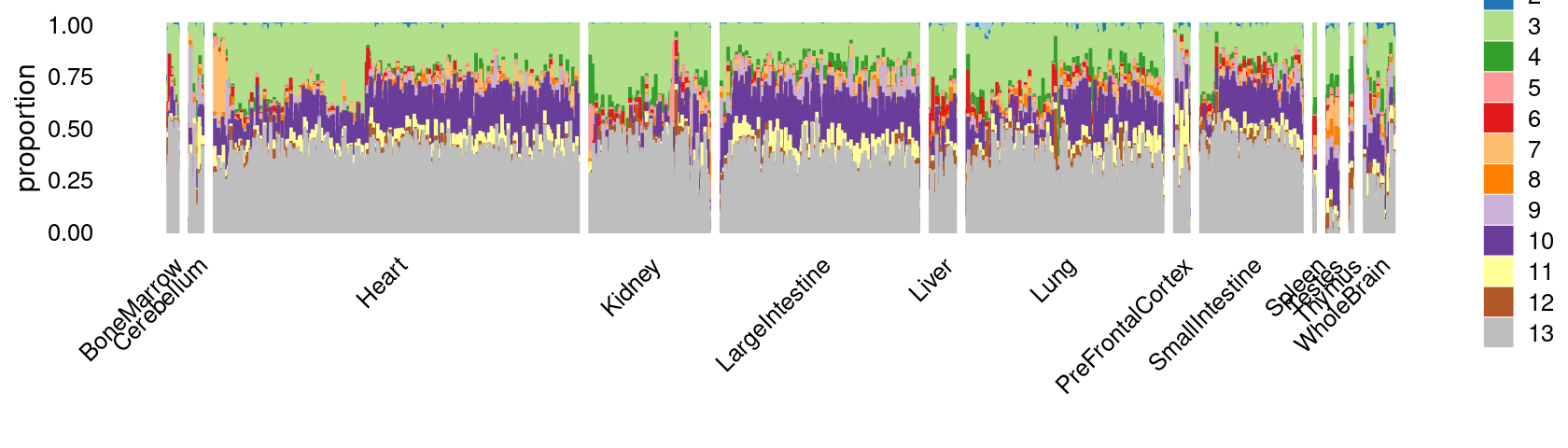
| Version | Author | Date |
|---|---|---|
| 96392bf | kevinlkx | 2020-12-02 |
breaks <- c(0,1,5,10,100,Inf)

fit.c6 <- select(poisson2multinom(fit),loadings = rows.c6)
p.pca.c6 <- pca_plot(fit.c6,fill = "none")
p.pca.hexbin.c6 <- pca_hexbin_plot(fit.c6,breaks = breaks) + guides(fill = "none")
plot_grid(p.pca.c6, p.pca.hexbin.c6)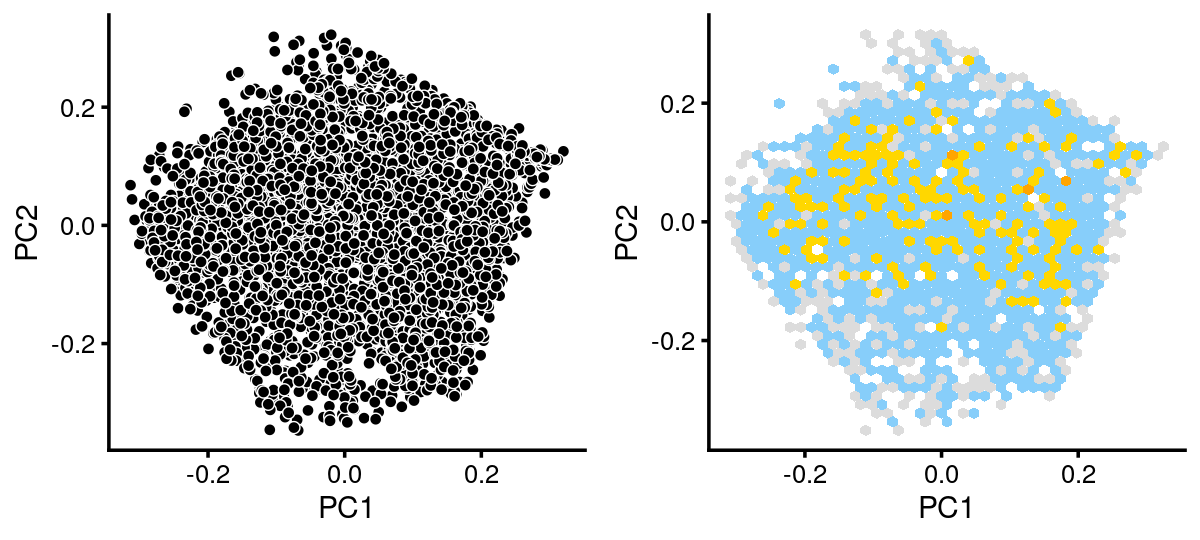
| Version | Author | Date |
|---|---|---|
| 96392bf | kevinlkx | 2020-12-02 |
The variation in PCs 1 and 2 is mostly produced by topics 3,9,10,11,13
p.pca.c6.topics <- pca_plot(fit.c6,k = c(3,9,10,11,13))
print(p.pca.c6.topics)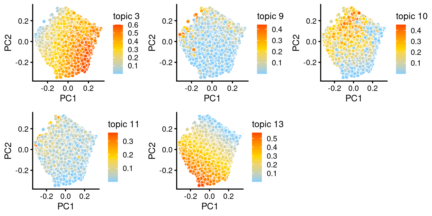
print(table(as.character(samples[rows.c6, "tissue"])))

print(table(as.character(samples[rows.c6, "cell_label"])))

p.pca.c6.tissue <- labeled_pca_plot(fit.c6,1:2,samples[rows.c6, "tissue"],font_size = 7,
                       colors = colors_tissues, legend_label = "tissue")
p.pca.c6.cell <- labeled_pca_plot(fit.c6,1:2,samples[rows.c6, "cell_label"],font_size = 7,
                        legend_label = "cell_label")
plot_grid(p.pca.c6.tissue,p.pca.c6.cell,rel_widths = c(8,11))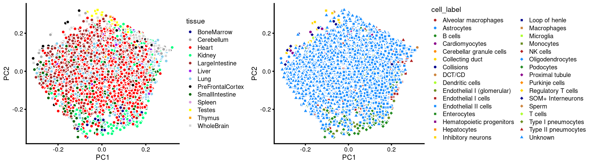
| Version | Author | Date |
|---|---|---|
| 96392bf | kevinlkx | 2020-12-02 |
#
#       BoneMarrow       Cerebellum            Heart           Kidney
#               33               44             1225              402
#   LargeIntestine            Liver             Lung PreFrontalCortex
#              665               84              659               48
#   SmallIntestine           Spleen           Testes           Thymus
#              341                5               37                9
#       WholeBrain
#               99
#
#       Alveolar macrophages                 Astrocytes
#                          2                         11
#                    B cells             Cardiomyocytes
#                          3                         42
#   Cerebellar granule cells            Collecting duct
#                          3                         10
#                 Collisions                     DCT/CD
#                         15                          1
#            Dendritic cells Endothelial I (glomerular)
#                          2                        158
#        Endothelial I cells       Endothelial II cells
#                        438                        574
#                Enterocytes  Hematopoietic progenitors
#                         11                          1
#                Hepatocytes         Inhibitory neurons
#                          5                         27
#              Loop of henle                Macrophages
#                          8                         14
#                  Microglia                  Monocytes
#                          3                          1
#                   NK cells           Oligodendrocytes
#                          1                          1
#                  Podocytes            Proximal tubule
#                        113                         16
#             Purkinje cells         Regulatory T cells
#                          2                          1
#          SOM+ Interneurons                      Sperm
#                          8                          1
#                    T cells         Type I pneumocytes
#                          7                          3
#        Type II pneumocytes                    Unknown
#                         14                       2155
zoom into cluster c9
rows.c9 <- which(samples$cluster_kmeans == "c9")Structure plot of c9 cluster: Group samples by tissue labels first, then by cell labels
tissue_labels_c9 <- as.factor(as.character(samples[rows.c9, "tissue"]))
cell_labels_c9 <- as.factor(as.character(samples[rows.c9, "cell_label"]))

p.structure.c9.1 <- structure_plot(select(poisson2multinom(fit),loadings = rows.c9),
                     grouping = tissue_labels_c9,
                     rows = order(cell_labels_c9),
                     n = Inf,gap = 40,
                     perplexity = 50,topics = 1:13,colors = colors_topics,
                     num_threads = 4,verbose = FALSE)
print(p.structure.c9.1)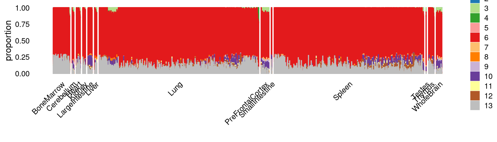
breaks <- c(0,1,5,10,100,Inf)
fit.c9 <- select(poisson2multinom(fit),loadings = rows.c9)
p.pca.c9 <- pca_plot(fit.c9,fill = "none")
p.pca.hexbin.c9 <- pca_hexbin_plot(fit.c9,breaks = breaks) + guides(fill = "none")
plot_grid(p.pca.c9, p.pca.hexbin.c9)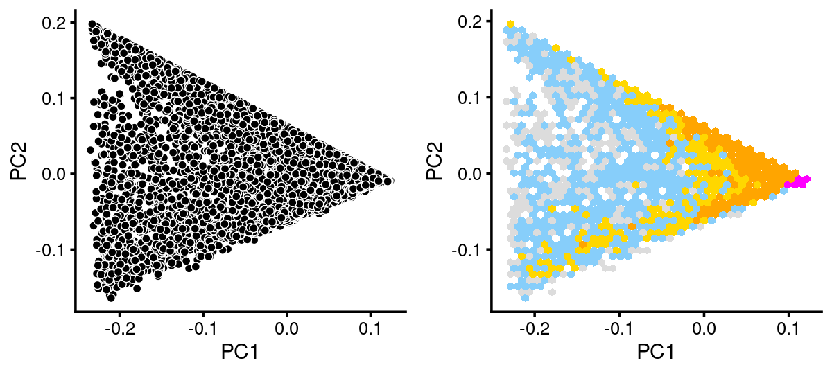 The variation in PCs 1 and 2 is mostly produced by topics 6,10,13.
p.pca.c9.topics <- pca_plot(fit.c9,k = c(6,10,13))
print(p.pca.c9.topics)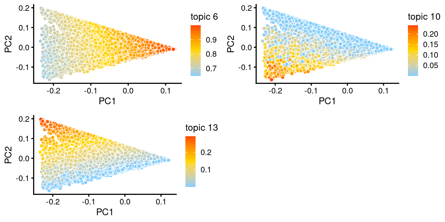
print(table(as.character(samples[rows.c9, "tissue"])))

print(table(as.character(samples[rows.c9, "cell_label"])))

p.pca.c9.tissue <- labeled_pca_plot(fit.c9,1:2,samples[rows.c9, "tissue"],font_size = 7,
                       colors = colors_tissues, legend_label = "tissue")
p.pca.c9.cell <- labeled_pca_plot(fit.c9,1:2,samples[rows.c9, "cell_label"],font_size = 7,
                        legend_label = "cell_label")
plot_grid(p.pca.c9.tissue,p.pca.c9.cell,rel_widths = c(8,11))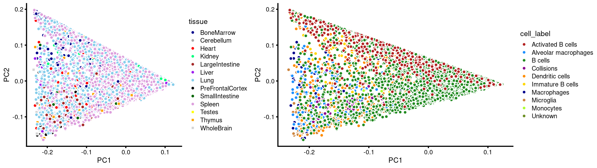
#
#       BoneMarrow       Cerebellum            Heart           Kidney
#              276               30               68               48
#   LargeIntestine            Liver             Lung PreFrontalCortex
#               71               39             2678              131
#   SmallIntestine           Spleen           Testes           Thymus
#                9             2510                2               90
#       WholeBrain
#               93
#
#    Activated B cells Alveolar macrophages              B cells
#                  331                  185                 4616
#           Collisions      Dendritic cells     Immature B cells
#                   44                  424                   68
#          Macrophages            Microglia            Monocytes
#                  127                  226                    9
#              Unknown
#                   15
sessionInfo()
# R version 3.6.1 (2019-07-05)
# Platform: x86_64-pc-linux-gnu (64-bit)
# Running under: Scientific Linux 7.4 (Nitrogen)
#
# Matrix products: default
# BLAS/LAPACK: /software/openblas-0.2.19-el7-x86_64/lib/libopenblas_haswellp-r0.2.19.so
#
# locale:
#  [1] LC_CTYPE=en_US.UTF-8       LC_NUMERIC=C
#  [3] LC_TIME=en_US.UTF-8        LC_COLLATE=en_US.UTF-8
#  [5] LC_MONETARY=en_US.UTF-8    LC_MESSAGES=en_US.UTF-8
#  [7] LC_PAPER=en_US.UTF-8       LC_NAME=C
#  [9] LC_ADDRESS=C               LC_TELEPHONE=C
# [11] LC_MEASUREMENT=en_US.UTF-8 LC_IDENTIFICATION=C
#
# attached base packages:
# [1] stats     graphics  grDevices utils     datasets  methods   base
#
# other attached packages:
# [1] RColorBrewer_1.1-2 plyr_1.8.6         fastTopics_0.3-180 cowplot_1.1.0
# [5] ggplot2_3.3.2      dplyr_1.0.2        Matrix_1.2-18      workflowr_1.6.2
#
# loaded via a namespace (and not attached):
#  [1] ggrepel_0.8.2      Rcpp_1.0.5         lattice_0.20-41    tidyr_1.1.2
#  [5] prettyunits_1.1.1  rprojroot_1.3-2    digest_0.6.27      R6_2.5.0
#  [9] backports_1.2.0    MatrixModels_0.4-1 evaluate_0.14      coda_0.19-3
# [13] httr_1.4.2         pillar_1.4.7       rlang_0.4.8        progress_1.2.2
# [17] lazyeval_0.2.2     data.table_1.13.2  irlba_2.3.3        SparseM_1.77
# [21] whisker_0.4        hexbin_1.28.1      rmarkdown_2.5      labeling_0.4.2
# [25] Rtsne_0.15         stringr_1.4.0      htmlwidgets_1.5.2  munsell_0.5.0
# [29] compiler_3.6.1     httpuv_1.5.4       xfun_0.19          pkgconfig_2.0.3
# [33] mcmc_0.9-7         htmltools_0.5.0    tidyselect_1.1.0   tibble_3.0.4
# [37] quadprog_1.5-7     viridisLite_0.3.0  crayon_1.3.4       withr_2.3.0
# [41] later_1.1.0.1      MASS_7.3-53        grid_3.6.1         jsonlite_1.6
# [45] gtable_0.3.0       lifecycle_0.2.0    git2r_0.27.1       magrittr_1.5
# [49] scales_1.1.1       RcppParallel_5.0.2 stringi_1.5.3      farver_2.0.3
# [53] fs_1.3.1           promises_1.1.1     ellipsis_0.3.1     generics_0.0.2
# [57] vctrs_0.3.5        tools_3.6.1        glue_1.4.2         purrr_0.3.4
# [61] hms_0.5.3          yaml_2.2.0         colorspace_2.0-0   plotly_4.9.0
# [65] knitr_1.30         quantreg_5.41      MCMCpack_1.4-4