Clustering Lareau et al (2019) bone marrow data using topic proportions with K = 13
Kaixuan Luo
Last updated: 2020-10-22
Checks: 7 0
Knit directory: scATACseq-topics/
This reproducible R Markdown analysis was created with workflowr (version 1.6.2). The Checks tab describes the reproducibility checks that were applied when the results were created. The Past versions tab lists the development history.
Great! Since the R Markdown file has been committed to the Git repository, you know the exact version of the code that produced these results.
Great job! The global environment was empty. Objects defined in the global environment can affect the analysis in your R Markdown file in unknown ways. For reproduciblity it’s best to always run the code in an empty environment.
The command set.seed(20200729) was run prior to running the code in the R Markdown file. Setting a seed ensures that any results that rely on randomness, e.g. subsampling or permutations, are reproducible.
Great job! Recording the operating system, R version, and package versions is critical for reproducibility.
Nice! There were no cached chunks for this analysis, so you can be confident that you successfully produced the results during this run.
Great job! Using relative paths to the files within your workflowr project makes it easier to run your code on other machines.
Great! You are using Git for version control. Tracking code development and connecting the code version to the results is critical for reproducibility.
The results in this page were generated with repository version f9a1ac4. See the Past versions tab to see a history of the changes made to the R Markdown and HTML files.
Note that you need to be careful to ensure that all relevant files for the analysis have been committed to Git prior to generating the results (you can use wflow_publish or wflow_git_commit). workflowr only checks the R Markdown file, but you know if there are other scripts or data files that it depends on. Below is the status of the Git repository when the results were generated:
Ignored files:
    Ignored:    .Rhistory
    Ignored:    .Rproj.user/

Untracked files:
    Untracked:  analysis/clusters_pca_structure_Cusanovich2018.Rmd

Unstaged changes:
    Modified:   analysis/plots_Lareau2019_bonemarrow.Rmd
    Modified:   code/plots.R
    Modified:   scripts/fit_all_models_Lareau2019.sh
Note that any generated files, e.g. HTML, png, CSS, etc., are not included in this status report because it is ok for generated content to have uncommitted changes.
These are the previous versions of the repository in which changes were made to the R Markdown (analysis/clusters_Lareau2019_bonemarrow_k13.Rmd) and HTML (docs/clusters_Lareau2019_bonemarrow_k13.html) files. If you’ve configured a remote Git repository (see ?wflow_git_remote), click on the hyperlinks in the table below to view the files as they were in that past version.
| File | Version | Author | Date | Message |
|---|---|---|---|---|
| Rmd | f9a1ac4 | kevinlkx | 2020-10-22 | add more descriptions about the study design |
| html | 2d1a85b | kevinlkx | 2020-10-21 | Build site. |
| Rmd | 9058074 | kevinlkx | 2020-10-21 | add interpretations for clusters |
| html | fa7f769 | kevinlkx | 2020-10-21 | Build site. |
| Rmd | 4b016ee | kevinlkx | 2020-10-21 | wflow_publish(“analysis/clusters_Lareau2019_bonemarrow_k13.Rmd”) |
| html | 697d54e | kevinlkx | 2020-10-21 | Build site. |
| Rmd | cad6c07 | kevinlkx | 2020-10-21 | clustering cells based on topic proportions from K = 13 topics |
Here we explore the structure in the Lareau et al (2019) human bone marrow scATAC-seq data inferred from the multinomial topic model with \(k = 13\).
Load packages and some functions used in this analysis.
library(Matrix)
library(dplyr)
library(ggplot2)
library(cowplot)
library(fastTopics)
source("code/plots.R")
The study used dsciATAC-seq to profile bone marrow mononuclear cells (BMMCs) from two human donors before (untreated controls) and after stimulation.
Resting condition
The reference map of 60,495 resting cells (untreated controls) revealed the major lineages of hematopoietic differentiation de novo.
Load the data in resting condition
data.dir <- "/project2/mstephens/kevinluo/scATACseq-topics/data/Lareau_2019/bone_marrow/processed_data/"
load(file.path(data.dir, "Lareau_2019_bonemarrow_resting.RData"))
cat(sprintf("%d x %d counts matrix.\n",nrow(counts),ncol(counts)))
rm(counts)
samples$Cluster <- as.factor(samples$Cluster)
# 60495 x 146860 counts matrix.
Plot PCs of the topic proportions
We first use PCA to explore the structure inferred from the multinomial topic model with \(k = 13\):
out.dir <- "/project2/mstephens/kevinluo/scATACseq-topics/output/Lareau_2019/Lareau_2019_bonemarrow_resting"
fit <- readRDS(file.path(out.dir, "/fit-Lareau2019_bonemarrow_resting-scd-ex-k=13.rds"))$fit
Plot PCs of the topic proportions.
p.pca1.1 <- pca_plot(poisson2multinom(fit),pcs = 1:2,fill = "none")
p.pca1.2 <- pca_plot(poisson2multinom(fit),pcs = 3:4,fill = "none")
p.pca1.3 <- pca_plot(poisson2multinom(fit),pcs = 5:6,fill = "none")
p.pca1.4 <- pca_plot(poisson2multinom(fit),pcs = 7:8,fill = "none")
p.pca1.5 <- pca_plot(poisson2multinom(fit),pcs = 9:10,fill = "none")
p.pca1.6 <- pca_plot(poisson2multinom(fit),pcs = 11:12,fill = "none")

plot_grid(p.pca1.1,p.pca1.2,p.pca1.3,p.pca1.4,p.pca1.5,p.pca1.6)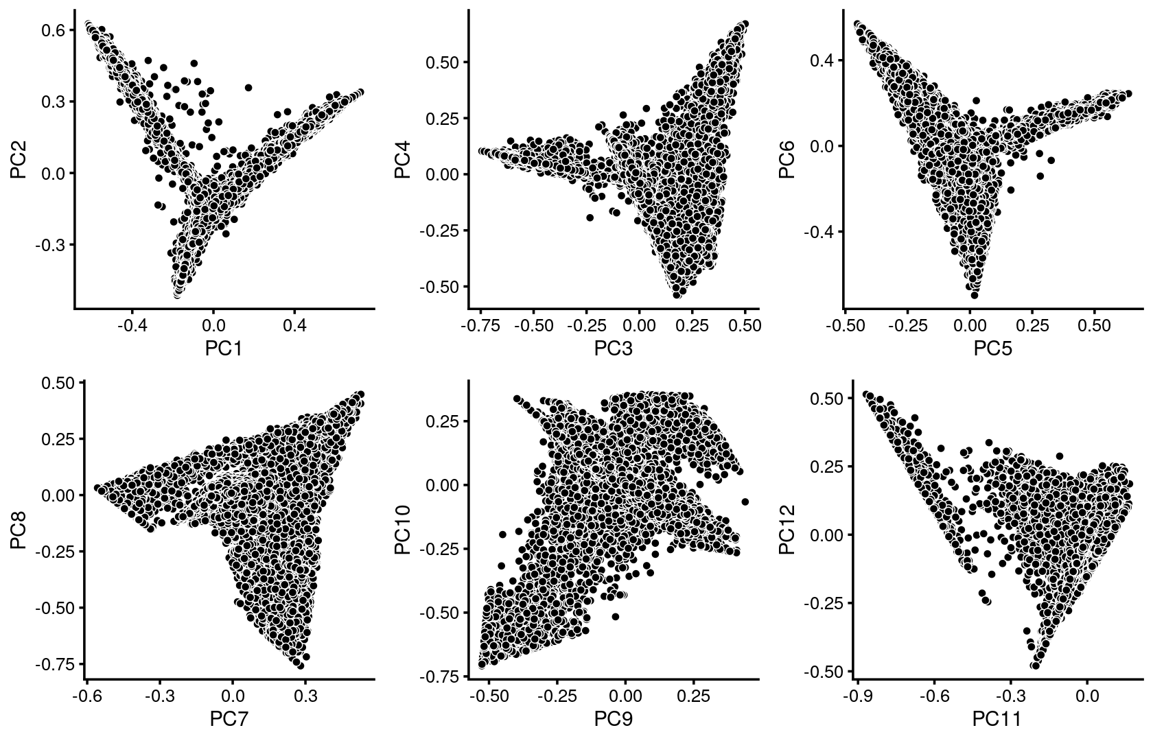
| Version | Author | Date |
|---|---|---|
| 697d54e | kevinlkx | 2020-10-21 |
Some of the structure is more evident from “hexbin” plots showing the density of the points.
breaks <- c(0,1,5,10,100,Inf)
p.pca2.1 <- pca_hexbin_plot(poisson2multinom(fit), pcs = 1:2, breaks = breaks) + guides(fill = "none")
p.pca2.2 <- pca_hexbin_plot(poisson2multinom(fit), pcs = 3:4, breaks = breaks) + guides(fill = "none")
p.pca2.3 <- pca_hexbin_plot(poisson2multinom(fit), pcs = 5:6, breaks = breaks) + guides(fill = "none")
p.pca2.4 <- pca_hexbin_plot(poisson2multinom(fit), pcs = 7:8, breaks = breaks) + guides(fill = "none")
p.pca2.5 <- pca_hexbin_plot(poisson2multinom(fit), pcs = 9:10, breaks = breaks) + guides(fill = "none")
p.pca2.6 <- pca_hexbin_plot(poisson2multinom(fit), pcs = 11:12, breaks = breaks) + guides(fill = "none")

plot_grid(p.pca2.1,p.pca2.2,p.pca2.3,p.pca2.4,p.pca2.5,p.pca2.6)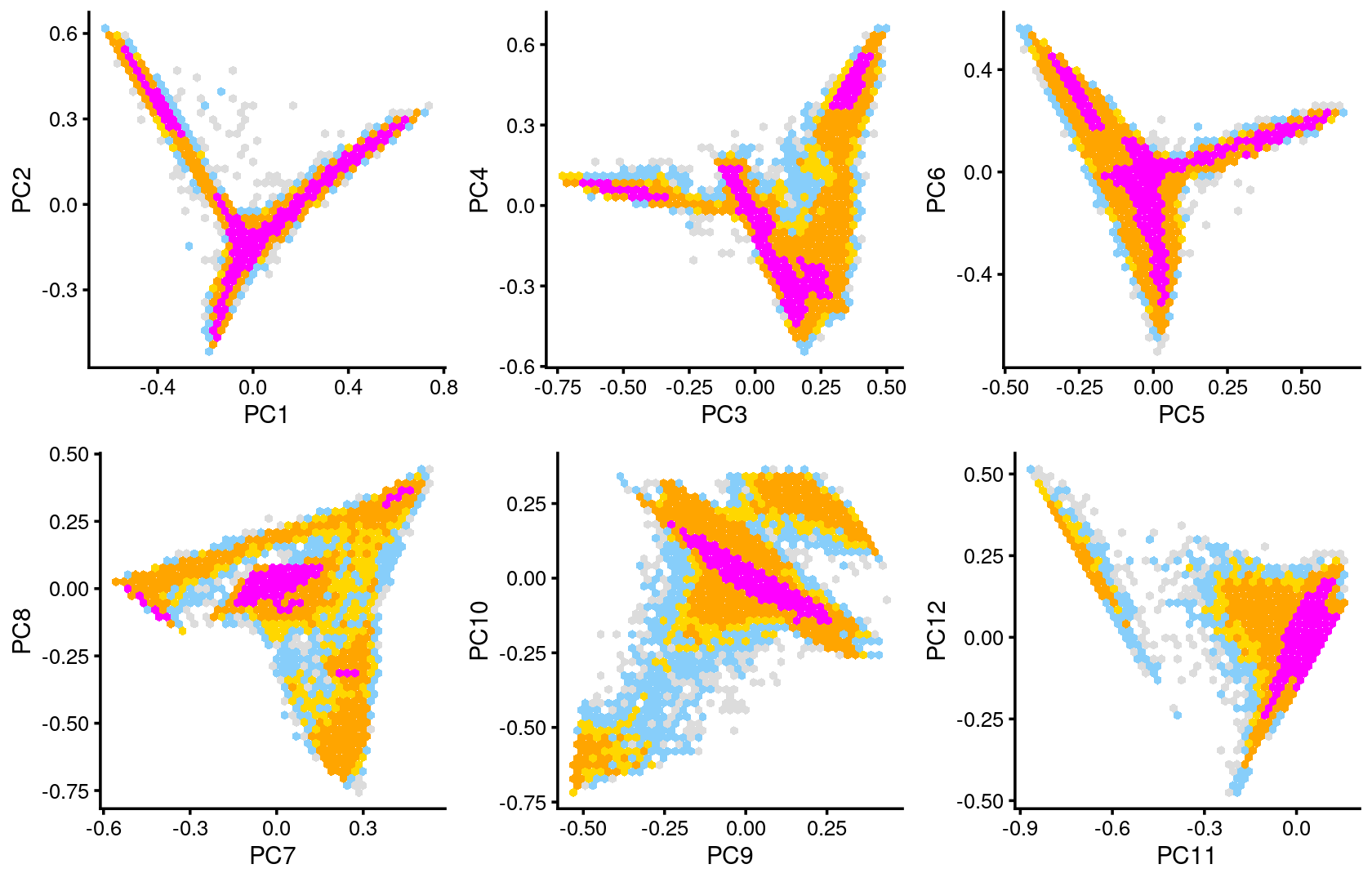
| Version | Author | Date |
|---|---|---|
| 697d54e | kevinlkx | 2020-10-21 |
Layer the cell labels onto the PC plots
The authors projected the untreated BMMCs onto hematopoietic development trajectories using a reference-guided approach. They predicted cell labels given the bulk sorted hematopoietic ATAC-seq profiles, and then identified 15 distinct clusters from the 60,495 resting cells, which recapitulated the major constitutive cell types in the human hematopoietic system.
Here, we layer the predicted cell labels onto the PC plots.
p.pca3.1 <- labeled_pca_plot(fit,1:2,samples$Cluster,font_size = 7,
                       legend_label = "Cell labels")
p.pca3.2 <- labeled_pca_plot(fit,3:4,samples$Cluster,font_size = 7,
                       legend_label = "Cell labels")
p.pca3.3 <- labeled_pca_plot(fit,5:6,samples$Cluster,font_size = 7,
                       legend_label = "Cell labels")
p.pca3.4 <- labeled_pca_plot(fit,7:8,samples$Cluster,font_size = 7,
                       legend_label = "Cell labels")
p.pca3.5 <- labeled_pca_plot(fit,9:10,samples$Cluster,font_size = 7,
                       legend_label = "Cell labels")
p.pca3.6 <- labeled_pca_plot(fit,11:12,samples$Cluster,font_size = 7,
                       legend_label = "Cell labels")
plot_grid(p.pca3.1,p.pca3.2,p.pca3.3,p.pca3.4,p.pca3.5,p.pca3.6)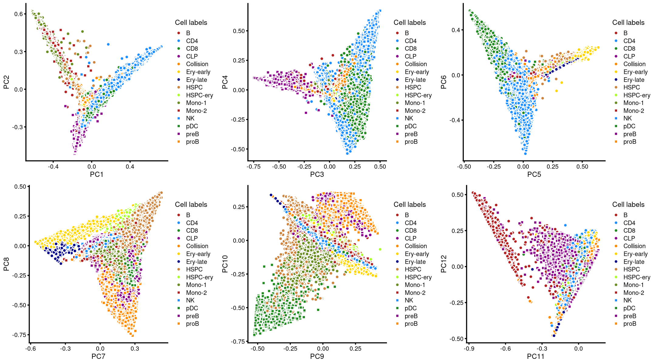
| Version | Author | Date |
|---|---|---|
| 697d54e | kevinlkx | 2020-10-21 |
Visualize by structure plot grouped by cell labels.
set.seed(10)
colors_topics <- c("#a6cee3","#1f78b4","#b2df8a","#33a02c","#fb9a99","#e31a1c",
                   "#fdbf6f","#ff7f00","#cab2d6","#6a3d9a","#ffff99","#b15928",
                   "gray")
rows <- sample(nrow(fit$L),4000)
samples$Cluster <- as.factor(samples$Cluster)

p.structure.1 <- structure_plot(select(poisson2multinom(fit),loadings = rows),
                     grouping = samples[rows, "Cluster"],n = Inf,gap = 20,
                     perplexity = 50,topics = 1:13,colors = colors_topics,
                     num_threads = 4,verbose = FALSE)
# Perplexity automatically changed to 17 because original setting of 50 was too large for the number of samples (56)
# Perplexity automatically changed to 6 because original setting of 50 was too large for the number of samples (22)
# Perplexity automatically changed to 6 because original setting of 50 was too large for the number of samples (24)
# Perplexity automatically changed to 22 because original setting of 50 was too large for the number of samples (71)
# Perplexity automatically changed to 10 because original setting of 50 was too large for the number of samples (34)
# Perplexity automatically changed to 21 because original setting of 50 was too large for the number of samples (69)
# Perplexity automatically changed to 32 because original setting of 50 was too large for the number of samples (101)

print(p.structure.1)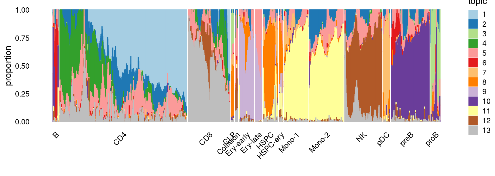
k-means clustering on topic proportions
Define clusters using k-means, and then create structure plot based on the clusters from k-means.
Define clusters using k-means with \(k = 10\):
set.seed(10)

clusters.10 <- factor(kmeans(poisson2multinom(fit)$L,centers = 10)$cluster)
print(sort(table(clusters.10),decreasing = TRUE))
# clusters.10
#    10     1     3     6     4     5     7     2     8     9
# 10753 10175  7857  6055  5803  5090  4839  3593  3339  2991
Structure plot based on k-means clusters
colors_topics <- c("#a6cee3","#1f78b4","#b2df8a","#33a02c","#fb9a99","#e31a1c",
                   "#fdbf6f","#ff7f00","#cab2d6","#6a3d9a","#ffff99","#b15928",
                   "gray")
rows <- sample(nrow(fit$L),4000)

p.structure.2 <- structure_plot(select(poisson2multinom(fit),loadings = rows),
                     grouping = clusters.10[rows],n = Inf,gap = 20,
                     perplexity = 50,topics = 1:13,colors = colors_topics,
                     num_threads = 4,verbose = FALSE)
print(p.structure.2)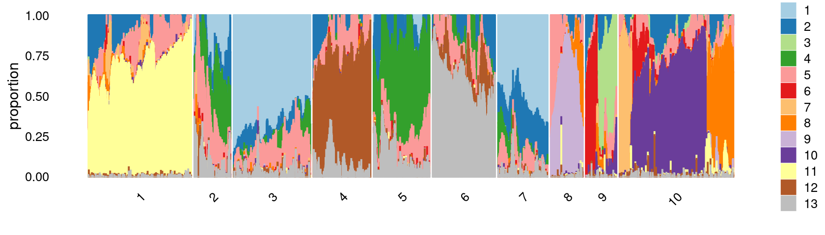
| Version | Author | Date |
|---|---|---|
| 697d54e | kevinlkx | 2020-10-21 |
Define clusters using k-means with \(k = 12\):
set.seed(10)

clusters.12 <- factor(kmeans(poisson2multinom(fit)$L,centers = 12)$cluster)
print(sort(table(clusters.12),decreasing = TRUE))
# clusters.12
#     3     1    12     5     8    10     4     7     2     6    11     9
# 12075 10014  6866  5978  5395  5045  3829  3667  3173  2147  1412   894
Structure plot based on k-means clusters
colors_topics <- c("#a6cee3","#1f78b4","#b2df8a","#33a02c","#fb9a99","#e31a1c",
                   "#fdbf6f","#ff7f00","#cab2d6","#6a3d9a","#ffff99","#b15928",
                   "gray")
rows <- sample(nrow(fit$L),4000)

p.structure.3 <- structure_plot(select(poisson2multinom(fit),loadings = rows),
                     grouping = clusters.12[rows],n = Inf,gap = 20,
                     perplexity = 50,topics = 1:13,colors = colors_topics,
                     num_threads = 4,verbose = FALSE)
# Perplexity automatically changed to 44 because original setting of 50 was too large for the number of samples (136)
# Perplexity automatically changed to 18 because original setting of 50 was too large for the number of samples (60)
# Perplexity automatically changed to 25 because original setting of 50 was too large for the number of samples (79)
print(p.structure.3)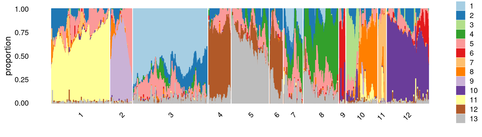
| Version | Author | Date |
|---|---|---|
| 697d54e | kevinlkx | 2020-10-21 |
Refine clusters
We then further refine the clusters based on k-means result with \(k = 12\): merge clusters 4 and 6; (maybe also merge clusters 7 and 8).
clusters.merged <- clusters.12
clusters.merged[clusters.12 %in% c(4,6)] <- 4
# clusters.merged[clusters.12 %in% c(7,8)] <- 7
clusters.merged <- factor(clusters.merged, labels = paste0("c", c(1:length(unique(clusters.merged)))))
print(sort(table(clusters.merged),decreasing = TRUE))

samples$cluster_kmeans <- clusters.merged
# clusters.merged
#    c3    c1   c11    c5    c4    c7    c9    c6    c2   c10    c8
# 12075 10014  6866  5978  5976  5395  5045  3667  3173  1412   894
colors_topics <- c("#a6cee3","#1f78b4","#b2df8a","#33a02c","#fb9a99","#e31a1c",
"#fdbf6f","#ff7f00","#cab2d6","#6a3d9a","#ffff99","#b15928",
"gray")
rows <- sample(nrow(fit$L),4000)
p.structure.refined <- structure_plot(select(poisson2multinom(fit),loadings = rows),
grouping = clusters.merged[rows],n = Inf,gap = 20,
perplexity = 50,topics = 1:13,colors = colors_topics,
num_threads = 4,verbose = FALSE)
# Perplexity automatically changed to 18 because original setting of 50 was too large for the number of samples (59)
# Perplexity automatically changed to 26 because original setting of 50 was too large for the number of samples (84)
print(p.structure.refined)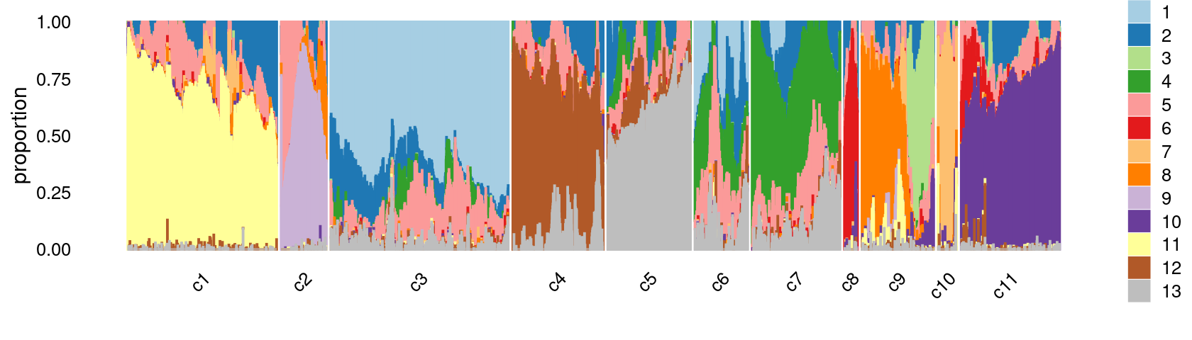
| Version | Author | Date |
|---|---|---|
| 697d54e | kevinlkx | 2020-10-21 |
The clusters defined by k-means on topic proportions reasonably identify the clusters shown in the PCA hexbin plots (below).
p.pca.4.1 <- labeled_pca_plot(fit,1:2,samples$cluster_kmeans,font_size = 7,
                       legend_label = "cluster_kmeans")
p.pca.4.2 <- labeled_pca_plot(fit,3:4,samples$cluster_kmeans,font_size = 7,
                       legend_label = "cluster_kmeans")
p.pca.4.3 <- labeled_pca_plot(fit,5:6,samples$cluster_kmeans,font_size = 7,
                       legend_label = "cluster_kmeans")
p.pca.4.4 <- labeled_pca_plot(fit,7:8,samples$cluster_kmeans,font_size = 7,
                       legend_label = "cluster_kmeans")
p.pca.4.5 <- labeled_pca_plot(fit,9:10,samples$cluster_kmeans,font_size = 7,
                       legend_label = "cluster_kmeans")
p.pca.4.6 <- labeled_pca_plot(fit,11:12,samples$cluster_kmeans,font_size = 7,
                       legend_label = "cluster_kmeans")
plot_grid(p.pca.4.1,p.pca.4.2,p.pca.4.3,p.pca.4.4,p.pca.4.5,p.pca.4.6)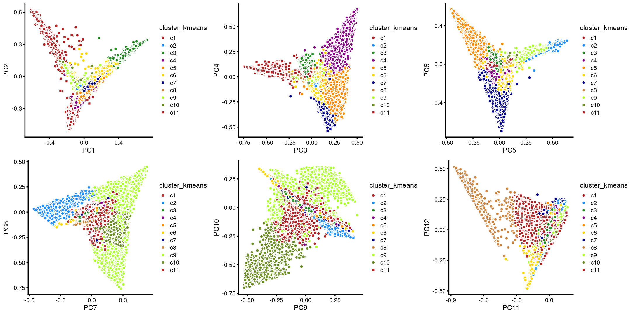
| Version | Author | Date |
|---|---|---|
| 697d54e | kevinlkx | 2020-10-21 |
plot_grid(p.pca2.1,p.pca2.2,p.pca2.3,p.pca2.4,p.pca2.5,p.pca2.6)
| Version | Author | Date |
|---|---|---|
| 697d54e | kevinlkx | 2020-10-21 |
We then label the cells in each cluster with the known cell labels.
Cell labels:
samples$Cluster <- as.factor(samples$Cluster)
cat(length(levels(samples$Cluster)), "cell labels. \n")
table(samples$Cluster)
# 15 cell labels.
#
#         B       CD4       CD8       CLP Collision Ery-early  Ery-late      HSPC
#      1001     20378      6647       411       271      2176      1174      2536
#  HSPC-ery    Mono-1    Mono-2        NK       pDC      preB      proB
#       479      3913      6012      5741      1218      6658      1880
Plot the distribution of cell labels by clusters.
Stacked barplot for the counts of cell labels by clusters:
library(plyr);library(dplyr)
# ------------------------------------------------------------------------------
# You have loaded plyr after dplyr - this is likely to cause problems.
# If you need functions from both plyr and dplyr, please load plyr first, then dplyr:
# library(plyr); library(dplyr)
# ------------------------------------------------------------------------------
#
# Attaching package: 'plyr'
# The following objects are masked from 'package:dplyr':
#
#     arrange, count, desc, failwith, id, mutate, rename, summarise,
#     summarize
library(RColorBrewer)

freq_cluster_tissue <- count(samples, vars=c("cluster_kmeans","Cluster"))
n_colors <- length(levels(samples$Cluster))
colors_labels <- colorRampPalette(brewer.pal(9, "Set1"))(n_colors)

# stacked barplot for the counts of cell labels by clusters
p.barplot.1 <- ggplot(freq_cluster_tissue, aes(fill=Cluster, y=freq, x=cluster_kmeans)) +
  geom_bar(position="stack", stat="identity") +
  theme_classic() + xlab("Cluster") + ylab("Number of cells") +
  scale_fill_manual(values = colors_labels) +
  guides(fill=guide_legend(ncol=2)) +
  theme(
  legend.title = element_text(size = 10),
  legend.text = element_text(size = 8)
  )
print(p.barplot.1)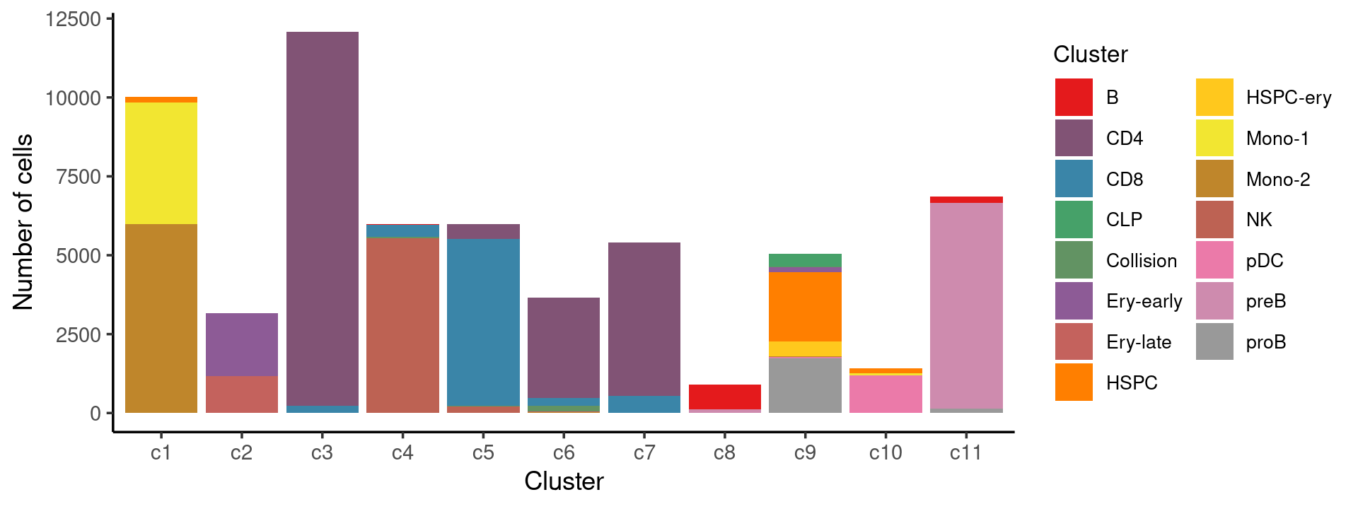
| Version | Author | Date |
|---|---|---|
| 697d54e | kevinlkx | 2020-10-21 |
Percent stacked barplot for the counts of cell labels by clusters:
freq_cluster_tissue <- count(samples, vars=c("cluster_kmeans","Cluster"))
n_colors <- length(levels(samples$Cluster))
colors_labels <- colorRampPalette(brewer.pal(9, "Set1"))(n_colors)

p.barplot.2 <- ggplot(freq_cluster_tissue, aes(fill=Cluster, y=freq, x=cluster_kmeans)) +
  geom_bar(position="fill", stat="identity") +
  theme_classic() + xlab("Cluster") + ylab("Proportion of cells") +
  scale_fill_manual(values = colors_labels) +
  guides(fill=guide_legend(ncol=2)) +
  theme(
  legend.title = element_text(size = 10),
  legend.text = element_text(size = 8)
  )
print(p.barplot.2)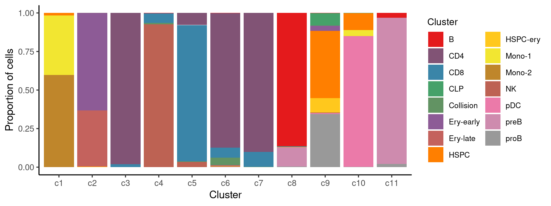
| Version | Author | Date |
|---|---|---|
| 697d54e | kevinlkx | 2020-10-21 |
We can see a few clusters are dominated by one major cell type: * cells in cluster c3 are primarily CD4 cells; * cells in cluster c4 are primarily NK cells; * cells in cluster c5 are primarily CD8 cells; * the majority of cells in cluster c6 and c7 are CD4 cells; * the majority of cells in cluster c8 are CD4 cells (and B cells); * the majority of cells in cluster c10 are pDC cells (and HSPC cells); * the majority of cells in cluster c11 are preB cells.
Some clusters are combinations of related cell types: * cells in cluster c1 are a combination of Mono-1 and Mono-2 cells; * cells in cluster c2 are a combination of Ery-early and Ery-late cells;
Cluster c9 is more heterogeneous with HSPC, HSPC-ery, proB, and CLP cells.
freq_cluster_cells <- with(samples,table(Cluster,cluster_kmeans))
print(freq_cluster_cells)
#            cluster_kmeans
# Cluster        c1    c2    c3    c4    c5    c6    c7    c8    c9   c10   c11
#   B             0     0     0     9     0     8     0   773     3     0   208
#   CD4           0     2 11836    14   469  3192  4862     0     1     0     2
#   CD8           0     0   234   363  5289   240   520     1     0     0     0
#   CLP           0     0     0     0     0     0     0     0   410     1     0
#   Collision     2     1     4    54    18   181     7     2     2     0     0
#   Ery-early     0  2002     0     0     0     2     1     1   170     0     0
#   Ery-late      0  1157     0     0     0    16     0     1     0     0     0
#   HSPC        169     2     0     2     3     2     1     0  2202   155     0
#   HSPC-ery      1     7     0     0     0     5     0     1   465     0     0
#   Mono-1     3851     0     0     0     0     0     1     1     5    55     0
#   Mono-2     5990     0     0     3     0     8     0     0    11     0     0
#   NK            1     2     0  5531   196     8     1     0     2     0     0
#   pDC           0     0     1     0     0     0     0     0    18  1199     0
#   preB          0     0     0     0     3     5     2   110    19     0  6519
#   proB          0     0     0     0     0     0     0     4  1737     2   137
Stimulated condition
To characterize the response of each immune cell cluster to stimulation conditions, the authors explored the differences between the untreated control cells and ex vivo cultured and lipopolysaccharide (LPS)-stimulated BMMCs.
The authors used a k-nearest neighbor map to connect stimulated cells to control cells.
Load the data in stimulated condition
data.dir <- "/project2/mstephens/kevinluo/scATACseq-topics/data/Lareau_2019/bone_marrow/processed_data/"
load(file.path(data.dir, "Lareau_2019_bonemarrow_stimulated.RData"))
cat(sprintf("%d x %d counts matrix.\n",nrow(counts),ncol(counts)))
rm(counts)
samples$Cluster <- as.factor(samples$Cluster)
# 75968 x 146860 counts matrix.
Plot PCs of the topic proportions
We first use PCA to explore the structure inferred from the multinomial topic model with \(k = 13\):
out.dir <- "/project2/mstephens/kevinluo/scATACseq-topics/output/Lareau_2019/Lareau_2019_bonemarrow_stimulated"
fit <- readRDS(file.path(out.dir, "/fit-Lareau2019_bonemarrow_stimulated-scd-ex-k=13.rds"))$fit
Plot PCs of the topic proportions.
p.pca1.1 <- pca_plot(poisson2multinom(fit),pcs = 1:2,fill = "none")
p.pca1.2 <- pca_plot(poisson2multinom(fit),pcs = 3:4,fill = "none")
p.pca1.3 <- pca_plot(poisson2multinom(fit),pcs = 5:6,fill = "none")
p.pca1.4 <- pca_plot(poisson2multinom(fit),pcs = 7:8,fill = "none")
p.pca1.5 <- pca_plot(poisson2multinom(fit),pcs = 9:10,fill = "none")
p.pca1.6 <- pca_plot(poisson2multinom(fit),pcs = 11:12,fill = "none")

plot_grid(p.pca1.1,p.pca1.2,p.pca1.3,p.pca1.4,p.pca1.5,p.pca1.6)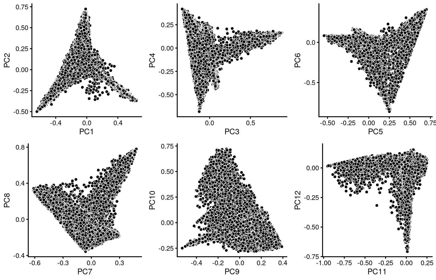
| Version | Author | Date |
|---|---|---|
| 697d54e | kevinlkx | 2020-10-21 |
Some of the structure is more evident from “hexbin” plots showing the density of the points.
breaks <- c(0,1,5,10,100,Inf)
p.pca2.1 <- pca_hexbin_plot(poisson2multinom(fit), pcs = 1:2, breaks = breaks) + guides(fill = "none")
p.pca2.2 <- pca_hexbin_plot(poisson2multinom(fit), pcs = 3:4, breaks = breaks) + guides(fill = "none")
p.pca2.3 <- pca_hexbin_plot(poisson2multinom(fit), pcs = 5:6, breaks = breaks) + guides(fill = "none")
p.pca2.4 <- pca_hexbin_plot(poisson2multinom(fit), pcs = 7:8, breaks = breaks) + guides(fill = "none")
p.pca2.5 <- pca_hexbin_plot(poisson2multinom(fit), pcs = 9:10, breaks = breaks) + guides(fill = "none")
p.pca2.6 <- pca_hexbin_plot(poisson2multinom(fit), pcs = 11:12, breaks = breaks) + guides(fill = "none")

plot_grid(p.pca2.1,p.pca2.2,p.pca2.3,p.pca2.4,p.pca2.5,p.pca2.6)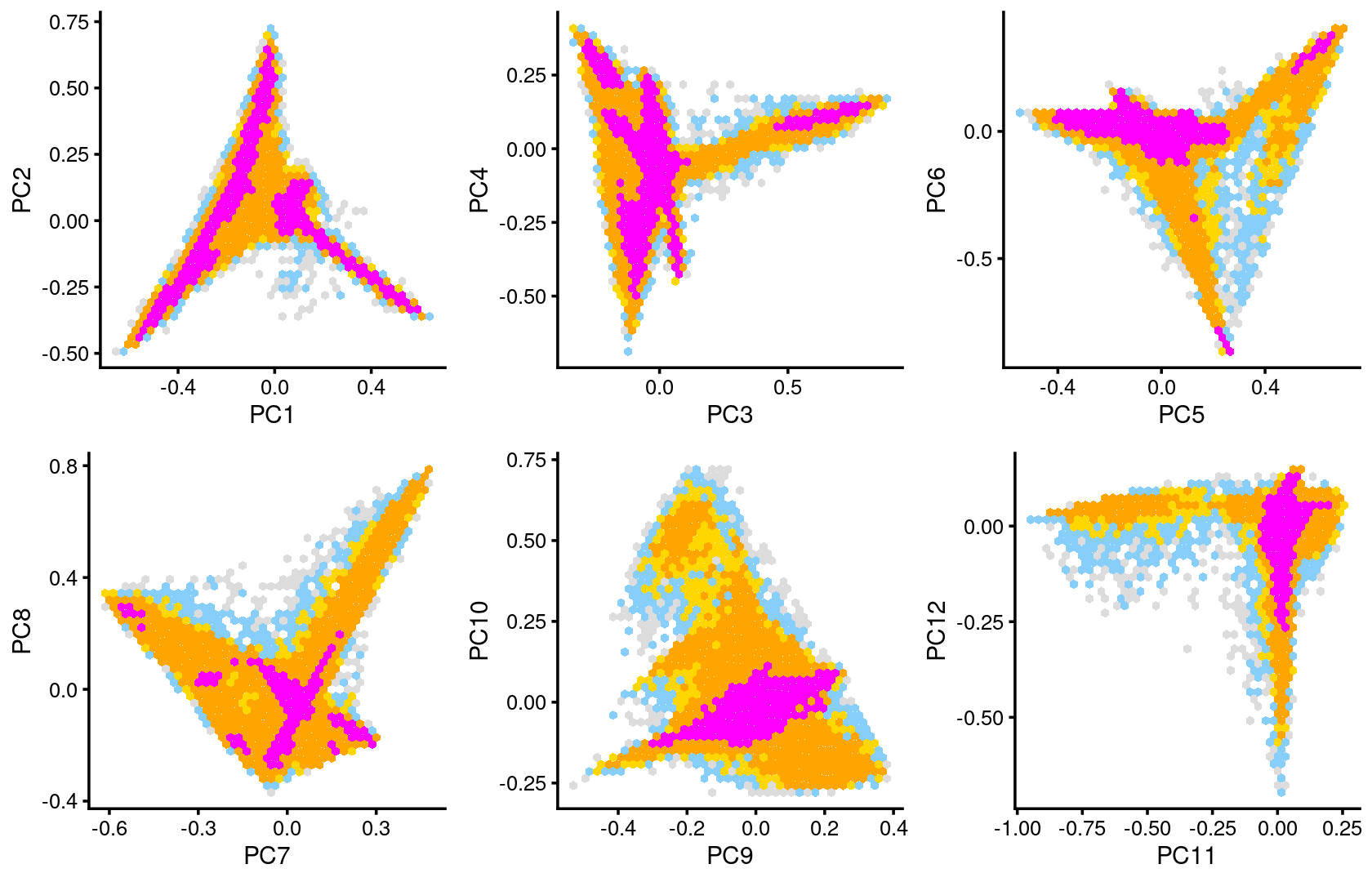
| Version | Author | Date |
|---|---|---|
| 697d54e | kevinlkx | 2020-10-21 |
Layer the cell labels onto the PC plots
We layer the predicted cell labels onto the PC plots.
p.pca3.1 <- labeled_pca_plot(fit,1:2,samples$Cluster,font_size = 7,
                       legend_label = "Cell labels")
p.pca3.2 <- labeled_pca_plot(fit,3:4,samples$Cluster,font_size = 7,
                       legend_label = "Cell labels")
p.pca3.3 <- labeled_pca_plot(fit,5:6,samples$Cluster,font_size = 7,
                       legend_label = "Cell labels")
p.pca3.4 <- labeled_pca_plot(fit,7:8,samples$Cluster,font_size = 7,
                       legend_label = "Cell labels")
p.pca3.5 <- labeled_pca_plot(fit,9:10,samples$Cluster,font_size = 7,
                       legend_label = "Cell labels")
p.pca3.6 <- labeled_pca_plot(fit,11:12,samples$Cluster,font_size = 7,
                       legend_label = "Cell labels")
plot_grid(p.pca3.1,p.pca3.2,p.pca3.3,p.pca3.4,p.pca3.5,p.pca3.6)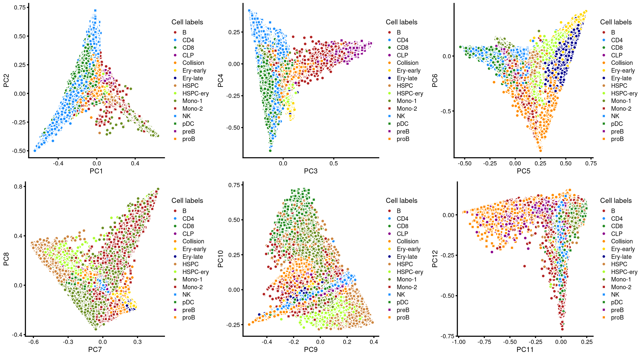
| Version | Author | Date |
|---|---|---|
| 697d54e | kevinlkx | 2020-10-21 |
Visualize by structure plot grouped by cell labels
set.seed(10)
colors_topics <- c("#a6cee3","#1f78b4","#b2df8a","#33a02c","#fb9a99","#e31a1c",
                   "#fdbf6f","#ff7f00","#cab2d6","#6a3d9a","#ffff99","#b15928",
                   "gray")
rows <- sample(nrow(fit$L),4000)
samples$Cluster <- as.factor(samples$Cluster)

p.structure.1 <- structure_plot(select(poisson2multinom(fit),loadings = rows),
                     grouping = samples[rows, "Cluster"],n = Inf,gap = 20,
                     perplexity = 50,topics = 1:13,colors = colors_topics,
                     num_threads = 4,verbose = FALSE)
# Perplexity automatically changed to 2 because original setting of 50 was too large for the number of samples (12)
# Perplexity automatically changed to 46 because original setting of 50 was too large for the number of samples (143)
# Perplexity automatically changed to 16 because original setting of 50 was too large for the number of samples (54)
# Perplexity automatically changed to 33 because original setting of 50 was too large for the number of samples (103)
# Perplexity automatically changed to 15 because original setting of 50 was too large for the number of samples (50)
# Perplexity automatically changed to 19 because original setting of 50 was too large for the number of samples (63)

print(p.structure.1)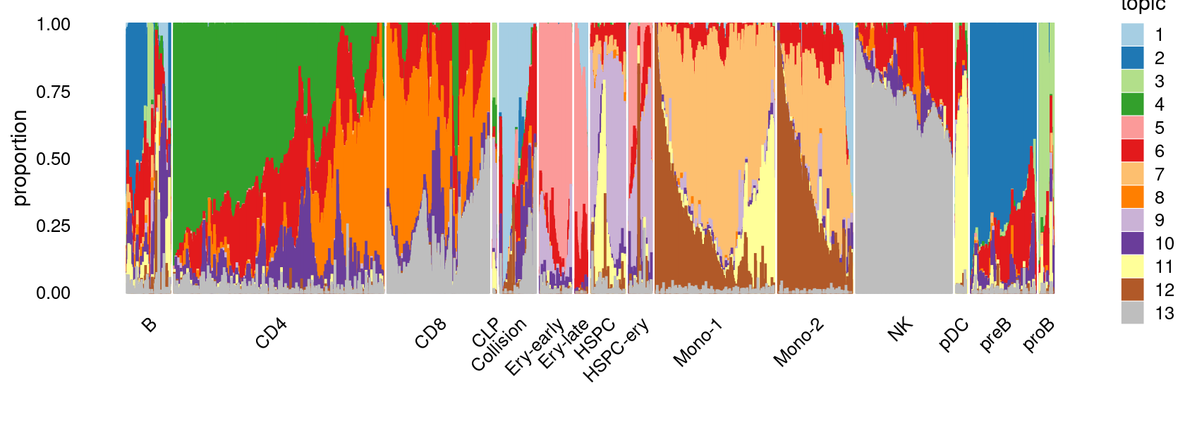
k-means clustering on topic proportions
Define clusters using k-means, and then create structure plot based on the clusters from k-means.
Define clusters using k-means with \(k = 10\):
set.seed(10)

clusters.10 <- factor(kmeans(poisson2multinom(fit)$L,centers = 10)$cluster)
print(sort(table(clusters.10),decreasing = TRUE))
# clusters.10
#     3     8     2    10     4     7     5     6     1     9
# 15209 11641  8174  8161  7711  6990  5376  4713  4556  3437
Structure plot based on k-means clusters
colors_topics <- c("#a6cee3","#1f78b4","#b2df8a","#33a02c","#fb9a99","#e31a1c",
                   "#fdbf6f","#ff7f00","#cab2d6","#6a3d9a","#ffff99","#b15928",
                   "gray")
rows <- sample(nrow(fit$L),4000)

p.structure.2 <- structure_plot(select(poisson2multinom(fit),loadings = rows),
                     grouping = clusters.10[rows],n = Inf,gap = 20,
                     perplexity = 50,topics = 1:13,colors = colors_topics,
                     num_threads = 4,verbose = FALSE)
print(p.structure.2)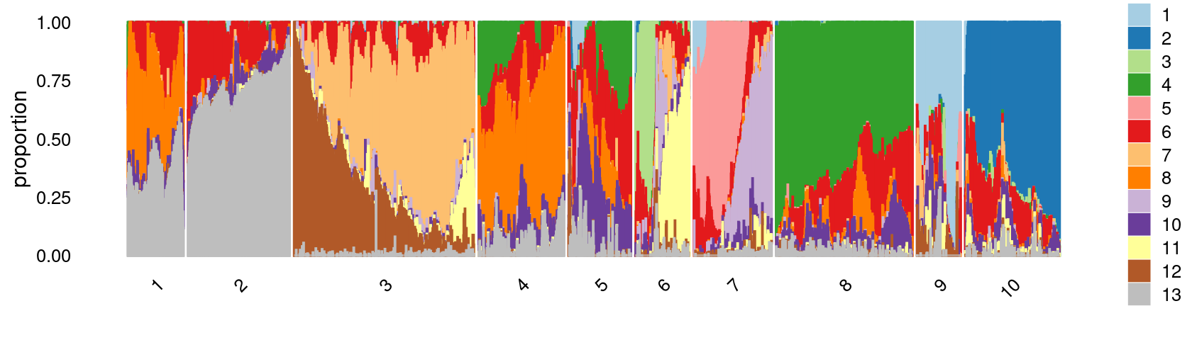
| Version | Author | Date |
|---|---|---|
| 697d54e | kevinlkx | 2020-10-21 |
Define clusters using k-means with \(k = 12\):
set.seed(10)

clusters.12 <- factor(kmeans(poisson2multinom(fit)$L,centers = 12)$cluster)
print(sort(table(clusters.12),decreasing = TRUE))
# clusters.12
#     3     8     2    10     4     5    12     1    11     6     7     9
# 15412  8326  8133  8036  7826  6055  5953  4474  4044  3584  2577  1548
Structure plot based on k-means clusters
colors_topics <- c("#a6cee3","#1f78b4","#b2df8a","#33a02c","#fb9a99","#e31a1c",
                   "#fdbf6f","#ff7f00","#cab2d6","#6a3d9a","#ffff99","#b15928",
                   "gray")
rows <- sample(nrow(fit$L),4000)

p.structure.3 <- structure_plot(select(poisson2multinom(fit),loadings = rows),
                     grouping = clusters.12[rows],n = Inf,gap = 20,
                     perplexity = 50,topics = 1:13,colors = colors_topics,
                     num_threads = 4,verbose = FALSE)
# Perplexity automatically changed to 47 because original setting of 50 was too large for the number of samples (145)
# Perplexity automatically changed to 25 because original setting of 50 was too large for the number of samples (79)
print(p.structure.3)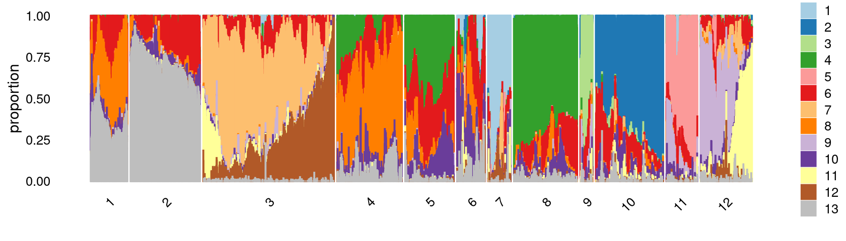
| Version | Author | Date |
|---|---|---|
| 697d54e | kevinlkx | 2020-10-21 |
Refine clusters
We then further refine the clusters based on k-means result with \(k = 12\): merge clusters 5 and 8.
clusters.merged <- clusters.12
clusters.merged[clusters.12 %in% c(5,8)] <- 5
clusters.merged <- factor(clusters.merged, labels = paste0("c", c(1:length(unique(clusters.merged)))))
print(sort(table(clusters.merged),decreasing = TRUE))

samples$cluster_kmeans <- clusters.merged
# clusters.merged
#    c3    c5    c2    c9    c4   c11    c1   c10    c6    c7    c8
# 15412 14381  8133  8036  7826  5953  4474  4044  3584  2577  1548
colors_topics <- c("#a6cee3","#1f78b4","#b2df8a","#33a02c","#fb9a99","#e31a1c",
"#fdbf6f","#ff7f00","#cab2d6","#6a3d9a","#ffff99","#b15928",
"gray")
rows <- sample(nrow(fit$L),4000)
p.structure.refined <- structure_plot(select(poisson2multinom(fit),loadings = rows),
grouping = clusters.merged[rows],n = Inf,gap = 20,
perplexity = 50,topics = 1:13,colors = colors_topics,
num_threads = 4,verbose = FALSE)
# Perplexity automatically changed to 42 because original setting of 50 was too large for the number of samples (130)
# Perplexity automatically changed to 26 because original setting of 50 was too large for the number of samples (82)
print(p.structure.refined)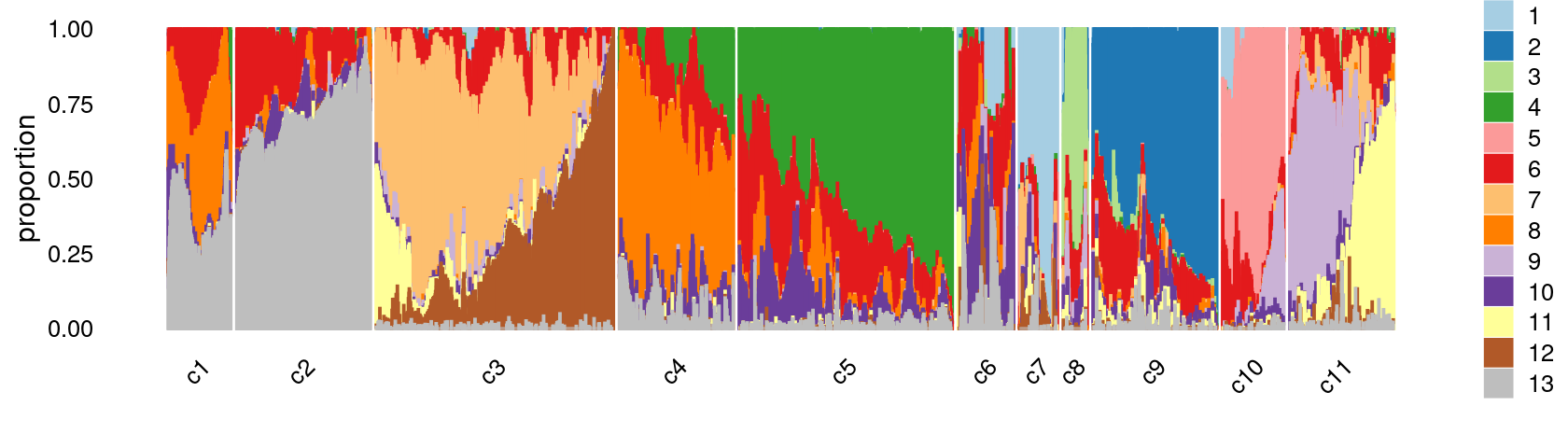
| Version | Author | Date |
|---|---|---|
| 697d54e | kevinlkx | 2020-10-21 |
The clusters defined by k-means on topic proportions reasonably identify the clusters shown in the PCA hexbin plots (below).
p.pca.4.1 <- labeled_pca_plot(fit,1:2,samples$cluster_kmeans,font_size = 7,
                       legend_label = "cluster_kmeans")
p.pca.4.2 <- labeled_pca_plot(fit,3:4,samples$cluster_kmeans,font_size = 7,
                       legend_label = "cluster_kmeans")
p.pca.4.3 <- labeled_pca_plot(fit,5:6,samples$cluster_kmeans,font_size = 7,
                       legend_label = "cluster_kmeans")
p.pca.4.4 <- labeled_pca_plot(fit,7:8,samples$cluster_kmeans,font_size = 7,
                       legend_label = "cluster_kmeans")
p.pca.4.5 <- labeled_pca_plot(fit,9:10,samples$cluster_kmeans,font_size = 7,
                       legend_label = "cluster_kmeans")
p.pca.4.6 <- labeled_pca_plot(fit,11:12,samples$cluster_kmeans,font_size = 7,
                       legend_label = "cluster_kmeans")
plot_grid(p.pca.4.1,p.pca.4.2,p.pca.4.3,p.pca.4.4,p.pca.4.5,p.pca.4.6)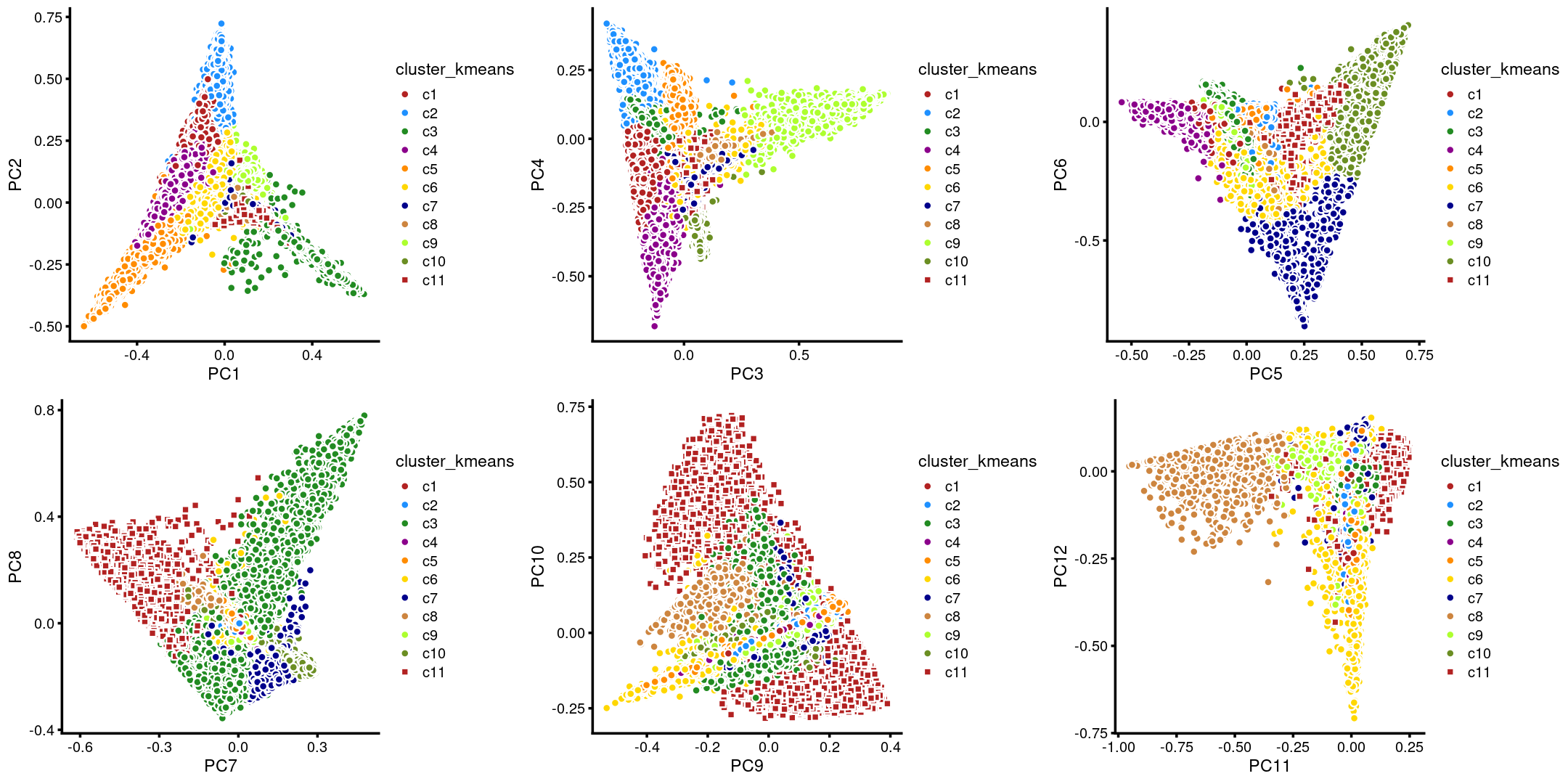
| Version | Author | Date |
|---|---|---|
| 697d54e | kevinlkx | 2020-10-21 |
plot_grid(p.pca2.1,p.pca2.2,p.pca2.3,p.pca2.4,p.pca2.5,p.pca2.6)
| Version | Author | Date |
|---|---|---|
| 697d54e | kevinlkx | 2020-10-21 |
We then label the cells in each cluster with the known cell labels.
Cell labels:
samples$Cluster <- as.factor(samples$Cluster)
cat(length(levels(samples$Cluster)), "cell labels. \n")
table(samples$Cluster)
# 15 cell labels.
#
#         B       CD4       CD8       CLP Collision Ery-early  Ery-late      HSPC
#      3731     18042      9304       216      3235      2453      1095      3033
#  HSPC-ery    Mono-1    Mono-2        NK       pDC      preB      proB
#      1774     10020      6687      8386       936      5954      1102
Plot the distribution of cell labels by clusters.
Stacked barplot for the counts of cell labels by clusters:
library(plyr);library(dplyr)
library(RColorBrewer)

freq_cluster_tissue <- count(samples, vars=c("cluster_kmeans","Cluster"))
n_colors <- length(levels(samples$Cluster))
colors_labels <- colorRampPalette(brewer.pal(9, "Set1"))(n_colors)

# stacked barplot for the counts of cell labels by clusters
p.barplot.1 <- ggplot(freq_cluster_tissue, aes(fill=Cluster, y=freq, x=cluster_kmeans)) +
  geom_bar(position="stack", stat="identity") +
  theme_classic() + xlab("Cluster") + ylab("Number of cells") +
  scale_fill_manual(values = colors_labels) +
  guides(fill=guide_legend(ncol=2)) +
  theme(
  legend.title = element_text(size = 10),
  legend.text = element_text(size = 8)
  )
print(p.barplot.1)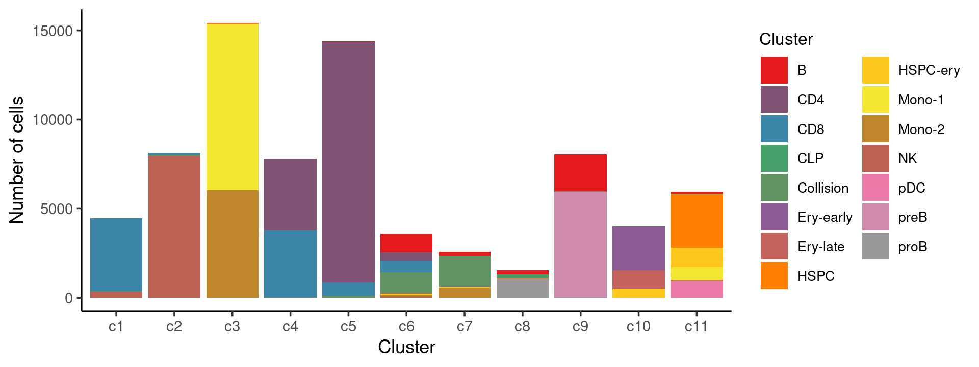
| Version | Author | Date |
|---|---|---|
| 697d54e | kevinlkx | 2020-10-21 |
Percent stacked barplot for the counts of cell labels by clusters:
freq_cluster_tissue <- count(samples, vars=c("cluster_kmeans","Cluster"))
n_colors <- length(levels(samples$Cluster))
colors_labels <- colorRampPalette(brewer.pal(9, "Set1"))(n_colors)

p.barplot.2 <- ggplot(freq_cluster_tissue, aes(fill=Cluster, y=freq, x=cluster_kmeans)) +
  geom_bar(position="fill", stat="identity") +
  theme_classic() + xlab("Cluster") + ylab("Proportion of cells") +
  scale_fill_manual(values = colors_labels) +
  guides(fill=guide_legend(ncol=2)) +
  theme(
  legend.title = element_text(size = 10),
  legend.text = element_text(size = 8)
  )
print(p.barplot.2)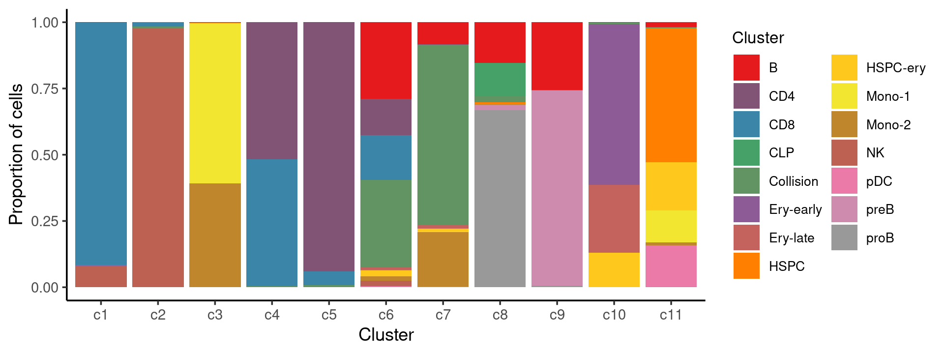
| Version | Author | Date |
|---|---|---|
| 697d54e | kevinlkx | 2020-10-21 |
We can see a few clusters are dominated by one major cell type: * cells in cluster c1 are primarily CD8 cells; * cells in cluster c2 are primarily NK cells; * cells in cluster c5 are primarily CD4 cells.
Some clusters are combinations of related cell types: * cells in cluster c3 are a combination of Mono-1 and Mono-2 cells; * cells in cluster c4 are a combination of CD4 and CD8 cells; * cells in cluster c9 are a combination of B and preB cells; * cells in cluster c10 are a combination of Ery-early, Ery-late and HSPC-ery cells;
Clusters c6, c7, c8, c11 are more heterogeneous with multiple cell types.
freq_cluster_cells <- with(samples,table(Cluster,cluster_kmeans))
print(freq_cluster_cells)
#            cluster_kmeans
# Cluster        c1    c2    c3    c4    c5    c6    c7    c8    c9   c10   c11
#   B             5     4    33     3    28  1033   216   238  2060     3   108
#   CD4           4     0     0  4046 13495   494     1     0     0     0     2
#   CD8        4086   127     1  3739   742   608     1     0     0     0     0
#   CLP           0     0     0     0     0     0     0   195     0     0    21
#   Collision    16    55     0    36   111  1182  1757    35    11    29     3
#   Ery-early     1     0     0     0     0     0     0     0     0  2452     0
#   Ery-late      0     0     0     0     0    31    34     0     0  1030     0
#   HSPC          0     1     5     0     0     7     0    11     0     0  3009
#   HSPC-ery      0     1    53     0     3    81    26     1     0   529  1080
#   Mono-1        0     0  9287     0     0     1     6     0     0     0   726
#   Mono-2        1     1  6032     0     2    57   529     1     0     0    64
#   NK          361  7944     0     2     0    77     1     0     0     1     0
#   pDC           0     0     0     0     0     8     4     0     0     0   924
#   preB          0     0     0     0     0     5     0    32  5917     0     0
#   proB          0     0     1     0     0     0     2  1035    48     0    16
sessionInfo()
# R version 3.5.1 (2018-07-02)
# Platform: x86_64-pc-linux-gnu (64-bit)
# Running under: Scientific Linux 7.4 (Nitrogen)
#
# Matrix products: default
# BLAS/LAPACK: /software/openblas-0.2.19-el7-x86_64/lib/libopenblas_haswellp-r0.2.19.so
#
# locale:
#  [1] LC_CTYPE=en_US.UTF-8       LC_NUMERIC=C
#  [3] LC_TIME=en_US.UTF-8        LC_COLLATE=en_US.UTF-8
#  [5] LC_MONETARY=en_US.UTF-8    LC_MESSAGES=en_US.UTF-8
#  [7] LC_PAPER=en_US.UTF-8       LC_NAME=C
#  [9] LC_ADDRESS=C               LC_TELEPHONE=C
# [11] LC_MEASUREMENT=en_US.UTF-8 LC_IDENTIFICATION=C
#
# attached base packages:
# [1] stats     graphics  grDevices utils     datasets  methods   base
#
# other attached packages:
# [1] RColorBrewer_1.1-2 plyr_1.8.6         fastTopics_0.3-180 cowplot_1.0.0
# [5] ggplot2_3.3.0      dplyr_0.8.5        Matrix_1.2-15      workflowr_1.6.2
#
# loaded via a namespace (and not attached):
#  [1] ggrepel_0.8.2      Rcpp_1.0.4.6       lattice_0.20-38    tidyr_0.8.3
#  [5] prettyunits_1.1.1  assertthat_0.2.1   rprojroot_1.3-2    digest_0.6.25
#  [9] R6_2.4.1           backports_1.1.7    MatrixModels_0.4-1 evaluate_0.14
# [13] coda_0.19-2        httr_1.4.1         pillar_1.4.4       rlang_0.4.6
# [17] progress_1.2.2     lazyeval_0.2.2     data.table_1.12.8  irlba_2.3.3
# [21] SparseM_1.77       whisker_0.4        hexbin_1.28.1      rmarkdown_2.1
# [25] labeling_0.3       Rtsne_0.15         stringr_1.4.0      htmlwidgets_1.5.1
# [29] munsell_0.5.0      compiler_3.5.1     httpuv_1.5.3.1     xfun_0.14
# [33] pkgconfig_2.0.3    mcmc_0.9-7         htmltools_0.4.0    tidyselect_0.2.5
# [37] tibble_3.0.1       quadprog_1.5-5     viridisLite_0.3.0  crayon_1.3.4
# [41] withr_2.1.2        later_1.0.0        MASS_7.3-51.6      grid_3.5.1
# [45] jsonlite_1.6       gtable_0.3.0       lifecycle_0.2.0    git2r_0.27.1
# [49] magrittr_1.5       scales_1.1.1       RcppParallel_4.4.3 stringi_1.4.6
# [53] farver_2.0.3       fs_1.3.1           promises_1.1.0     ellipsis_0.3.1
# [57] vctrs_0.3.0        tools_3.5.1        glue_1.4.1         purrr_0.3.4
# [61] hms_0.4.2          yaml_2.2.0         colorspace_1.4-1   plotly_4.8.0
# [65] knitr_1.28         quantreg_5.36      MCMCpack_1.4-4