Enhanced Visualization and Exploration of Pancreas Data using Seurat
Sagnik Nandy
Last updated: 2024-11-09
Checks: 7 0
Knit directory:
single-cell-jamboree/analysis/
This reproducible R Markdown analysis was created with workflowr (version 1.7.1). The Checks tab describes the reproducibility checks that were applied when the results were created. The Past versions tab lists the development history.
Great! Since the R Markdown file has been committed to the Git repository, you know the exact version of the code that produced these results.
Great job! The global environment was empty. Objects defined in the global environment can affect the analysis in your R Markdown file in unknown ways. For reproduciblity it’s best to always run the code in an empty environment.
The command set.seed(1) was run prior to running the
code in the R Markdown file. Setting a seed ensures that any results
that rely on randomness, e.g. subsampling or permutations, are
reproducible.
Great job! Recording the operating system, R version, and package versions is critical for reproducibility.
Nice! There were no cached chunks for this analysis, so you can be confident that you successfully produced the results during this run.
Great job! Using relative paths to the files within your workflowr project makes it easier to run your code on other machines.
Great! You are using Git for version control. Tracking code development and connecting the code version to the results is critical for reproducibility.
The results in this page were generated with repository version 47ab928. See the Past versions tab to see a history of the changes made to the R Markdown and HTML files.
Note that you need to be careful to ensure that all relevant files for
the analysis have been committed to Git prior to generating the results
(you can use wflow_publish or
wflow_git_commit). workflowr only checks the R Markdown
file, but you know if there are other scripts or data files that it
depends on. Below is the status of the Git repository when the results
were generated:
Untracked files:
    Untracked:  analysis/combined_umap_plot.png
    Untracked:  data/pancreas.RData
    Untracked:  scripts/Customized_Plots.R
Note that any generated files, e.g. HTML, png, CSS, etc., are not included in this status report because it is ok for generated content to have uncommitted changes.
These are the previous versions of the repository in which changes were
made to the R Markdown
(analysis/Exploration_pancreas_data_using_Seurat.Rmd) and
HTML (docs/Exploration_pancreas_data_using_Seurat.html)
files. If you’ve configured a remote Git repository (see
?wflow_git_remote), click on the hyperlinks in the table
below to view the files as they were in that past version.
| File | Version | Author | Date | Message |
|---|---|---|---|---|
| Rmd | 47ab928 | Sagnik-Nandy | 2024-11-09 | wflow_publish("analysis/Exploration_pancreas_data_using_Seurat.Rmd") |
| Rmd | 91670e5 | Peter Carbonetto | 2024-11-06 | A few minor fixes to Sagnik’s rmd. |
| Rmd | d9bb7a3 | GitHub | 2024-11-05 | Update Exploration_pancreas_data_using_Seurat.Rmd |
| html | 782250e | Sagnik-Nandy | 2024-11-04 | Build site. |
| html | d3c89dc | Sagnik-Nandy | 2024-11-04 | Initial commit |
| Rmd | a93bfc2 | GitHub | 2024-11-04 | Update Exploration_pancreas_data_using_Seurat.Rmd |
| Rmd | af5196f | GitHub | 2024-11-04 | Update Exploration_pancreas_data_using_Seurat.Rmd |
| Rmd | 95b96c1 | GitHub | 2024-11-04 | Update and rename Exploration_pancreas_data_using_Seurat to Exploration_pancreas_data_using_Seurat.Rmd |
In this analysis, we aim to generate an improved visualization of
pancreas data from the 2022 benchmarking study by Luecken et al.
using the Seurat package in R. This analysis uses the pre-processed
dataset, pancreas.RData.
1. Load Libraries
Load the necessary libraries for data analysis, plotting, and Seurat analysis.
library(Seurat)
library(tidyverse)
library(patchwork)
library(cowplot)
library(RColorBrewer)
library(Biobase)
library(clusterSim)
library(fpc)
library(ggpubr)
library(gridExtra)
2. Define Custom Functions
Define any custom functions for the analysis. This includes a
customized plotting function for dimensional reduction (e.g., UMAP or
PCA) and a function to create an elbow plot of the top variable features
in a Seurat object. I have already defined them and stored them in
Scripts folder with the name
Customized_Plots.R.
source("../Scripts/Customized_Plots.R")3. Set Working Directory and Load Data
Load the dataset, which contains “counts” and “sample_info”.
# Load the pancreas data from the data directory
load("../data/pancreas.RData")
4. Study Size Factors
Visualize the distribution of total counts (size factors) per cell in log scale.
s <- rowSums(counts)
pdat <- data.frame(log_size_factor = log10(s))
ggplot(pdat, aes(log_size_factor)) +
  geom_histogram(bins = 64, col = "black", fill = "black") +
  labs(x = "Log(Size Factor)") +
  theme_cowplot(font_size = 10)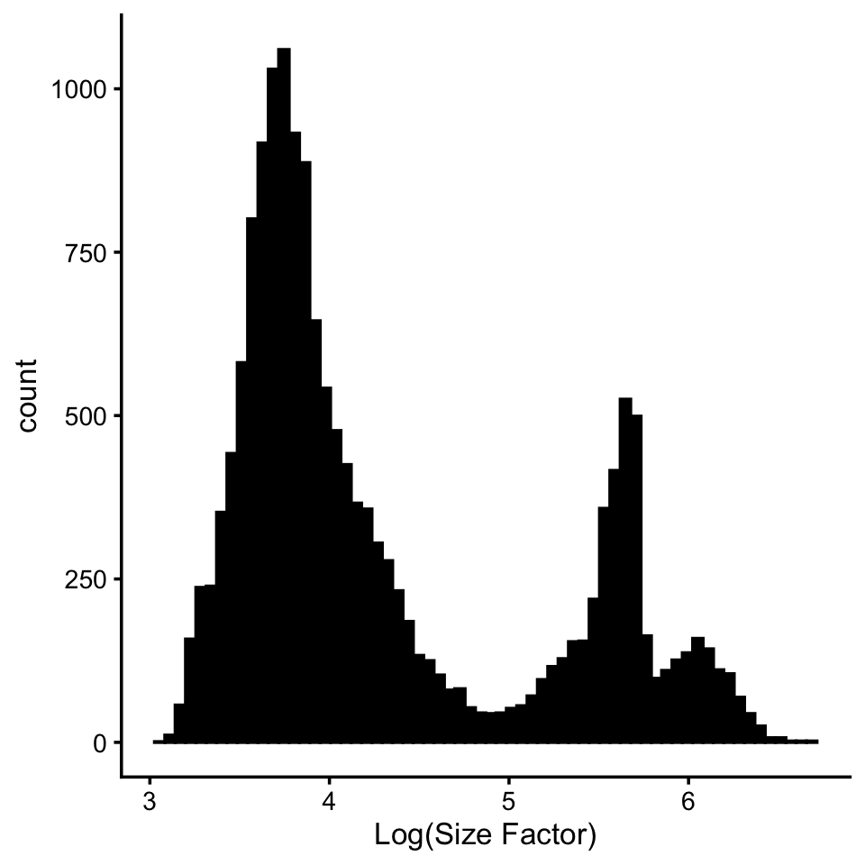
| Version | Author | Date |
|---|---|---|
| d3c89dc | Sagnik-Nandy | 2024-11-04 |
5. Study Gene Expression Levels
Examine the distribution of gene expression levels in the dataset.
p <- counts[counts > 0]  # Filter non-zero counts
pdat <- data.frame(log_rel_expression_level = log10(p))
ggplot(pdat, aes(log_rel_expression_level)) +
  geom_histogram(bins = 64, col = "black", fill = "black") +
  labs(x = "Log-Expression Level (Relative)") +
  theme_cowplot(font_size = 10)
| Version | Author | Date |
|---|---|---|
| d3c89dc | Sagnik-Nandy | 2024-11-04 |
6. Create Seurat Object
Create a Seurat object from the counts data, using
sample_info as metadata. Normalize the data with a custom
scale factor based on the mean size factor.
pancreas <- CreateSeuratObject(counts = t(counts), project = "pancreas", meta.data = sample_info)
scale_factor <- mean(s)
pancreas <- NormalizeData(pancreas, normalization.method = "LogNormalize", scale.factor = scale_factor)
7. Identify Variable Features
Identify the top 5,000 variable genes.
pancreas <- FindVariableFeatures(pancreas, selection.method = "vst", nfeatures = 5000)
VariableFeaturePlot(pancreas)
# Warning in scale_x_log10(): log-10 transformation introduced infinite values.
| Version | Author | Date |
|---|---|---|
| d3c89dc | Sagnik-Nandy | 2024-11-04 |
8. Elbow Plot of Variable Features
Generate an elbow plot to analyze variance across the top variable features.
create_elbow_plot(object = pancreas, assay = "RNA", k = 5000)
| Version | Author | Date |
|---|---|---|
| d3c89dc | Sagnik-Nandy | 2024-11-04 |
9. Select Top 1,000 Variable Features
Select the top 1,000 variable genes for further analysis.
desired_genes <- head(VariableFeatures(pancreas), 1000)10. Scale Data and Run PCA
Scale the data for the selected features and run PCA.
pancreas <- ScaleData(pancreas, features = desired_genes)
pancreas <- RunPCA(pancreas, assay = "RNA", features = desired_genes)
ElbowPlot(pancreas, ndims = 50)
| Version | Author | Date |
|---|---|---|
| d3c89dc | Sagnik-Nandy | 2024-11-04 |
11. Run UMAP
Perform UMAP using the top 25 principal components.
pancreas <- RunUMAP(pancreas, dims = 1:25)
# Warning: The default method for RunUMAP has changed from calling Python UMAP via reticulate to the R-native UWOT using the cosine metric
# To use Python UMAP via reticulate, set umap.method to 'umap-learn' and metric to 'correlation'
# This message will be shown once per session
umap_embeddings <- Embeddings(object = pancreas, reduction = "umap")
12. Define Colors for Cell Types
Define a color vector for distinguishing 14 different cell types.
col_vector <- c(
  "#E41A1C", "#377EB8", "#4DAF4A", "#984EA3", "#FF7F00",
  "#FFFF33", "#A65628", "#999999", "#66C2A5", "#FC8D62",
  "#8DA0CB", "#E78AC3", "#A6D854", "#FFD92F"
)
13. Create UMAP Plots by Cell Type and Technology
Generate UMAP plots where cell types are represented by colors and technology by shapes.
# Create UMAP Plots by Cell Type and Technology
p1 <- DimPlotSagnik(umap_embeddings, group.by = sample_info$celltype, pt.size = 0.04, cols = col_vector) +
  theme(plot.title = element_text(hjust = 0.5)) +
  ggtitle("UMAP of Pancreas Cells by Cell Type")
p2 <- DimPlotSagnik(umap_embeddings, group.by = sample_info$tech, pt.size = 0.04, cols = col_vector) +
  theme(plot.title = element_text(hjust = 0.5)) +
  ggtitle("UMAP of Pancreas Cells by Technology")

# Combine plots side-by-side
combined_plot <- p1 + p2 + plot_layout(ncol = 2)
combined_plot
| Version | Author | Date |
|---|---|---|
| d3c89dc | Sagnik-Nandy | 2024-11-04 |
ggsave(
  filename = "combined_umap_plot.png",    # File name and format
  plot = combined_plot,                   # The plot object to save
  width = 15,                             # Width in inches
  height = 6,                             # Height in inches
  dpi = 300                               # Resolution in dots per inch (for high-quality output)
)
sessionInfo()
# R version 4.4.1 (2024-06-14)
# Platform: aarch64-apple-darwin20
# Running under: macOS 15.0.1
#
# Matrix products: default
# BLAS:   /Library/Frameworks/R.framework/Versions/4.4-arm64/Resources/lib/libRblas.0.dylib
# LAPACK: /Library/Frameworks/R.framework/Versions/4.4-arm64/Resources/lib/libRlapack.dylib;  LAPACK version 3.12.0
#
# locale:
# [1] en_US.UTF-8/en_US.UTF-8/en_US.UTF-8/C/en_US.UTF-8/en_US.UTF-8
#
# time zone: America/Chicago
# tzcode source: internal
#
# attached base packages:
# [1] stats     graphics  grDevices utils     datasets  methods   base
#
# other attached packages:
#  [1] gridExtra_2.3       ggpubr_0.6.0        fpc_2.2-13
#  [4] clusterSim_0.51-5   MASS_7.3-61         cluster_2.1.6
#  [7] Biobase_2.64.0      BiocGenerics_0.50.0 RColorBrewer_1.1-3
# [10] cowplot_1.1.3       patchwork_1.3.0     lubridate_1.9.3
# [13] forcats_1.0.0       stringr_1.5.1       dplyr_1.1.4
# [16] purrr_1.0.2         readr_2.1.5         tidyr_1.3.1
# [19] tibble_3.2.1        ggplot2_3.5.1       tidyverse_2.0.0
# [22] Seurat_5.1.0        SeuratObject_5.0.2  sp_2.1-4
#
# loaded via a namespace (and not attached):
#   [1] RcppAnnoy_0.0.22       splines_4.4.1          later_1.3.2
#   [4] polyclip_1.10-7        fastDummies_1.7.4      lifecycle_1.0.4
#   [7] rstatix_0.7.2          rprojroot_2.0.4        globals_0.16.3
#  [10] lattice_0.22-6         prabclus_2.3-4         backports_1.5.0
#  [13] magrittr_2.0.3         plotly_4.10.4          sass_0.4.9
#  [16] rmarkdown_2.28         jquerylib_0.1.4        yaml_2.3.10
#  [19] httpuv_1.6.15          sctransform_0.4.1      spam_2.11-0
#  [22] flexmix_2.3-19         spatstat.sparse_3.1-0  reticulate_1.39.0
#  [25] pbapply_1.7-2          ade4_1.7-22            abind_1.4-8
#  [28] Rtsne_0.17             nnet_7.3-19            git2r_0.35.0
#  [31] ggrepel_0.9.6          irlba_2.3.5.1          listenv_0.9.1
#  [34] spatstat.utils_3.1-0   goftest_1.2-3          RSpectra_0.16-2
#  [37] spatstat.random_3.3-2  fitdistrplus_1.2-1     parallelly_1.38.0
#  [40] leiden_0.4.3.1         codetools_0.2-20       tidyselect_1.2.1
#  [43] farver_2.1.2           matrixStats_1.4.1      stats4_4.4.1
#  [46] spatstat.explore_3.3-3 jsonlite_1.8.9         e1071_1.7-16
#  [49] progressr_0.15.0       Formula_1.2-5          ggridges_0.5.6
#  [52] survival_3.7-0         systemfonts_1.1.0      tools_4.4.1
#  [55] ragg_1.3.3             ica_1.0-3              Rcpp_1.0.13
#  [58] glue_1.8.0             xfun_0.48              withr_3.0.2
#  [61] fastmap_1.2.0          fansi_1.0.6            digest_0.6.37
#  [64] timechange_0.3.0       R6_2.5.1               mime_0.12
#  [67] textshaping_0.4.0      colorspace_2.1-1       scattermore_1.2
#  [70] tensor_1.5             spatstat.data_3.1-2    diptest_0.77-1
#  [73] utf8_1.2.4             generics_0.1.3         data.table_1.16.2
#  [76] robustbase_0.99-4-1    class_7.3-22           httr_1.4.7
#  [79] htmlwidgets_1.6.4      whisker_0.4.1          uwot_0.2.2
#  [82] pkgconfig_2.0.3        gtable_0.3.6           modeltools_0.2-23
#  [85] workflowr_1.7.1        lmtest_0.9-40          htmltools_0.5.8.1
#  [88] carData_3.0-5          dotCall64_1.2          scales_1.3.0
#  [91] png_0.1-8              spatstat.univar_3.0-1  knitr_1.48
#  [94] rstudioapi_0.17.1      tzdb_0.4.0             reshape2_1.4.4
#  [97] nlme_3.1-166           proxy_0.4-27           cachem_1.1.0
# [100] zoo_1.8-12             KernSmooth_2.23-24     parallel_4.4.1
# [103] miniUI_0.1.1.1         pillar_1.9.0           grid_4.4.1
# [106] vctrs_0.6.5            RANN_2.6.2             promises_1.3.0
# [109] car_3.1-3              xtable_1.8-4           evaluate_1.0.1
# [112] cli_3.6.3              compiler_4.4.1         rlang_1.1.4
# [115] future.apply_1.11.3    ggsignif_0.6.4         labeling_0.4.3
# [118] mclust_6.1.1           plyr_1.8.9             fs_1.6.5
# [121] stringi_1.8.4          viridisLite_0.4.2      deldir_2.0-4
# [124] munsell_0.5.1          lazyeval_0.2.2         spatstat.geom_3.3-3
# [127] Matrix_1.7-1           RcppHNSW_0.6.0         hms_1.1.3
# [130] future_1.34.0          shiny_1.9.1            highr_0.11
# [133] kernlab_0.9-33         ROCR_1.0-11            igraph_2.1.1
# [136] broom_1.0.7            bslib_0.8.0            DEoptimR_1.1-3