A another look at matrix factorization for the pancreas data
Peter Carbonetto
Last updated: 2024-12-16
Checks: 6 1
Knit directory:
single-cell-jamboree/analysis/
This reproducible R Markdown analysis was created with workflowr (version 1.7.1). The Checks tab describes the reproducibility checks that were applied when the results were created. The Past versions tab lists the development history.
The R Markdown file has unstaged changes. To know which version of
the R Markdown file created these results, you’ll want to first commit
it to the Git repo. If you’re still working on the analysis, you can
ignore this warning. When you’re finished, you can run
wflow_publish to commit the R Markdown file and build the
HTML.
Great job! The global environment was empty. Objects defined in the global environment can affect the analysis in your R Markdown file in unknown ways. For reproduciblity it’s best to always run the code in an empty environment.
The command set.seed(1) was run prior to running the
code in the R Markdown file. Setting a seed ensures that any results
that rely on randomness, e.g. subsampling or permutations, are
reproducible.
Great job! Recording the operating system, R version, and package versions is critical for reproducibility.
Nice! There were no cached chunks for this analysis, so you can be confident that you successfully produced the results during this run.
Great job! Using relative paths to the files within your workflowr project makes it easier to run your code on other machines.
Great! You are using Git for version control. Tracking code development and connecting the code version to the results is critical for reproducibility.
The results in this page were generated with repository version 9b5463e. See the Past versions tab to see a history of the changes made to the R Markdown and HTML files.
Note that you need to be careful to ensure that all relevant files for
the analysis have been committed to Git prior to generating the results
(you can use wflow_publish or
wflow_git_commit). workflowr only checks the R Markdown
file, but you know if there are other scripts or data files that it
depends on. Below is the status of the Git repository when the results
were generated:
Ignored files:
    Ignored:    .Rhistory
    Ignored:    .Rproj.user/

Unstaged changes:
    Modified:   analysis/pancreas_another_look.Rmd
Note that any generated files, e.g. HTML, png, CSS, etc., are not included in this status report because it is ok for generated content to have uncommitted changes.
These are the previous versions of the repository in which changes were
made to the R Markdown (analysis/pancreas_another_look.Rmd)
and HTML (docs/pancreas_another_look.html) files. If you’ve
configured a remote Git repository (see ?wflow_git_remote),
click on the hyperlinks in the table below to view the files as they
were in that past version.
| File | Version | Author | Date | Message |
|---|---|---|---|---|
| Rmd | 9b5463e | WD | 2024-12-16 | adding NJ to additonal results |
| html | 9b5463e | WD | 2024-12-16 | adding NJ to additonal results |
| html | 1101c80 | Peter Carbonetto | 2024-12-16 | Added smartseq2 results to pancreas_another_look analysis. |
| Rmd | de661ca | Peter Carbonetto | 2024-12-16 | wflow_publish("pancreas_another_look.Rmd", verbose = TRUE) |
| Rmd | a2f2262 | Peter Carbonetto | 2024-12-16 | Added some results on the smartseq2 data to the ‘pancreas_another_look’ analysis. |
| Rmd | 9116341 | Peter Carbonetto | 2024-12-14 | Made a couple fixes to one of the structure plots in pancreas_another_look.Rmd. |
| html | 40e6f39 | Peter Carbonetto | 2024-12-14 | Added Structure plots to pancreas_another_look analysis for CEL-Seq2 data set. |
| Rmd | b6c1981 | Peter Carbonetto | 2024-12-14 | workflowr::wflow_publish("analysis/pancreas_another_look.Rmd", |
| Rmd | 3283b84 | Peter Carbonetto | 2024-12-13 | Added some structure plots to the pancreas_another_look analysis. |
| Rmd | e264e5b | Peter Carbonetto | 2024-12-12 | Created draft analysis in pancreas_celseq2.R; this will be incorporated into pancreas_another_look.Rmd. |
| html | c01f832 | Peter Carbonetto | 2024-12-12 | First build of the pancreas_another_look analysis. |
| Rmd | 04b172c | Peter Carbonetto | 2024-12-12 | workflowr::wflow_publish("pancreas_another_look.Rmd", view = FALSE) |
The previous analysis applied different matrix factorization approaches to the full pancreas data set. A key challenge in analyzing the full pancreas data set is that there are large batch or data-set effects, which some matrix factorization approaches have difficulty dealing with (particularly the topic model). Here we look more closely at a couple of the individual data sets to highlight better how the different factorizations yield different representations of the underlying structure in the cells without the added complication of dealing with the batch effects.
First, load the packages needed for this analysis.
library(Matrix)
library(fastTopics)
# Warning: package 'fastTopics' was built under R version 4.4.2
library(ggplot2)
library(cowplot)
library(ape)
# Warning: package 'ape' was built under R version 4.4.2
Set the seed for reproducibility.
set.seed(1)CEL-Seq2 data
Let’s start with the “CEL-Seq2” data from the Muraro et al 2016 paper. (The data were generated using the CEL-Seq2 protocol, hence the name.)
First load the CEL-Seq2 pancreas data and the outputs generated by
running the compute_pancreas_celseq2_factors.R script.
load("../data/pancreas.RData")
load("../output/pancreas_celseq2_factors.RData")
i           <- which(sample_info$tech == "celseq2")
sample_info <- sample_info[i,]
counts      <- counts[i,]
sample_info <- transform(sample_info,celltype = factor(celltype))
For fair comparison all the matrix factorizations were generated with 9 factors or topics.
Topic model (fastTopics)
Here is the topic model with 9 topics:
celltype <- sample_info$celltype
celltype <-
 factor(celltype,
        c("acinar","ductal","activated_stellate","quiescent_stellate",
          "endothelial","macrophage","mast","schwann","alpha","beta",
          "delta","gamma","epsilon"))
L <- poisson2multinom(pnmf)$L
structure_plot(L,grouping = celltype,gap = 20,perplexity = 70,n = Inf)
Most of the topics identify individual cell types or subsets of similar cell types. The topics also identify some substructures within and across cell types, e.g., topics 2 and 7. Most of the smaller cell types are not captured as a separate topic.
Lets just have a look at the distance between topic
dist_mat= t(pnmf$F)%*%pnmf$F
dimnames(dist_mat)= list(1:ncol(dist_mat), 1:ncol(dist_mat))
check_tree=nj(dist_mat )
plot(check_tree, main="TM +NJ")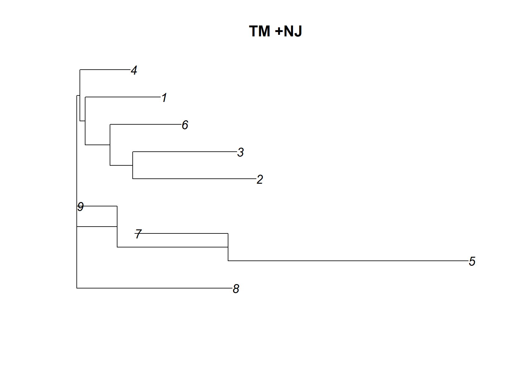
| Version | Author | Date |
|---|---|---|
| 9b5463e | WD | 2024-12-16 |
check_tree$edge.length=abs(check_tree$edge.length)
plot(check_tree)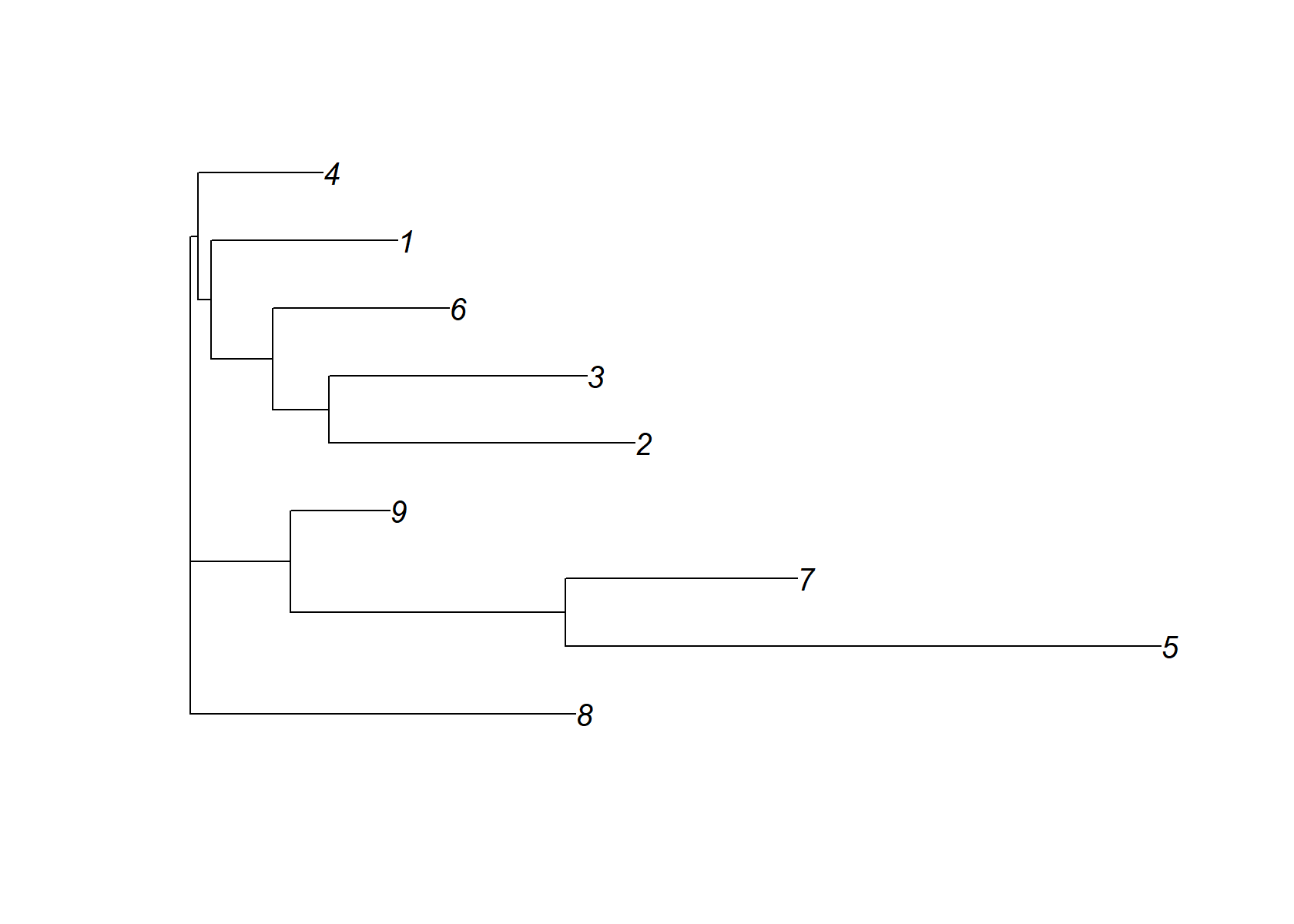
| Version | Author | Date |
|---|---|---|
| 9b5463e | WD | 2024-12-16 |
Flashier NMF
Let’s now compare the topic model to the empirical Bayes NMF result (with 9 factors).
I omit the first factor from the Structure plot because it is a “baseline” factor, and therefore not interesting to look at:
L <- fl_nmf_ldf$L
k <- ncol(L)
colnames(L) <- paste0("k",1:k)
structure_plot(L[,-1],grouping = celltype,gap = 20,perplexity = 70,n = Inf) +
  labs(y = "membership",fill = "factor",color = "factor")
It is interesting that the EBNMF factors distinguish some of the rare cell types, but do not distinguish as well among some of the islet cells (e.g., delta and gamma), even though they are quite abundant. It seems that these methods are each adept at identifying different types of structure.
dist_mat= t(fl_nmf_ldf$F[,-1])%*%fl_nmf_ldf$F[,-1]
dimnames(dist_mat)= list(2:ncol(fl_nmf_ldf$F), 2:ncol(fl_nmf_ldf$F))
check_tree=nj(dist_mat )
plot(check_tree, main="EBNMF +NJ")
| Version | Author | Date |
|---|---|---|
| 9b5463e | WD | 2024-12-16 |
check_tree$edge.length=abs(check_tree$edge.length)
plot(check_tree)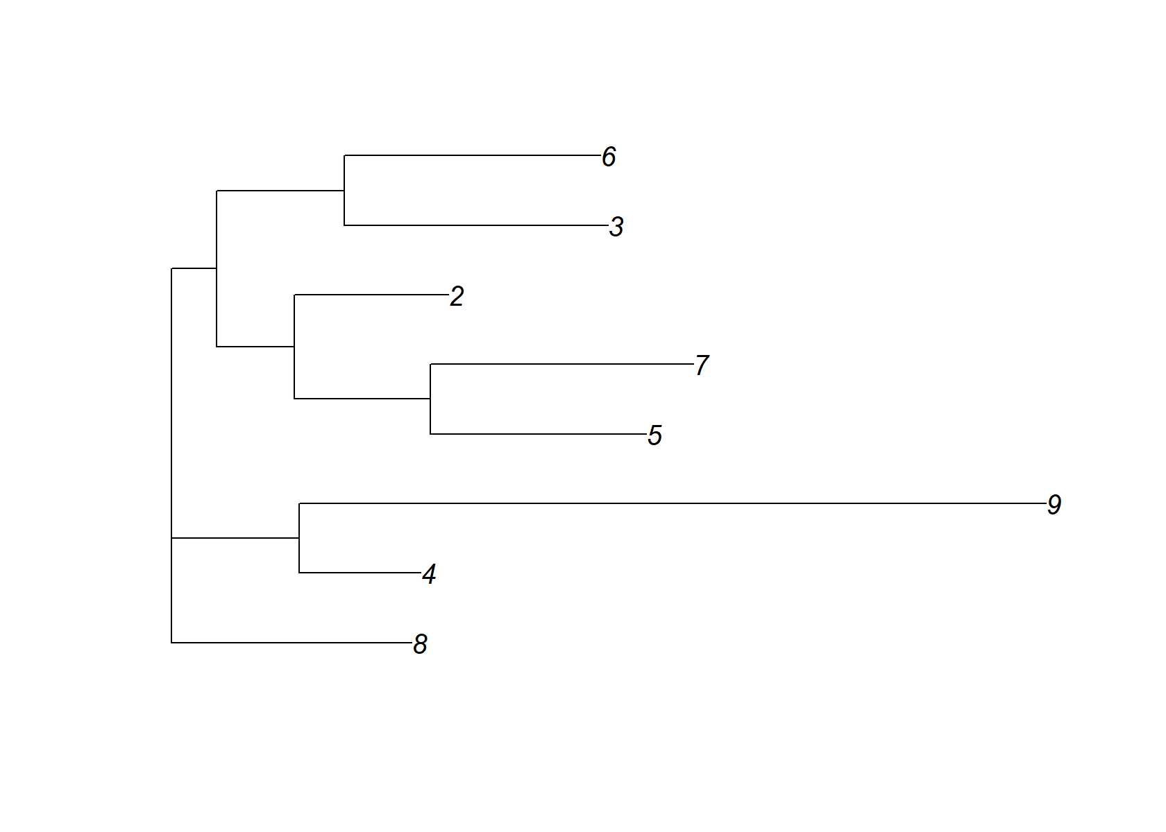
| Version | Author | Date |
|---|---|---|
| 9b5463e | WD | 2024-12-16 |
NMF (NNLM)
Let’s now have a look at the “vanilla” NMF (produced by the NNLM package). As before, this NMF has 9 factors.
scale_cols <- function (A, b)
  t(t(A) * b)
W <- nmf$W
k <- ncol(W)
d <- apply(W,2,max)
W <- scale_cols(W,1/d)
colnames(W) <- paste0("k",1:k)
structure_plot(W,grouping = celltype,gap = 20,perplexity = 70,n = Inf) +
  labs(y = "membership",fill = "factor",color = "factor")
Unlike the EBNMF results, there is no single factor that acts as a “baseline”. Some of the rarer cell types are missed by this NMF. It is also interesting that it has identified a single factor (k = 4) corresponding to all islet cells. Oddly, it seems to have identified factors that are active in the same cells, such as factors 3 and 6, as well as 7 and 8. So the NMF and EBNMF results are surprisingly different.
dist_mat=  (nmf$H )%*%t(nmf$H )
dimnames(dist_mat)= list(1:ncol(dist_mat), 1:ncol(dist_mat))
check_tree=nj(dist_mat )
plot(check_tree, main="NMF +NJ")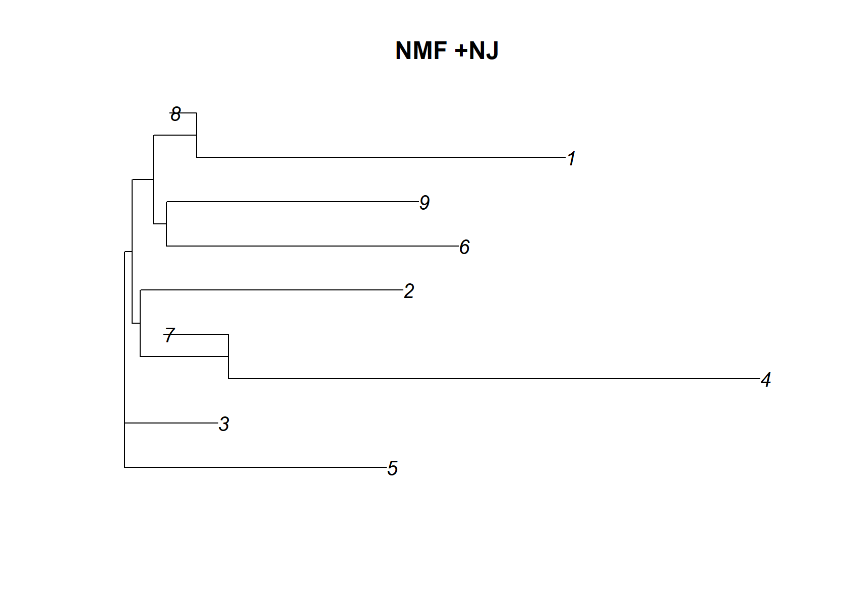
| Version | Author | Date |
|---|---|---|
| 9b5463e | WD | 2024-12-16 |
check_tree$edge.length=abs(check_tree$edge.length)
plot(check_tree)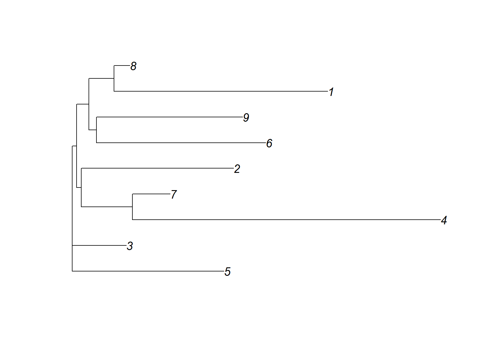
| Version | Author | Date |
|---|---|---|
| 9b5463e | WD | 2024-12-16 |
Flashier semi-NMF
The semi-NMF decomposition produced by flashier is interesting because it identifies not only cell-type-specific factors (e.g., factors 6, 7, 9), but also factors capturing expression programs common to several similar cell types (e.g., factors 2, 4, 8).
L <- fl_snmf_ldf$L
k <- ncol(L)
colnames(L) <- paste0("k",1:k)
structure_plot(L[,-c(1,5)],grouping = celltype,gap = 20,
               perplexity = 70,n = Inf) +
  labs(y = "membership",fill = "factor",color = "factor")
In other words, the semi-NMF is capturing structure at different levels of cell-type-specifity, achieving a cell-type “hierarchy” of sorts. Note that I removed two factors (1 and 5) from the Structure plot because they were active to varying degreees in all cells.
dist_mat= t(fl_snmf_ldf$F[,-c(1,5)] )%*%fl_snmf_ldf$F [,-c(1,5)]
dimnames(dist_mat)= list((1:ncol(fl_snmf_ldf$F))[-c(1,5)], (1:ncol(fl_snmf_ldf$F))[-c(1,5)])
check_tree=nj(dist_mat )
plot(check_tree, main="EBsNMF +NJ")
| Version | Author | Date |
|---|---|---|
| 9b5463e | WD | 2024-12-16 |
check_tree$edge.length=abs(check_tree$edge.length)
plot(check_tree)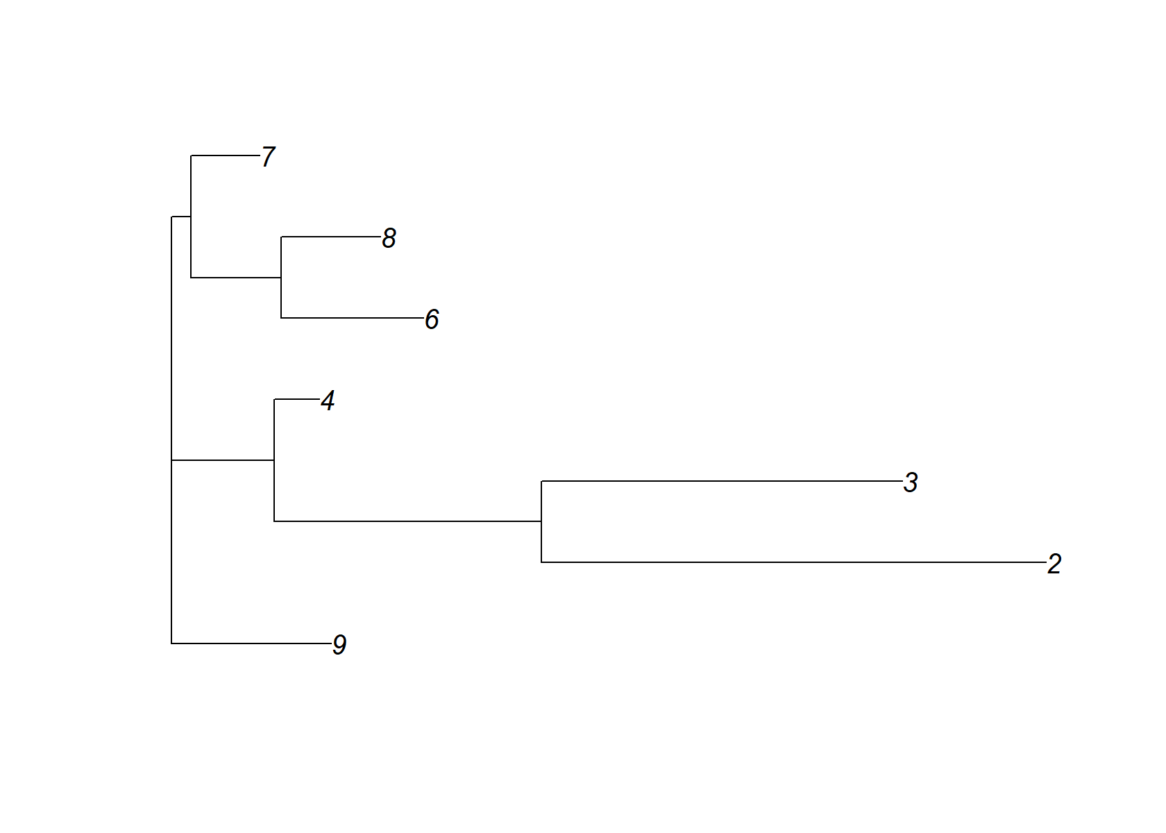
| Version | Author | Date |
|---|---|---|
| 9b5463e | WD | 2024-12-16 |
Smart-seq2 data
The “Smart-seq2” data from the Segerstolpe et al 2016 paper is another interesting pancreas data set that is roughly the same size as the CEL-Seq2 data set, and contains transcriptional profiles from some of the same cell types. (These data were generated using the “Smart-seq2” protocol, hence the name.) Let’s redo the comparisons above on this data set.
First load the Smart-Seq2 data and the outputs generated from running
the compute_pancreas_smartseq2_factors.R script.
load("../data/pancreas.RData")
load("../output/pancreas_smartseq2_factors.RData")
i           <- which(sample_info$tech == "smartseq2")
sample_info <- sample_info[i,]
counts      <- counts[i,]
sample_info <- transform(sample_info,celltype = factor(celltype))
celltype <- sample_info$celltype
celltype <-
 factor(celltype,
        c("acinar","ductal","activated_stellate","quiescent_stellate",
          "endothelial","macrophage","mast","schwann","alpha",
          "beta","delta","gamma","epsilon"))
Topic model (fastTopics)
Here is the topic model with 9 topics:
L <- poisson2multinom(pnmf)$L
structure_plot(L,grouping = celltype,gap = 20,perplexity = 70,n = Inf)
Broadly speaking, the topic model picks up very similar structure to the CEL-seq2 data. However, there are also some important differences. The most noticeable differences are that: (1) it does not identify a separate topic for ductal vs. stellate cells, etc; (2) there are at least two additional topics (topics 1 and 8) capturing additional variation across cell types that is not specific to cell type, and represents some additional variation in expression. It is possible that this additional variation in expression is due to differences in sex, age, BMI and/or disease status (T2D vs. healthy) among the 10 donors.
dist_mat= t(pnmf$F )%*%pnmf$F
dimnames(dist_mat)= list(1:ncol(dist_mat), 1:ncol(dist_mat))
check_tree=nj(dist_mat )
plot(check_tree, main="TM +NJ")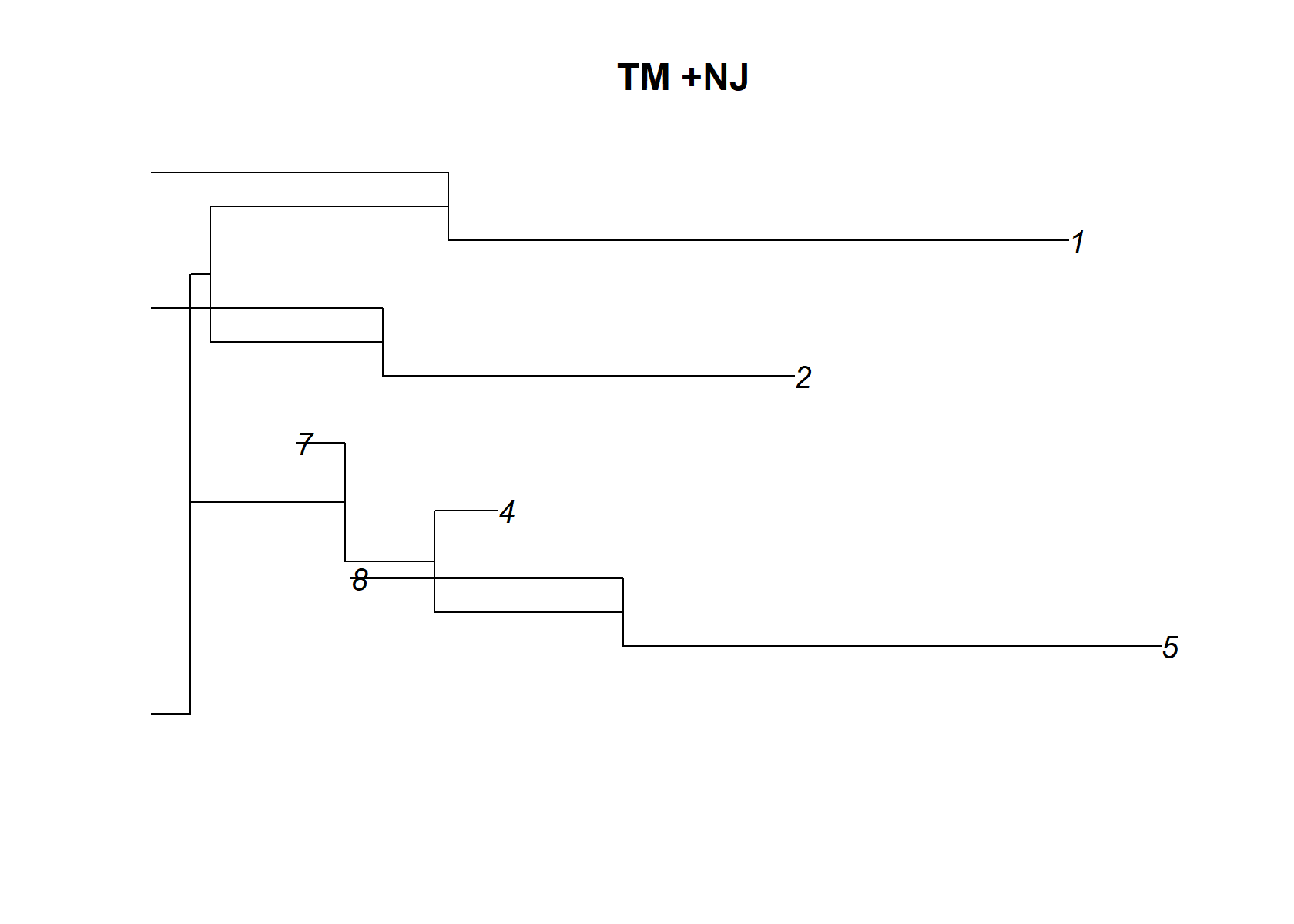
| Version | Author | Date |
|---|---|---|
| 9b5463e | WD | 2024-12-16 |
check_tree$edge.length=abs(check_tree$edge.length)
plot(check_tree)
| Version | Author | Date |
|---|---|---|
| 9b5463e | WD | 2024-12-16 |
Flashier NMF
Although the EBNMF result for the Smart-seq2 data set has some differences from the EBNMF result for the CEL-seq2 data set, there are some common trends: (1) it is better able to capture strucuture in the less abundance cell types (e.g., stellate cells); (2) the factors do not as clearly distinguish among the islet cells as the topics. Because there is other systematic variation in expression that is not cell-type-specific, this is picked up by several factors (factors 1, 8 and 9).
L <- fl_nmf_ldf$L
k <- ncol(L)
colnames(L) <- paste0("k",1:k)
celltype_topics  <- 2:7
other_topics <- c(1,8,9)
p1 <- structure_plot(L[,celltype_topics],grouping = celltype,gap = 20,
                     perplexity = 70,n = Inf) +
  labs(y = "membership",fill = "factor",color = "factor",
       title = "cell-type factors")
other_colors <- c("#66c2a5","#fc8d62","#8da0cb")
p2 <- structure_plot(L[,other_topics],grouping = celltype,gap = 20,
                     perplexity = 70,n = Inf) +
  labs(y = "membership",fill = "factor",color = "factor",
       title = "other factors") +
  scale_color_manual(values = other_colors) +
  scale_fill_manual(values = other_colors)
plot_grid(p1,p2,nrow = 2,ncol = 1)
dist_mat= t(fl_nmf_ldf$F[,celltype_topics])%*%fl_nmf_ldf$F[,celltype_topics]
dimnames(dist_mat)= list(2:7, 2:7)
check_tree=nj(dist_mat )
plot(check_tree, main="EBNMF +NJ")
| Version | Author | Date |
|---|---|---|
| 9b5463e | WD | 2024-12-16 |
check_tree$edge.length=abs(check_tree$edge.length)
plot(check_tree)
| Version | Author | Date |
|---|---|---|
| 9b5463e | WD | 2024-12-16 |
NMF (NNLM)
In the Smart-seq2 data set, the NMF decomposition generated by NNLM is remarkaby similar to the flashier NMF decomposition:
scale_cols <- function (A, b)
  t(t(A) * b)
W <- nmf$W
k <- ncol(W)
d <- apply(W,2,max)
W <- scale_cols(W,1/d)
colnames(W) <- paste0("k",1:k)
celltype_topics  <- c(3:6,8,9)
other_topics <- c(1,2,7)
p1 <- structure_plot(W[,celltype_topics],grouping = celltype,
                     gap = 20,perplexity = 70,n = Inf) +
  labs(y = "membership",fill = "factor",color = "factor",
       title = "cell-type factors")
p2 <- structure_plot(W[,other_topics],grouping = celltype,
                     gap = 20,perplexity = 70,n = Inf) +
  scale_color_manual(values = other_colors) +
  scale_fill_manual(values = other_colors) +
  labs(y = "membership",fill = "factor",color = "factor",
       title = "other factors")
plot_grid(p1,p2,nrow = 2,ncol = 1)
dist_mat=  (nmf$H[ celltype_topics,])%*%t(nmf$H[ celltype_topics,])
dimnames(dist_mat)= list(celltype_topics, celltype_topics)
check_tree=nj(dist_mat )
plot(check_tree, main="NMF +NJ")
| Version | Author | Date |
|---|---|---|
| 9b5463e | WD | 2024-12-16 |
check_tree$edge.length=abs(check_tree$edge.length)
plot(check_tree)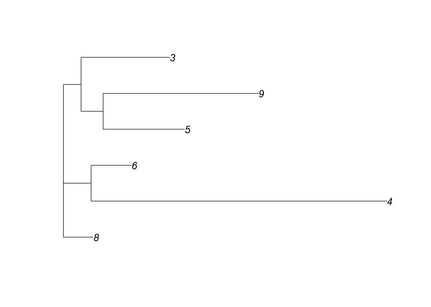
| Version | Author | Date |
|---|---|---|
| 9b5463e | WD | 2024-12-16 |
Flashier semi-NMF
The empirical Bayes semi-NMF decomposition is interesting in particular because it is capturing common expression patterns among some of the cell types (e.g., acinar, ductal, stellate) as well as their differences (e.g., separate factors for acinar, stellate, and quiescent stellate cells), and therefore the semi-NMF factors may represent particularly interpretable gene expression programs.
L <- fl_snmf_ldf$L
k <- ncol(L)
colnames(L) <- paste0("k",1:k)
celltype_topics  <- c(3,4,6,7,9)
other_topics <- c(1,5,8)
p1 <- structure_plot(L[,celltype_topics],grouping = celltype,
                     gap = 20,perplexity = 70,n = Inf) +
  labs(y = "membership",fill = "factor",color = "factor",
       title = "cell-type factors")
p2 <- structure_plot(L[,other_topics],grouping = celltype,
                     gap = 20,perplexity = 70,n = Inf) +
  scale_color_manual(values = other_colors) +
  scale_fill_manual(values = other_colors) +
  labs(y = "membership",fill = "factor",color = "factor",
       title = "other factors")
plot_grid(p1,p2,nrow = 2,ncol = 1)
dist_mat= t(fl_snmf_ldf$F[,celltype_topics])%*%fl_snmf_ldf$F[,celltype_topics]
dimnames(dist_mat)= list(celltype_topics,celltype_topics)
check_tree=nj(dist_mat )
plot(check_tree, main="sNMF +NJ")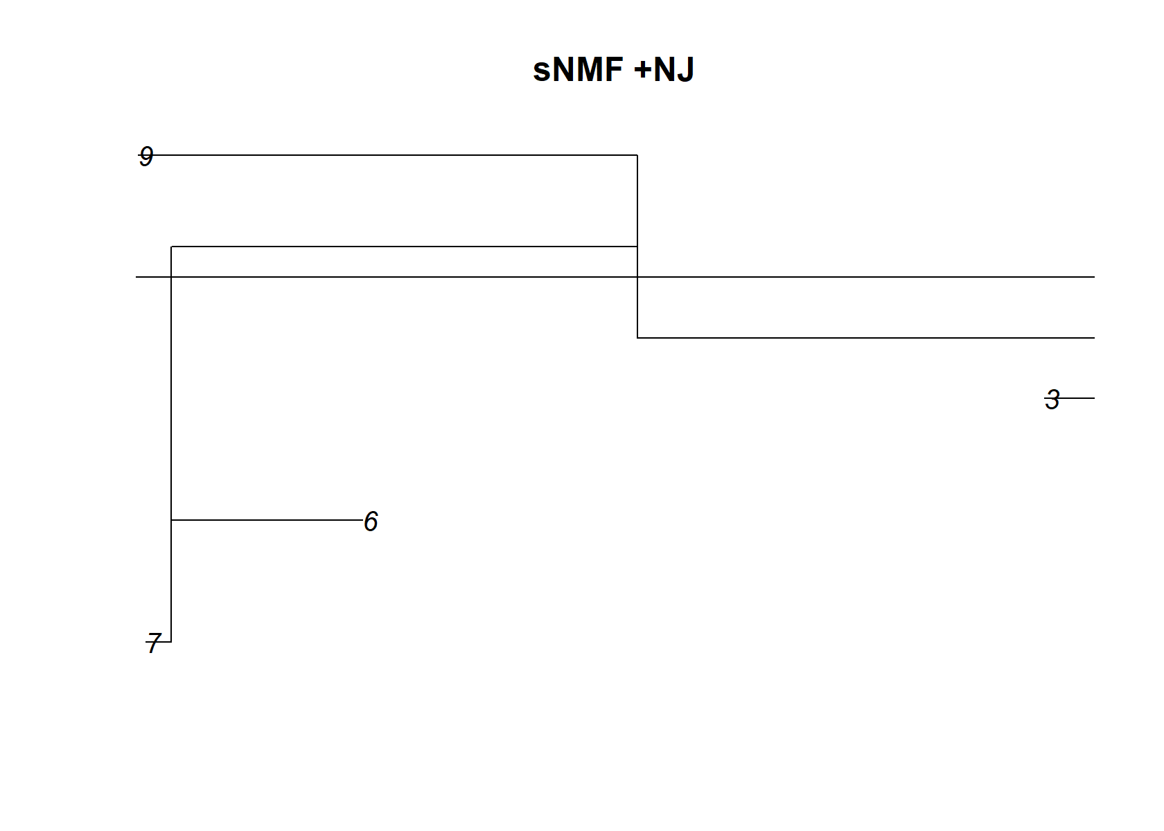
| Version | Author | Date |
|---|---|---|
| 9b5463e | WD | 2024-12-16 |
check_tree$edge.length=abs(check_tree$edge.length)
plot(check_tree)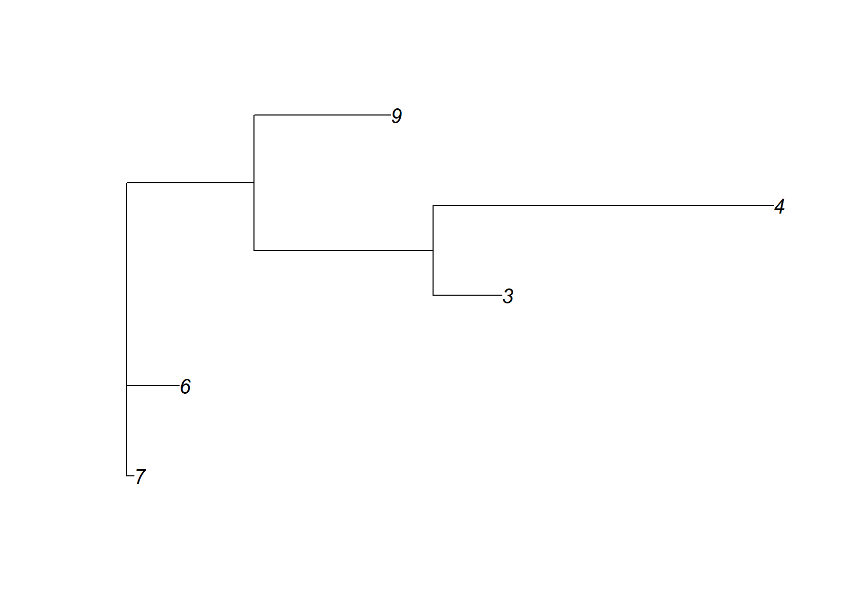
| Version | Author | Date |
|---|---|---|
| 9b5463e | WD | 2024-12-16 |
sessionInfo()
# R version 4.4.1 (2024-06-14 ucrt)
# Platform: x86_64-w64-mingw32/x64
# Running under: Windows 11 x64 (build 26100)
#
# Matrix products: default
#
#
# locale:
# [1] LC_COLLATE=English_United States.utf8
# [2] LC_CTYPE=English_United States.utf8
# [3] LC_MONETARY=English_United States.utf8
# [4] LC_NUMERIC=C
# [5] LC_TIME=English_United States.utf8
#
# time zone: Europe/Oslo
# tzcode source: internal
#
# attached base packages:
# [1] stats     graphics  grDevices utils     datasets  methods   base
#
# other attached packages:
# [1] ape_5.8            cowplot_1.1.3      ggplot2_3.5.1      fastTopics_0.6-192
# [5] Matrix_1.7-0
#
# loaded via a namespace (and not attached):
#  [1] gtable_0.3.6        xfun_0.49           bslib_0.8.0
#  [4] htmlwidgets_1.6.4   ggrepel_0.9.6       lattice_0.22-6
#  [7] quadprog_1.5-8      vctrs_0.6.5         tools_4.4.1
# [10] generics_0.1.3      parallel_4.4.1      tibble_3.2.1
# [13] fansi_1.0.6         pkgconfig_2.0.3     data.table_1.16.2
# [16] SQUAREM_2021.1      RcppParallel_5.1.9  lifecycle_1.0.4
# [19] truncnorm_1.0-9     farver_2.1.2        compiler_4.4.1
# [22] stringr_1.5.1       git2r_0.35.0        progress_1.2.3
# [25] munsell_0.5.1       RhpcBLASctl_0.23-42 httpuv_1.6.15
# [28] htmltools_0.5.8.1   sass_0.4.9          yaml_2.3.10
# [31] lazyeval_0.2.2      plotly_4.10.4       crayon_1.5.3
# [34] later_1.4.1         pillar_1.9.0        jquerylib_0.1.4
# [37] whisker_0.4.1       tidyr_1.3.1         uwot_0.2.2
# [40] cachem_1.1.0        nlme_3.1-164        gtools_3.9.5
# [43] tidyselect_1.2.1    digest_0.6.37       Rtsne_0.17
# [46] stringi_1.8.4       dplyr_1.1.4         purrr_1.0.2
# [49] ashr_2.2-63         labeling_0.4.3      rprojroot_2.0.4
# [52] fastmap_1.2.0       grid_4.4.1          colorspace_2.1-1
# [55] cli_3.6.3           invgamma_1.1        magrittr_2.0.3
# [58] utf8_1.2.4          withr_3.0.2         prettyunits_1.2.0
# [61] scales_1.3.0        promises_1.3.2      rmarkdown_2.29
# [64] httr_1.4.7          workflowr_1.7.1     hms_1.1.3
# [67] pbapply_1.7-2       evaluate_1.0.1      knitr_1.49
# [70] viridisLite_0.4.2   irlba_2.3.5.1       rlang_1.1.4
# [73] Rcpp_1.0.13         mixsqp_0.3-54       glue_1.7.0
# [76] rstudioapi_0.17.1   jsonlite_1.8.8      R6_2.5.1
# [79] fs_1.6.5