DE analysis using a topic model: evaluation using simulated data
Peter Carbonetto
Last updated: 2021-10-15
Checks: 6 1
Knit directory: single-cell-topics/analysis/
This reproducible R Markdown analysis was created with workflowr (version 1.6.2). The Checks tab describes the reproducibility checks that were applied when the results were created. The Past versions tab lists the development history.
Great! Since the R Markdown file has been committed to the Git repository, you know the exact version of the code that produced these results.
Great job! The global environment was empty. Objects defined in the global environment can affect the analysis in your R Markdown file in unknown ways. For reproduciblity it’s best to always run the code in an empty environment.
The command set.seed(1) was run prior to running the code in the R Markdown file. Setting a seed ensures that any results that rely on randomness, e.g. subsampling or permutations, are reproducible.
Great job! Recording the operating system, R version, and package versions is critical for reproducibility.
- de-noshrink
- de-with-ash
- fit-poisson-nmf
To ensure reproducibility of the results, delete the cache directory de_analysis_detailed_look_cache and re-run the analysis. To have workflowr automatically delete the cache directory prior to building the file, set delete_cache = TRUE when running wflow_build() or wflow_publish().
Great job! Using relative paths to the files within your workflowr project makes it easier to run your code on other machines.
Great! You are using Git for version control. Tracking code development and connecting the code version to the results is critical for reproducibility.
The results in this page were generated with repository version afaa55d. See the Past versions tab to see a history of the changes made to the R Markdown and HTML files.
Note that you need to be careful to ensure that all relevant files for the analysis have been committed to Git prior to generating the results (you can use wflow_publish or wflow_git_commit). workflowr only checks the R Markdown file, but you know if there are other scripts or data files that it depends on. Below is the status of the Git repository when the results were generated:
Ignored files:
    Ignored:    data/droplet.RData
    Ignored:    data/pbmc_68k.RData
    Ignored:    data/pbmc_purified.RData
    Ignored:    data/pulseseq.RData
    Ignored:    output/droplet/diff-count-droplet.RData
    Ignored:    output/droplet/fits-droplet.RData
    Ignored:    output/droplet/rds/
    Ignored:    output/pbmc-68k/fits-pbmc-68k.RData
    Ignored:    output/pbmc-68k/rds/
    Ignored:    output/pbmc-purified/fits-pbmc-purified.RData
    Ignored:    output/pbmc-purified/rds/
    Ignored:    output/pulseseq/diff-count-pulseseq.RData
    Ignored:    output/pulseseq/fits-pulseseq.RData
    Ignored:    output/pulseseq/rds/

Untracked files:
    Untracked:  analysis/de_analysis_detailed_look_cache/
    Untracked:  plots/
Note that any generated files, e.g. HTML, png, CSS, etc., are not included in this status report because it is ok for generated content to have uncommitted changes.
These are the previous versions of the repository in which changes were made to the R Markdown (analysis/de_analysis_detailed_look.Rmd) and HTML (docs/de_analysis_detailed_look.html) files. If you’ve configured a remote Git repository (see ?wflow_git_remote), click on the hyperlinks in the table below to view the files as they were in that past version.
| File | Version | Author | Date | Message |
|---|---|---|---|---|
| Rmd | afaa55d | Peter Carbonetto | 2021-10-15 | workflowr::wflow_publish(“de_analysis_detailed_look.Rmd”) |
| Rmd | 13d2f7d | Peter Carbonetto | 2021-10-14 | Added pvalue/lfsr histograms for deseq2 and fastTopics. |
| Rmd | 09089ff | Peter Carbonetto | 2021-10-14 | Revising de_analysis_detailed_look after fixing z-score calculations in de_analysis. |
| html | f61da64 | Peter Carbonetto | 2021-10-14 | Fixed a bug in the power vs fdr plot in de_analysis_detailed_look. |
| Rmd | cb60f4c | Peter Carbonetto | 2021-10-14 | workflowr::wflow_publish(“de_analysis_detailed_look.Rmd”) |
| html | 3d62d9e | Peter Carbonetto | 2021-10-14 | Revised plots and explanatory text in de_analysis_detailed_look. |
| Rmd | 5d5c6a6 | Peter Carbonetto | 2021-10-14 | workflowr::wflow_publish(“de_analysis_detailed_look.Rmd”) |
| html | 468f4d9 | Peter Carbonetto | 2021-10-13 | Added draft plots to de_analysis_detailed_look investigation. |
| Rmd | eceb899 | Peter Carbonetto | 2021-10-13 | workflowr::wflow_publish(“de_analysis_detailed_look.Rmd”, verbose = TRUE) |
| html | 7236187 | Peter Carbonetto | 2021-10-13 | Revised the data simulation and added some “shrink vs. noshrink” plots |
| Rmd | 6d63993 | Peter Carbonetto | 2021-10-13 | Made another simplification to simulate_twotopic_umi_data and added plots to de_analysis_detailed_look analysis comparing results with and without shrinkage. |
| Rmd | 157f7d3 | Peter Carbonetto | 2021-10-12 | Working on improved script driving_genes_better.R. |
| html | af856a2 | Peter Carbonetto | 2021-10-12 | Fixed the plots showing properties of the simulated data in the |
| Rmd | 2726a86 | Peter Carbonetto | 2021-10-12 | workflowr::wflow_publish(“de_analysis_detailed_look.Rmd”) |
| html | b8eadee | Peter Carbonetto | 2021-10-11 | Added some basic histograms to the de_analysis_detailed_look analysis. |
| Rmd | e2577f1 | Peter Carbonetto | 2021-10-11 | Working on the data simulation step in the de_analysis_detailed_look |
| html | cd17ccf | Peter Carbonetto | 2021-10-09 | Initial build of the de_analysis_detailed_look workflowr page. |
| Rmd | b8e1fe8 | Peter Carbonetto | 2021-10-09 | workflowr::wflow_publish(“de_analysis_detailed_look.Rmd”) |
| Rmd | 888ea7d | Peter Carbonetto | 2021-10-08 | I have an initial implementation of function simulate_twotopic_scrnaseq_data used to evaluate the de_analysis methods in fastTopics. |
Add summary of the analysis here.
Load the packages used in the analysis below, and some additional functions for simulating the data.
library(Matrix)
library(scran)
# Warning: package 'S4Vectors' was built under R version 3.6.3
# Warning: package 'GenomeInfoDb' was built under R version 3.6.3
# Warning: package 'DelayedArray' was built under R version 3.6.3
library(DESeq2)
library(fastTopics)
library(ggplot2)
library(cowplot)
source("../code/de_eval_functions.R")
Simulate UMI counts
We begin by simulating counts from a rank-2 Poisson NMF model with parameters chosen to roughly mimic the UMI counts from a single-cell RNA sequencing experiment. For now, we focus our attention on the rank-2 (i.e., two topics) case to simplify the evaluation of the DE methods; comparing gene expression between three or topics brings some additional complications which aren’t necessary for assessing basic properties of the new DE methods. For more details on how the data are simulated, see function simulate_twotopic_umi_data.
set.seed(1)
dat <- simulate_twotopic_umi_data()
X <- dat$X
F <- dat$F
L <- dat$L
Before fitting a topic model and running a DE analysis, we first inspect some basic properties of the simulated data.
The sample sizes (total counts for each cell) are roughly normal on the (base-10) log scale:
s <- rowSums(X)
p1 <- ggplot(data.frame(s = log10(s)),aes(x = s)) +
  geom_histogram(color = "white",fill = "black",bins = 32) +
  labs(x = "log10 size",y = "cells") +
  theme_cowplot()
print(p1)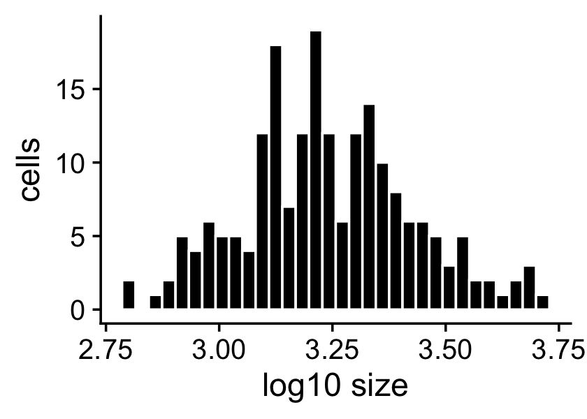
The expression rates were simulated so that they are normally distributed on the log scale:
p2 <- ggplot(data.frame(f = as.vector(F)),aes(x = log10(f))) +
  geom_histogram(color = "white",fill = "black",bins = 32) +
  labs(x = "log10 expression rate",y = "genes") +
  theme_cowplot()
print(p2)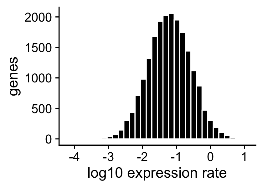
About half of the genes have nonzero differences in expression between the two topics. Among the nonzero gene expression differences, the log-fold changes (LFCs) were simulated from the normal distribution:
nonzero_lfc <- abs(F[,1] - F[,2]) > 1e-8
lfc <- log2(F[,2]/F[,1])
p3 <- ggplot(data.frame(lfc = lfc[nonzero_lfc]),aes(x = lfc)) +
  geom_histogram(color = "white",fill = "black",bins = 32) +
  labs(x = "LFC",y = "genes") +
  theme_cowplot()
print(p3)
mean(nonzero_lfc)
# [1] 0.496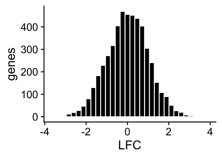
Fit multinomial topic model to UMI counts
Here we fit a multinomial topic model to the simulated UMI count data. To simplify evaluation of the DE methods, we assume that the topic proportions are known, and set them to their ground truth values (that is, the values used to simulate the data). In this way, the only error that can arise is in the estimates of the expression rates \(f_{ij}\).
fit0 <- init_poisson_nmf(X,F = dat$F,L = with(dat,s*L))
fit <- fit_poisson_nmf(X,fit0 = fit0,numiter = 40,method = "scd",
                       update.loadings = NULL,verbose = "none")
fit <- poisson2multinom(fit)
summary(fit)
# Model overview:
#   Number of data rows, n: 200
#   Number of data cols, m: 10000
#   Rank/number of topics, k: 2
# Evaluation of model fit (40 updates performed):
#   Poisson NMF log-likelihood: -7.169037374429e+05
#   Multinomial topic model log-likelihood: -7.158926302076e+05
#   Poisson NMF deviance: +8.564731575439e+05
#   Max KKT residual: +4.123695e-06
Warning: The above code chunk cached its results, but it won’t be re-run if previous chunks it depends on are updated. If you need to use caching, it is highly recommended to also set knitr::opts_chunk$set(autodep = TRUE) at the top of the file (in a chunk that is not cached). Alternatively, you can customize the option dependson for each individual chunk that is cached. Using either autodep or dependson will remove this warning. See the knitr cache options for more details.
DE analysis with and without shrinkage
First we perform a DE analysis without shrinking the LFC estimates:
set.seed(1)
de.noshrink <- de_analysis(fit,X,shrink.method = "none",
                           control = list(ns = 1e4,nc = 2))
# Fitting 10000 Poisson models with k=2 using method="scd".
# Computing log-fold change statistics from 10000 Poisson models with k=2.
Warning: The above code chunk cached its results, but it won’t be re-run if previous chunks it depends on are updated. If you need to use caching, it is highly recommended to also set knitr::opts_chunk$set(autodep = TRUE) at the top of the file (in a chunk that is not cached). Alternatively, you can customize the option dependson for each individual chunk that is cached. Using either autodep or dependson will remove this warning. See the knitr cache options for more details.
Now we perform a second DE analysis using adaptive shrinkage to shrink (and hopefully improve accuracy of) the LFC estimates:
set.seed(1)
de <- de_analysis(fit,X,shrink.method = "ash",control = list(ns = 1e4,nc = 2))
# Fitting 10000 Poisson models with k=2 using method="scd".
# Computing log-fold change statistics from 10000 Poisson models with k=2.
# Stabilizing posterior log-fold change estimates using adaptive shrinkage.
Warning: The above code chunk cached its results, but it won’t be re-run if previous chunks it depends on are updated. If you need to use caching, it is highly recommended to also set knitr::opts_chunk$set(autodep = TRUE) at the top of the file (in a chunk that is not cached). Alternatively, you can customize the option dependson for each individual chunk that is cached. Using either autodep or dependson will remove this warning. See the knitr cache options for more details.
In this scatterplot, we compare the posterior mean LFC estimates with and without performing the shrinkage step. As expected, the smaller LFC estimates, or the LFC estimates corresponding to genes with lower expression, tend to be more strongly shrunk toward zero.
pdat <- data.frame(noshrink  = de.noshrink$postmean[,2],
                   shrink    = de$postmean[,2],
                   log10mean = log10(de$f0))
p4 <- ggplot(pdat,aes(x = noshrink,y = shrink,fill = log10mean)) +
  geom_point(shape = 21,color = "white",size = 2) +
  geom_abline(intercept = 0,slope = 1,color = "black",linetype = "dotted") +
  scale_fill_gradient2(low = "deepskyblue",mid = "gold",high = "orangered",
                       midpoint = -4) +
  labs(x = "original LFC estimates",
       y = "shrunken LFC estimates") +
  theme_cowplot()
print(p4)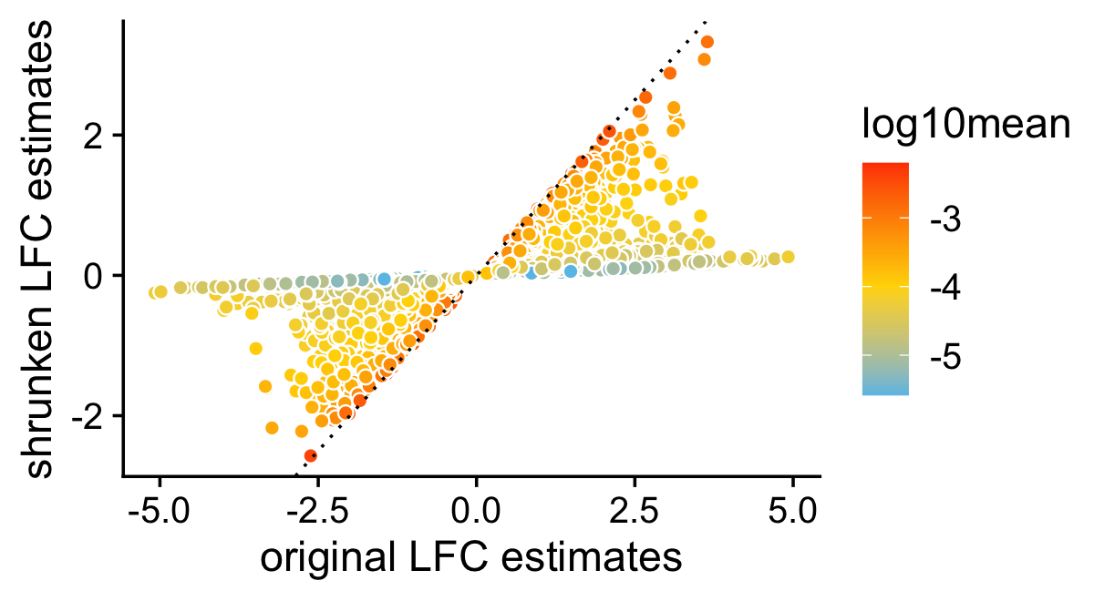
These next two bar charts show the overall impact of the shrinkage on the distribution of the \(z\)-scores; dark blue bars are for diifferentially expressed genes, and orange bars are for non-differentially expressed genes.
pdat <- data.frame(noshrink = clamp(de.noshrink$z[,2],-8,+8),
                   shrink   = clamp(de$z[,2],-8,+8),
                   de       = factor(nonzero_lfc))
p5 <- ggplot(pdat,aes(x = noshrink,color = de,fill = de)) +
  geom_histogram(bins = 64) +
  scale_color_manual(values = c("darkorange","darkblue")) +
  scale_fill_manual(values = c("darkorange","darkblue")) +
  labs(x = "z-score",y = "genes",title = "without shrinkage") +
  theme_cowplot()
p6 <- ggplot(pdat,aes(x = shrink,color = de,fill = de)) +
  geom_histogram(bins = 64) +
  scale_color_manual(values = c("darkorange","darkblue")) +
  scale_fill_manual(values = c("darkorange","darkblue")) +
  labs(x = "z-score",y = "genes",title = "with shrinkage") +
  theme_cowplot()
print(plot_grid(p5,p6))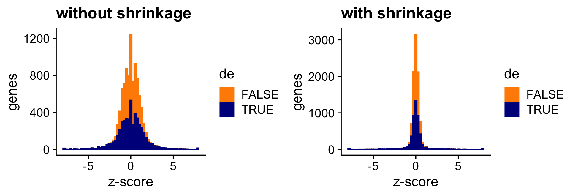
And the next two bar charts show the overall impact of the shrinkage on the \(p\)-values.
pdat <- data.frame(noshrink = 10^(-de.noshrink$lpval[,2]),
                   shrink   = 10^(-de$lpval[,2]),
                   de       = factor(nonzero_lfc))
p7 <- ggplot(pdat,aes(x = noshrink,color = de,fill = de)) +
  geom_histogram(bins = 64) +
  scale_color_manual(values = c("darkorange","darkblue")) +
  scale_fill_manual(values = c("darkorange","darkblue")) +
  labs(x = "p-value",y = "genes",title = "without shrinkage") +
  theme_cowplot()
p8 <- ggplot(pdat,aes(x = shrink,color = de,fill = de)) +
  geom_histogram(bins = 64) +
  scale_color_manual(values = c("darkorange","darkblue")) +
  scale_fill_manual(values = c("darkorange","darkblue")) +
  labs(x = "p-value",y = "genes",title = "with shrinkage") +
  theme_cowplot()
print(plot_grid(p7,p8))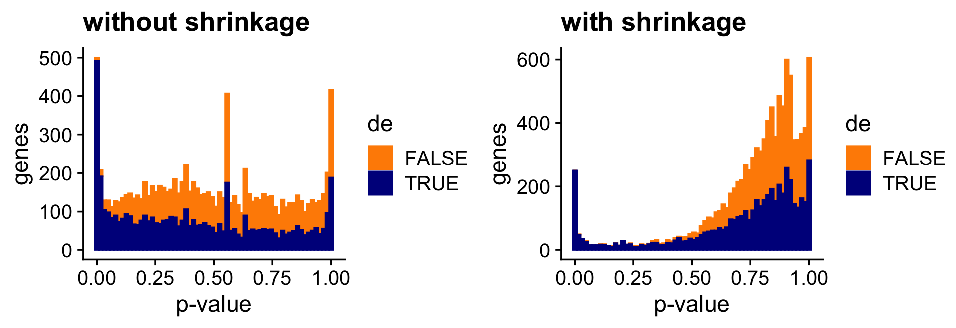
Quantifying uncertainty in the LFC estimates
Above, we assessed the usefulness of applying the adaptive shrinkage method to improve the accuracy of the LFC estimates. This idea of shrinking the LFC estimates is not new, and is already implemented in DESeq2, also using adaptive shrinkage.
A more important aspect of the DE analysis methods in fastTopics is that it quantifies uncertainty in the LFC estimates by computing posterior HPD intervals. To see why this is important, consider this plot compare the point estimates (specifically, MLEs) of the LFCs (X axis) against the shrunken posterior mean estimates (Y axis). What is striking is that even very large (in magnitude) point estimates can be shrunk to zero; this happens because although the MLEs can be far from zero, the HPD intervals are also very large.
pdat <- data.frame(est       = de$est[,2],
                   shrink    = de$postmean[,2],
                   log10mean = log10(de$f0))
p9 <- ggplot(pdat,aes(x = est,y = shrink,fill = log10mean)) +
  geom_point(shape = 21,color = "white",size = 2) +
  geom_abline(intercept = 0,slope = 1,color = "black",linetype = "dotted") +
  scale_fill_gradient2(low = "deepskyblue",mid = "gold",high = "orangered",
                       midpoint = -4) +
  labs(x = "point estimates",
       y = "shrunken estimates") +
  theme_cowplot()
print(p9)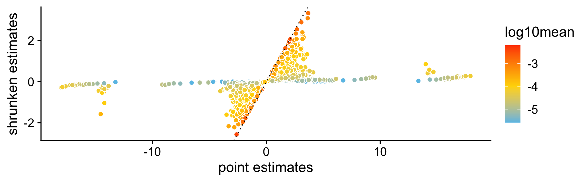
To illustrate the impact of this on the DE analysis, consider the K-L divergence measure used in Dey, Hsiao & Stephens (2017) to rank genes, which doesn’t fully account for uncertainty in the LFCs. As a result, sometimes genes with very large LFCs get highly ranked, but after a full accounting for uncertainty, they are no longer ranked highly.
i     <- which(fit$F[,2] - fit$F[,1] > -1e-8)
D     <- fastTopics:::min_kl_poisson(fit$F)
pdat1 <- data.frame(kl = pmin(D[,2],0.00025),de = factor(nonzero_lfc))
pdat2 <- data.frame(z = clamp(de$z[,2],-4,+4),de = factor(nonzero_lfc))
pdat1 <- pdat1[i,]
pdat2 <- pdat2[i,]
p10 <- ggplot(pdat1,aes(x = kl,color = de,fill = de)) +
  geom_histogram(bins = 64) +
  scale_x_continuous(breaks = c(0,0.0001,0.0002)) +
  scale_color_manual(values = c("darkorange","darkblue")) +
  scale_fill_manual(values = c("darkorange","darkblue")) +
  labs(x = "K-L divergence",y = "genes") +
  theme_cowplot()
p11 <- ggplot(pdat2,aes(x = z,color = de,fill = de)) +
  geom_histogram(bins = 64) +
  scale_color_manual(values = c("darkorange","darkblue")) +
  scale_fill_manual(values = c("darkorange","darkblue")) +
  labs(x = "z-score",y = "genes") +
  theme_cowplot()
print(plot_grid(p10,p11))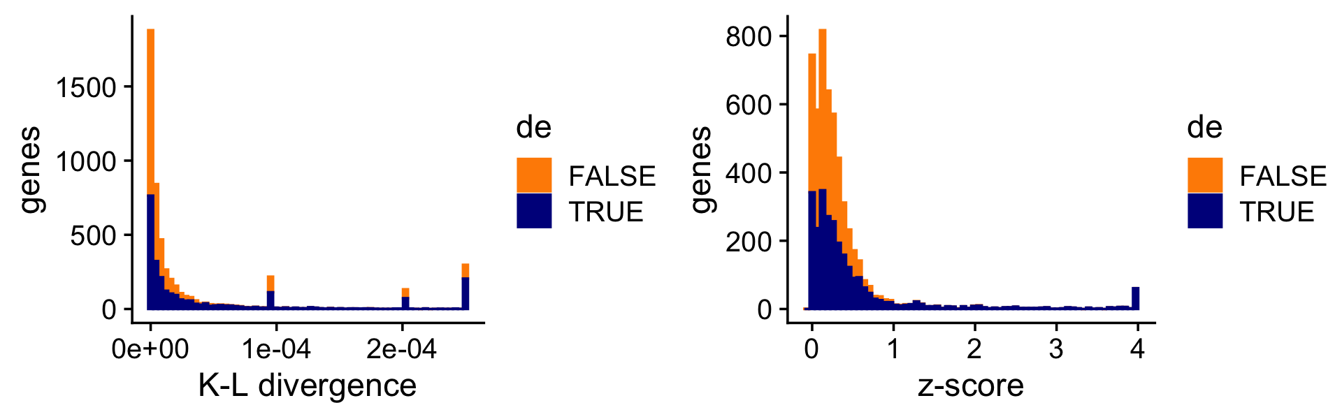
To drive home this point, suppose we used the KL-divergences and the p-values returned by de_analysis(shrink.method = "ash") to discover differentially expressed genes. The power vs. FDR curves show that the rankings accounting for uncertainty in the LFC estimates (with or without shrinkage) perform better than the ranking based on the KL divergence measure.
pdat1 <- create_fdr_vs_power_curve(-D[,2],nonzero_lfc)
pdat2 <- create_fdr_vs_power_curve(-de.noshrink$lpval[,2],nonzero_lfc)
pdat3 <- create_fdr_vs_power_curve(-de$lpval[,2],nonzero_lfc)
pdat  <- rbind(cbind(pdat1,method = "kl"),
               cbind(pdat2,method = "noshrink"),
               cbind(pdat3,method = "shrink"))
p12 <- ggplot(pdat,aes(x = fdr,y = power,color = method)) +
  geom_point(size = 0.75)  +
  scale_color_manual(values = c("royalblue","limegreen","darkorange")) +
  theme_cowplot()
print(p12)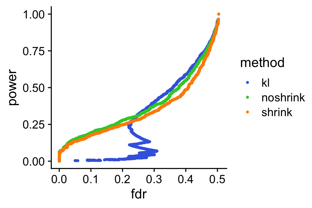
Comparison with DESeq2
Add text and code here.
i       <- which(apply(L,1,max) > 0.99)
Y       <- t(X[i,])
cluster <- factor(apply(L,1,which.max))
deseq   <- DESeqDataSetFromMatrix(Y,data.frame(cluster = cluster[i]),~cluster)
# converting counts to integer mode
sizeFactors(deseq) <- calculateSumFactors(Y)
deseq <- DESeq(deseq,test = "LRT",reduced=~1,useT = TRUE,minmu = 1e-6,
               minReplicatesForReplace = Inf)
# using pre-existing size factors
# estimating dispersions
# gene-wise dispersion estimates
# mean-dispersion relationship
# -- note: fitType='parametric', but the dispersion trend was not well captured by the
#    function: y = a/x + b, and a local regression fit was automatically substituted.
#    specify fitType='local' or 'mean' to avoid this message next time.
# final dispersion estimates
# fitting model and testing
deseq <- lfcShrink(deseq,coef = "cluster_2_vs_1",type = "ashr")
# using 'ashr' for LFC shrinkage. If used in published research, please cite:
#     Stephens, M. (2016) False discovery rates: a new deal. Biostatistics, 18:2.
#     https://doi.org/10.1093/biostatistics/kxw041
z.deseq <- with(deseq,log2FoldChange/lfcSE)
Add text here.
plot(deseq$log2FoldChange,de$postmean[,2],pch = 20,col = "royalblue")
abline(a = 0,b = 1,col = "black",lty = "dotted")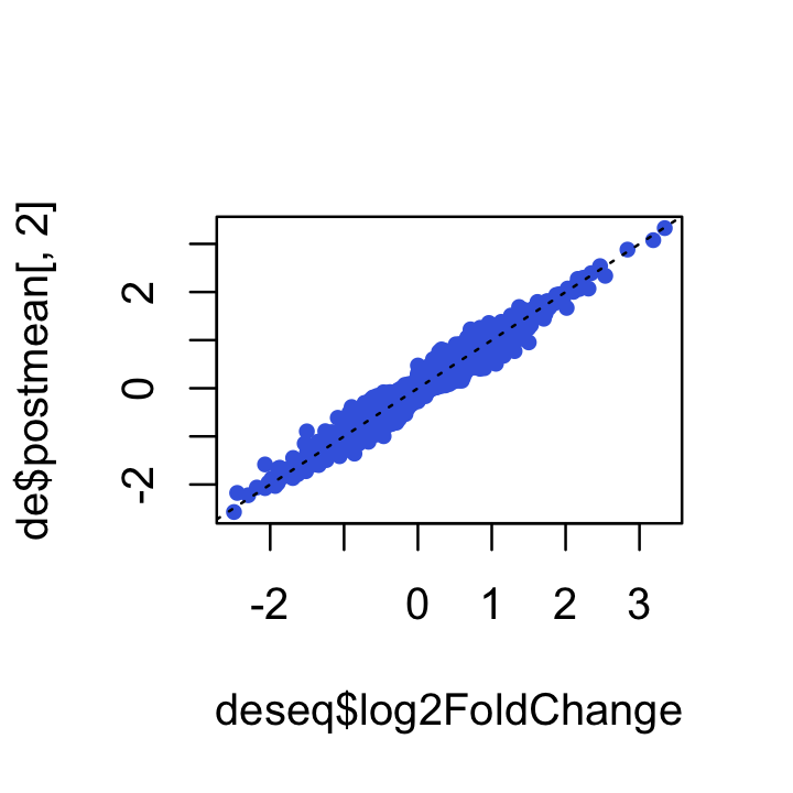
plot(z.deseq,de$z[,2],pch = 20,col = "royalblue")
abline(a = 0,b = 1,col = "black",lty = "dotted")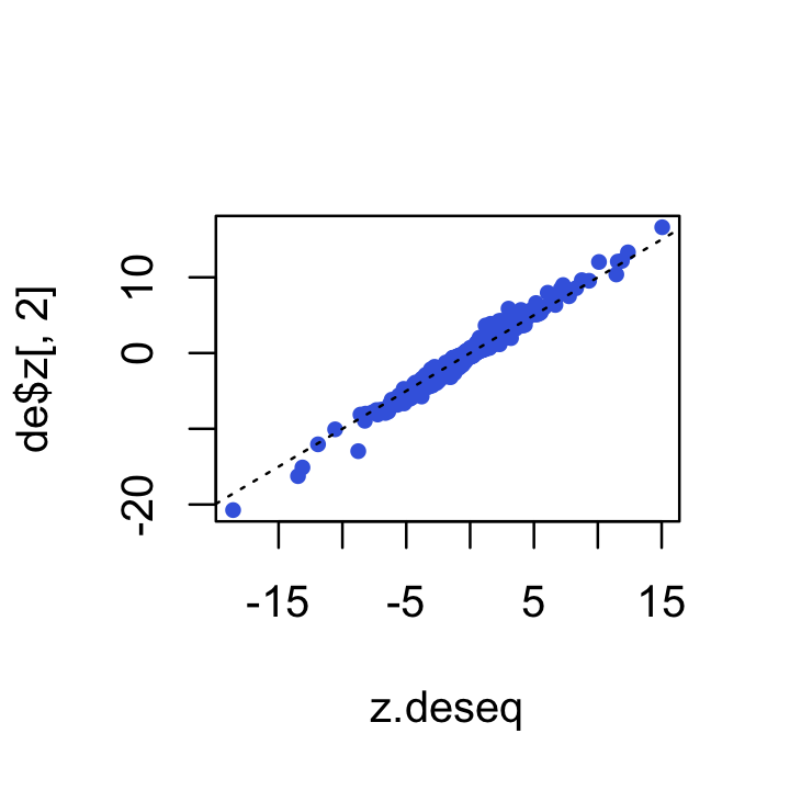
Add text here.
pdat <- data.frame(deseq2 = deseq$padj,
                   shrink = de$lfsr[,2],
                   de     = factor(nonzero_lfc))
p1 <- ggplot(pdat,aes(x = deseq2,color = de,fill = de)) +
  geom_histogram(bins = 64) +
  scale_color_manual(values = c("darkorange","darkblue")) +
  scale_fill_manual(values = c("darkorange","darkblue")) +
  labs(x = "p-value",y = "genes",title = "deseq with shrinkage") +
  theme_cowplot() +
  theme(plot.title = element_text(size = 12,face = "plain"))
p2 <- ggplot(pdat,aes(x = shrink,color = de,fill = de)) +
  geom_histogram(bins = 64) +
  scale_color_manual(values = c("darkorange","darkblue")) +
  scale_fill_manual(values = c("darkorange","darkblue")) +
  labs(x = "lfsr",y = "genes",
       title = "de_analysis(shrink.method = \"ash\")") +
  theme_cowplot() +
  theme(plot.title = element_text(size = 12,face = "plain"))
print(plot_grid(p1,p2))
# Warning: Removed 3326 rows containing non-finite values (stat_bin).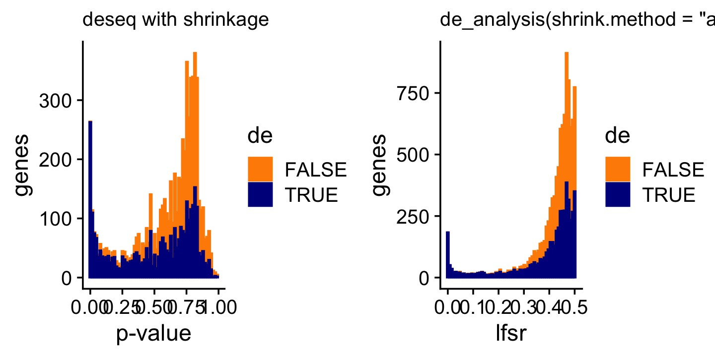
TO DO: Add power vs. FDR plots comparing DESeq2 and fastTopics.
sessionInfo()
# R version 3.6.2 (2019-12-12)
# Platform: x86_64-apple-darwin15.6.0 (64-bit)
# Running under: macOS Catalina 10.15.7
#
# Matrix products: default
# BLAS:   /Library/Frameworks/R.framework/Versions/3.6/Resources/lib/libRblas.0.dylib
# LAPACK: /Library/Frameworks/R.framework/Versions/3.6/Resources/lib/libRlapack.dylib
#
# locale:
# [1] en_US.UTF-8/en_US.UTF-8/en_US.UTF-8/C/en_US.UTF-8/en_US.UTF-8
#
# attached base packages:
# [1] parallel  stats4    stats     graphics  grDevices utils     datasets
# [8] methods   base
#
# other attached packages:
#  [1] cowplot_1.0.0               ggplot2_3.3.5
#  [3] fastTopics_0.6-73           DESeq2_1.33.5
#  [5] scran_1.14.6                SingleCellExperiment_1.8.0
#  [7] SummarizedExperiment_1.16.1 DelayedArray_0.12.3
#  [9] BiocParallel_1.18.1         matrixStats_0.56.0
# [11] Biobase_2.46.0              GenomicRanges_1.38.0
# [13] GenomeInfoDb_1.22.1         IRanges_2.20.2
# [15] S4Vectors_0.24.4            BiocGenerics_0.32.0
# [17] Matrix_1.2-18
#
# loaded via a namespace (and not attached):
#   [1] Rtsne_0.15               ggbeeswarm_0.6.0         colorspace_1.4-1
#   [4] ellipsis_0.3.2           rprojroot_1.3-2          XVector_0.26.0
#   [7] BiocNeighbors_1.2.0      fs_1.3.1                 farver_2.0.1
#  [10] MatrixModels_0.4-1       ggrepel_0.9.1            bit64_0.9-7
#  [13] AnnotationDbi_1.48.0     fansi_0.4.0              splines_3.6.2
#  [16] geneplotter_1.64.0       knitr_1.26               scater_1.14.6
#  [19] jsonlite_1.7.2           workflowr_1.6.2          mcmc_0.9-6
#  [22] annotate_1.64.0          ashr_2.2-51              httr_1.4.2
#  [25] compiler_3.6.2           dqrng_0.2.1              backports_1.1.5
#  [28] lazyeval_0.2.2           assertthat_0.2.1         limma_3.42.2
#  [31] later_1.0.0              BiocSingular_1.2.2       prettyunits_1.1.1
#  [34] htmltools_0.4.0          quantreg_5.54            tools_3.6.2
#  [37] rsvd_1.0.2               igraph_1.2.5             coda_0.19-3
#  [40] gtable_0.3.0             glue_1.4.2               GenomeInfoDbData_1.2.2
#  [43] dplyr_1.0.7              Rcpp_1.0.7               vctrs_0.3.8
#  [46] DelayedMatrixStats_1.6.1 xfun_0.11                stringr_1.4.0
#  [49] lifecycle_1.0.0          irlba_2.3.3              statmod_1.4.34
#  [52] XML_3.99-0.3             edgeR_3.28.1             zlibbioc_1.32.0
#  [55] MASS_7.3-51.4            scales_1.1.0             hms_1.1.0
#  [58] promises_1.1.0           SparseM_1.78             RColorBrewer_1.1-2
#  [61] yaml_2.2.0               memoise_1.1.0            gridExtra_2.3
#  [64] stringi_1.4.3            RSQLite_2.2.0            SQUAREM_2017.10-1
#  [67] genefilter_1.68.0        truncnorm_1.0-8          rlang_0.4.11
#  [70] pkgconfig_2.0.3          bitops_1.0-6             invgamma_1.1
#  [73] evaluate_0.14            lattice_0.20-38          purrr_0.3.4
#  [76] labeling_0.3             htmlwidgets_1.5.1        bit_1.1-15.2
#  [79] tidyselect_1.1.1         magrittr_2.0.1           R6_2.4.1
#  [82] generics_0.0.2           DBI_1.1.0                withr_2.4.2
#  [85] pillar_1.6.2             whisker_0.4              mixsqp_0.3-46
#  [88] survival_3.1-8           RCurl_1.98-1.2           tibble_3.1.3
#  [91] crayon_1.4.1             utf8_1.1.4               plotly_4.9.2
#  [94] rmarkdown_2.3            progress_1.2.2           viridis_0.5.1
#  [97] locfit_1.5-9.4           grid_3.6.2               data.table_1.12.8
# [100] blob_1.2.1               git2r_0.26.1             digest_0.6.23
# [103] xtable_1.8-4             tidyr_1.1.3              httpuv_1.5.2
# [106] MCMCpack_1.4-5           RcppParallel_4.4.2       munsell_0.5.0
# [109] beeswarm_0.2.3           viridisLite_0.3.0        vipor_0.4.5
# [112] quadprog_1.5-8