Visualize and interpret topics in PBMC data
Peter Carbonetto
Last updated: 2020-08-25
Checks: 7 0
Knit directory: single-cell-topics/analysis/
This reproducible R Markdown analysis was created with workflowr (version 1.6.2.9000). The Checks tab describes the reproducibility checks that were applied when the results were created. The Past versions tab lists the development history.
Great! Since the R Markdown file has been committed to the Git repository, you know the exact version of the code that produced these results.
Great job! The global environment was empty. Objects defined in the global environment can affect the analysis in your R Markdown file in unknown ways. For reproduciblity it’s best to always run the code in an empty environment.
The command set.seed(1) was run prior to running the code in the R Markdown file. Setting a seed ensures that any results that rely on randomness, e.g. subsampling or permutations, are reproducible.
Great job! Recording the operating system, R version, and package versions is critical for reproducibility.
Nice! There were no cached chunks for this analysis, so you can be confident that you successfully produced the results during this run.
Great job! Using relative paths to the files within your workflowr project makes it easier to run your code on other machines.
Great! You are using Git for version control. Tracking code development and connecting the code version to the results is critical for reproducibility.
The results in this page were generated with repository version 1a0c2d8. See the Past versions tab to see a history of the changes made to the R Markdown and HTML files.
Note that you need to be careful to ensure that all relevant files for the analysis have been committed to Git prior to generating the results (you can use wflow_publish or wflow_git_commit). workflowr only checks the R Markdown file, but you know if there are other scripts or data files that it depends on. Below is the status of the Git repository when the results were generated:
Ignored files:
    Ignored:    data/droplet.RData
    Ignored:    data/pbmc_68k.RData
    Ignored:    data/pbmc_purified.RData
    Ignored:    data/pulseseq.RData
    Ignored:    output/droplet/fits-droplet.RData
    Ignored:    output/droplet/rds/
    Ignored:    output/pbmc-68k/fits-pbmc-68k.RData
    Ignored:    output/pbmc-68k/rds/
    Ignored:    output/pbmc-purified/fits-pbmc-purified.RData
    Ignored:    output/pbmc-purified/rds/
    Ignored:    output/pulseseq/fits-pulseseq.RData
    Ignored:    output/pulseseq/rds/
Note that any generated files, e.g. HTML, png, CSS, etc., are not included in this status report because it is ok for generated content to have uncommitted changes.
These are the previous versions of the repository in which changes were made to the R Markdown (analysis/plots_pbmc.Rmd) and HTML (docs/plots_pbmc.html) files. If you’ve configured a remote Git repository (see ?wflow_git_remote), click on the hyperlinks in the table below to view the files as they were in that past version.
| File | Version | Author | Date | Message |
|---|---|---|---|---|
| Rmd | 1a0c2d8 | Peter Carbonetto | 2020-08-25 | workflowr::wflow_publish(“plots_pbmc.Rmd”) |
| html | eac2d23 | Peter Carbonetto | 2020-08-25 | Revised the cross-tab plot, and added notes to plots_pbmc analysis. |
| html | 2d156b8 | Peter Carbonetto | 2020-08-25 | Revised the cross-tab plot, and added notes to plots_pbmc analysis. |
| Rmd | e8971d8 | Peter Carbonetto | 2020-08-25 | workflowr::wflow_publish(“plots_pbmc.Rmd”) |
| Rmd | 9d8bb28 | Peter Carbonetto | 2020-08-25 | Revised structure plot in plots_pbmc. |
| Rmd | 27f6f51 | Peter Carbonetto | 2020-08-25 | A couple small adjustments to the plotting settings in plots_pbmc. |
| html | abb846e | Peter Carbonetto | 2020-08-25 | Added dotplot to compare clusters vs. cell-types. |
| Rmd | 45c3c32 | Peter Carbonetto | 2020-08-25 | workflowr::wflow_publish(“plots_pbmc.Rmd”) |
| html | f53c86c | Peter Carbonetto | 2020-08-24 | Made a few small improvements to plots_pbmc. |
| Rmd | f7c157a | Peter Carbonetto | 2020-08-24 | workflowr::wflow_publish(“plots_pbmc.Rmd”) |
| Rmd | e13c17e | Peter Carbonetto | 2020-08-24 | Removed reordering of 68k fit, and fixed downstream PCA analyses. |
| Rmd | 01a0c8b | Peter Carbonetto | 2020-08-24 | Fixed colours in 68k structure plot. |
| html | a0cb7c6 | Peter Carbonetto | 2020-08-24 | Added 68k fit structure plot to plots_pbmc analysis. |
| Rmd | 5b2fb5c | Peter Carbonetto | 2020-08-24 | workflowr::wflow_publish(“plots_pbmc.Rmd”) |
| html | b6489db | Peter Carbonetto | 2020-08-23 | Re-built plots_pbmc with new PCA plots from 68k fit. |
| Rmd | 89d98ed | Peter Carbonetto | 2020-08-23 | Removed basic_pca_plot in plots.R; working on PCA plots for 68k fit. |
| html | 13ee038 | Peter Carbonetto | 2020-08-23 | Revised notes in plots_pbmc.Rmd. |
| Rmd | e766da5 | Peter Carbonetto | 2020-08-23 | workflowr::wflow_publish(“plots_pbmc.Rmd”) |
| Rmd | dbd5882 | Peter Carbonetto | 2020-08-23 | Added some explanatory text to plots_pbmc.Rmd. |
| html | 97d7e86 | Peter Carbonetto | 2020-08-23 | Fixed subclustering of cluster A in purified PBMC data. |
| Rmd | 005b217 | Peter Carbonetto | 2020-08-23 | workflowr::wflow_publish(“plots_pbmc.Rmd”) |
| html | 59777e7 | Peter Carbonetto | 2020-08-22 | Added table comparing Zheng et al (2017) labeling with clusters in |
| Rmd | 9cd4a08 | Peter Carbonetto | 2020-08-22 | workflowr::wflow_publish(“plots_pbmc.Rmd”) |
| html | c87ddf8 | Peter Carbonetto | 2020-08-22 | Added PBMC purified structure plot with the new clustering (A1, A2, B, |
| Rmd | c6dd5f2 | Peter Carbonetto | 2020-08-22 | workflowr::wflow_publish(“plots_pbmc.Rmd”) |
| html | ce421ae | Peter Carbonetto | 2020-08-22 | A few small revisions to plots_pbmc analysis. |
| Rmd | ddc6de4 | Peter Carbonetto | 2020-08-22 | workflowr::wflow_publish(“plots_pbmc.Rmd”) |
| html | a406a2f | Peter Carbonetto | 2020-08-22 | Added back first PCA plot for 68k pbmc data. |
| Rmd | 8daa131 | Peter Carbonetto | 2020-08-22 | workflowr::wflow_publish(“plots_pbmc.Rmd”) |
| html | 7900d17 | Peter Carbonetto | 2020-08-22 | Revamping the process of defining clusters in plots_pbmc using PCA. |
| Rmd | 14dd774 | Peter Carbonetto | 2020-08-22 | workflowr::wflow_publish(“plots_pbmc.Rmd”) |
| Rmd | 944ce0c | Peter Carbonetto | 2020-08-22 | Working on new PCA plots for purified PBMC c3 subclusters. |
| html | b05232d | Peter Carbonetto | 2020-08-22 | Build site. |
| Rmd | d0e9f6e | Peter Carbonetto | 2020-08-22 | workflowr::wflow_publish(“plots_pbmc.Rmd”) |
| html | fbb0697 | Peter Carbonetto | 2020-08-21 | Build site. |
| Rmd | cdca13e | Peter Carbonetto | 2020-08-21 | workflowr::wflow_publish(“plots_pbmc.Rmd”) |
| html | 216027a | Peter Carbonetto | 2020-08-21 | Re-built plots_pbmc webpage with structure plots. |
| Rmd | 98888b2 | Peter Carbonetto | 2020-08-21 | Added structure plots to plots_pbmc.R. |
| html | 9310993 | Peter Carbonetto | 2020-08-21 | Revised the PCA plots in pbmc_plots. |
| Rmd | 3a746ff | Peter Carbonetto | 2020-08-21 | workflowr::wflow_publish(“plots_pbmc.Rmd”) |
| Rmd | 1091dd0 | Peter Carbonetto | 2020-08-21 | Added code for Ternary plots to plots_pbmc. |
| html | 6d3d7e4 | Peter Carbonetto | 2020-08-20 | Added 68k PCA plots to plots_pbmc. |
| Rmd | 6ec82ca | Peter Carbonetto | 2020-08-20 | workflowr::wflow_publish(“plots_pbmc.Rmd”) |
| html | 38f07a2 | Peter Carbonetto | 2020-08-20 | A few small revisions to the plots_pbmc analysis. |
| Rmd | fd0316f | Peter Carbonetto | 2020-08-20 | workflowr::wflow_publish(“plots_pbmc.Rmd”) |
| html | 606cd97 | Peter Carbonetto | 2020-08-20 | Added basic PCA plots to plots_pbmc. |
| Rmd | 1b41a60 | Peter Carbonetto | 2020-08-20 | workflowr::wflow_publish(“plots_pbmc.Rmd”) |
| html | d6e5d39 | Peter Carbonetto | 2020-08-20 | Added PCA plot with purified PBMC clustering to plots_pbmc analysis. |
| Rmd | 99301a7 | Peter Carbonetto | 2020-08-20 | workflowr::wflow_publish(“plots_pbmc.Rmd”) |
| Rmd | bf23ca0 | Peter Carbonetto | 2020-08-20 | Added manual labeling of purified PBMC data to plots_pbmc analysis. |
| html | 0c1b570 | Peter Carbonetto | 2020-08-20 | First build on plots_pbmc page. |
| Rmd | eb7f776 | Peter Carbonetto | 2020-08-20 | workflowr::wflow_publish(“plots_pbmc.Rmd”) |
Here we closely examine, and compare, the topic modeling results for the two closely related data sets from Zheng et al (2017), the mixture of FACS-purified PBMC data and the “unsorted” 68k PBMC data. The goal is to illustrate how the topic models fitted to these data sets can be used to learn about the structure in the data, including identifying clusters, and interpret the clusters and topics as “cell types” or “gene programs”.
Load the packages used in the analysis below, as well as additional functions that will be used to generate some of the plots.
library(dplyr)
library(fastTopics)
library(ggplot2)
library(cowplot)
source("../code/plots.R")
Mixture of FACS-purified PBMC data
We begin with the mixture of FACS-purified PBMC data. Note that the count data are no longer needed at this stage.
load("../data/pbmc_purified.RData")
samples_purified <- samples
rm(samples,genes,counts)
Load the \(k = 6\) Poisson NMF model fit.
fit_purified <-
  readRDS("../output/pbmc-purified/rds/fit-pbmc-purified-scd-ex-k=6.rds")$fit
Here we explore the structure of the single-cell data as inferred by the topic model. Specifically, we will use PCA to uncover structure in the topic proportions. Although PCA is simple, we will see that it works well, and avoids the complications of the popular t-SNE and UMAP nonlinear dimensionality reduction methods.
fit <- poisson2multinom(fit_purified)
pca <- prcomp(fit$L)$x
Three large clusters are evident from first two PCs (there is also finer-scale structure which we will examine below). We label these clusters as “A”, “B” and “C”.
n   <- nrow(pca)
x   <- rep("C",n)
pc1 <- pca[,"PC1"]
pc2 <- pca[,"PC2"]
x[pc1 + 0.2 > pc2] <- "A"
x[pc2 > 0.25] <- "B"
x[(pc1 + 0.4)^2 + (pc2 + 0.1)^2 < 0.07] <- "C"
samples_purified$cluster <- x
p1 <- pca_plot_with_labels(fit_purified,c("PC1","PC2"),
                           samples_purified$cluster) +
      labs(fill = "cluster")
print(p1)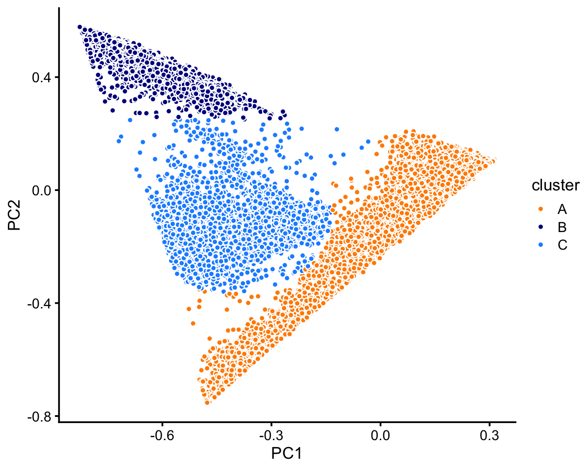
Most of the samples are in cluster A:
table(x)
# x
#     A     B     C
# 72614 10439 11602
Note that other PCs beyond the first two may also sometimes reveal additional clustering, and we will see examples of this in the 68k PBMC data.
Within cluster C there are two fairly well-defined subclusters (labeled “C1” and “C2”). There are perhaps other, less defined subclusters that are less defined, but in this analysis we focus on the largest, most obvious clusters.
rows <- which(samples_purified$cluster == "C")
fit  <- select(poisson2multinom(fit_purified),loadings = rows)
pca  <- prcomp(fit$L)$x
n    <- nrow(pca)
x    <- rep("C3",n)
pc1  <- pca[,1]
pc2  <- pca[,2]
x[pc1 < 0 & pc2 < 0.4] <- "C1"
x[pc1 > 0.5 & pc2 < 0.3] <- "C2"
samples_purified[rows,"cluster"] <- x
p2 <- pca_plot_with_labels(fit,c("PC1","PC2"),x) +
      labs(fill = "cluster")
print(p2)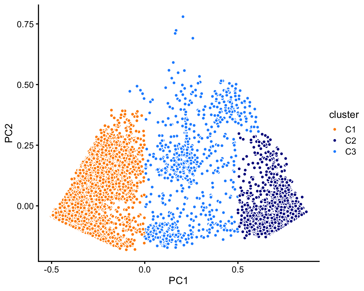
| Version | Author | Date |
|---|---|---|
| 7900d17 | Peter Carbonetto | 2020-08-22 |
The two subclusters, C1 and C2, account for most of the samples in cluster C:
table(x)
# x
#   C1   C2   C3
# 7822 2990  790
Now we turn to cluster A. Within this cluster, there is a large subcluster, which we label as “A1”. (This cluster is much less distinct than the other clusters we have seen so far, and may not show up clearly in this plot—you may need to zoom in on the plot to see the clustering.) Otherwise, there is no obvious additional clustering of the samples within cluster A.
rows <- which(samples_purified$cluster == "A")
fit  <- select(poisson2multinom(fit_purified),loadings = rows)
pca  <- prcomp(fit$L)$x
n    <- nrow(fit$L)
x    <- rep("A2",n)
pc1  <- pca[,1]
pc2  <- pca[,2]
x[pc1 > 0.58 - pc2 | pc1 > 0.7] <- "A1"
samples_purified[rows,"cluster"] <- x
p3 <- pca_plot_with_labels(fit,c("PC1","PC2"),x) +
      labs(fill = "cluster")
print(p3)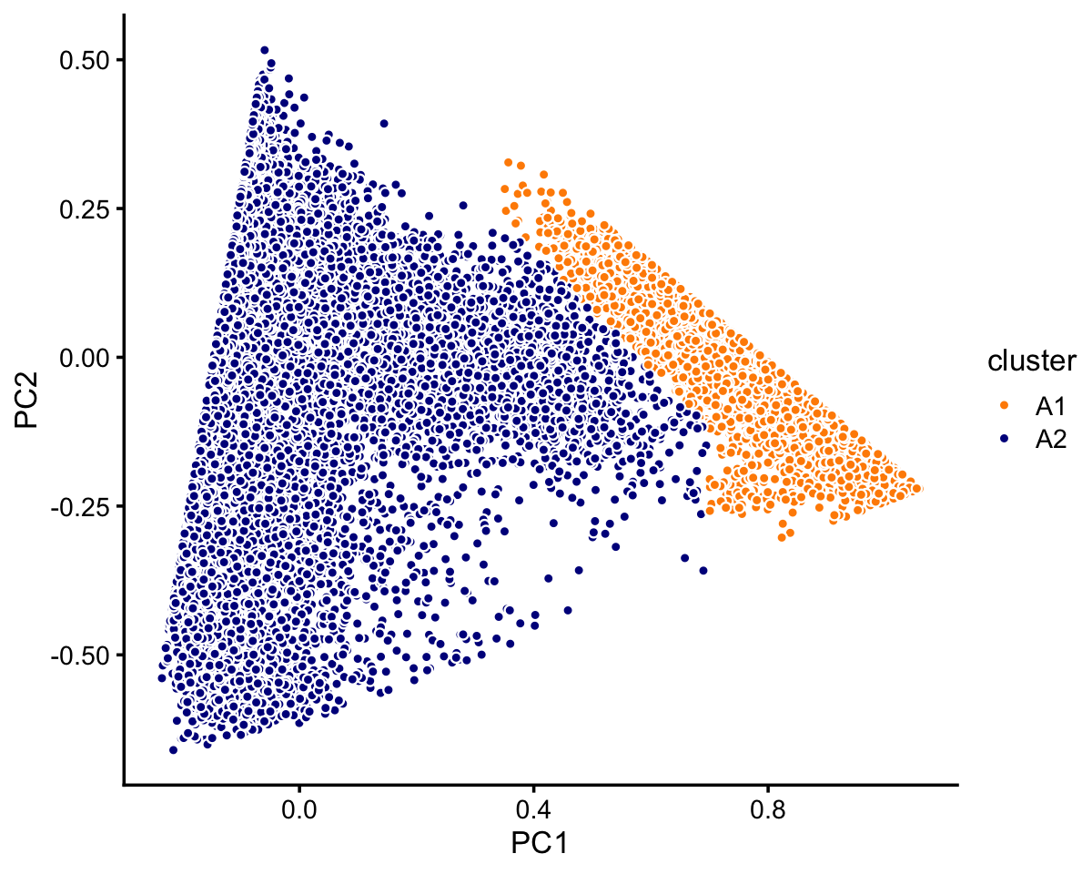
In summary, we have subdivided the data into 6 clusters:
samples_purified$cluster <- factor(samples_purified$cluster)
table(samples_purified$cluster)
#
#    A1    A2     B    C1    C2    C3
#  8271 64343 10439  7822  2990   790
We also inspected principal components individually in each of these 6 clusters and we did not find any of clear examples of subclustering withing these clusters.
The structure plot summarizes the topic proportions in each of these 6 clusters:
set.seed(1)
pbmc_purified_topic_colors <- c("gold","forestgreen","dodgerblue",
                                "gray","greenyellow","magenta")
pbmc_purified_topics <- c(2,5,3,1,4,6)
rows <- sort(c(sample(which(samples_purified$cluster == "A1"),250),
               sample(which(samples_purified$cluster == "A2"),1200),
               sample(which(samples_purified$cluster == "B"),250),
               sample(which(samples_purified$cluster == "C1"),250),
               sample(which(samples_purified$cluster == "C2"),200),
               sample(which(samples_purified$cluster == "C3"),200)))
p4 <- structure_plot(select(poisson2multinom(fit_purified),loadings = rows),
                     grouping = samples_purified[rows,"cluster"],
                     topics = pbmc_purified_topics,
                     colors = pbmc_purified_topic_colors[pbmc_purified_topics],
                     n = Inf,perplexity = c(70,100,70,70,50,50),
                     gap = 40,num_threads = 4,verbose = FALSE)
print(p4)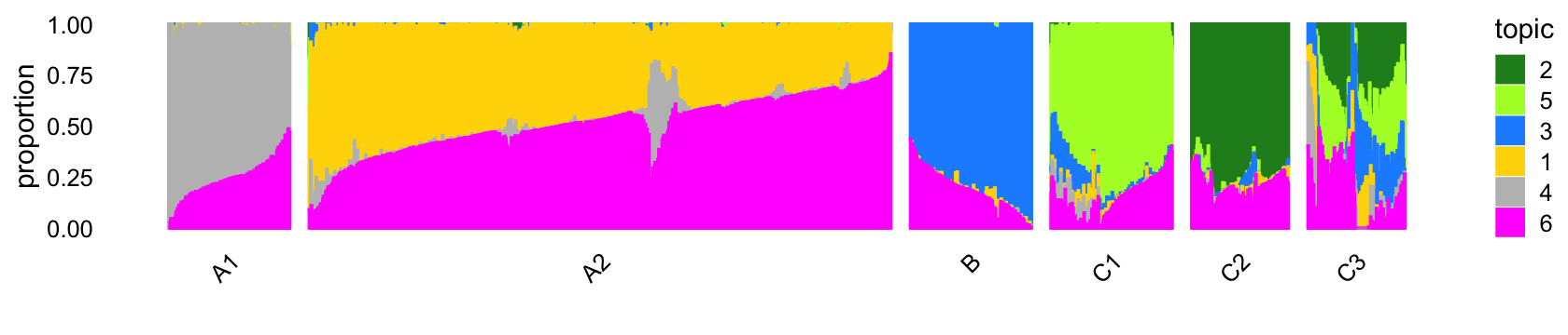
| Version | Author | Date |
|---|---|---|
| eac2d23 | Peter Carbonetto | 2020-08-25 |
| 2d156b8 | Peter Carbonetto | 2020-08-25 |
| abb846e | Peter Carbonetto | 2020-08-25 |
| f53c86c | Peter Carbonetto | 2020-08-24 |
| 13ee038 | Peter Carbonetto | 2020-08-23 |
| 97d7e86 | Peter Carbonetto | 2020-08-23 |
| 59777e7 | Peter Carbonetto | 2020-08-22 |
| c87ddf8 | Peter Carbonetto | 2020-08-22 |
| 7900d17 | Peter Carbonetto | 2020-08-22 |
| fbb0697 | Peter Carbonetto | 2020-08-21 |
| 216027a | Peter Carbonetto | 2020-08-21 |
Out of the 6 topics, 4 of them (\(k = 2, 3, 4, 5\)) align closely with the clusters (labeled A1, B, C1, C2). And, indeed, they align closely with their inclusion in the individual FACS-purified data sets:
pdat <- as.data.frame(with(samples_purified,table(celltype,cluster)))
ggplot(pdat,aes(x = cluster,y = celltype,size = Freq)) +
  geom_point(color = "dodgerblue",na.rm = TRUE,show.legend = FALSE) +
  ylim(rev(levels(samples_purified$celltype))) +
  theme_cowplot(font_size = 10)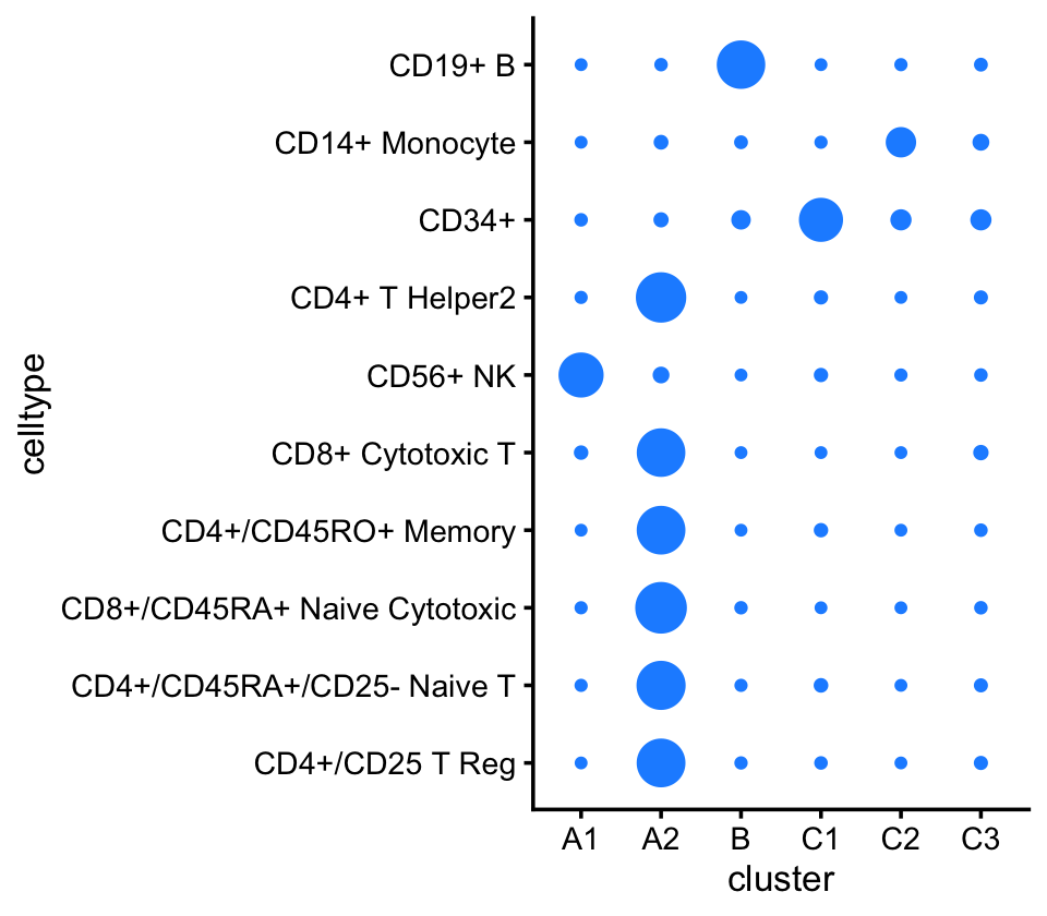
Based on the above results, we make a few observations:
Because they correspond very closely, subsequent analysis of topics 2, 3, 4 and 5 should yield similar results to analyzing the clusters A1, B, C1, C2 For example, cluster B corresponds almost perfectly to the B-cell data set. The largest cluster, cluster A2, is mostly comprised of the T-cell data sets.
Cluster A2—see also the PCA plot above—is an example where analyzing the most prevalent topics (\(k = 1, 6\)) will yield different results than analyzing clusters within cluster A1 as any additional clustering of the data will be necessarily arbitrary (see the PCA plot above).
Many samples labeled as “CD34+” are not assigned to the CD34+ cluster (C1). This is probably due to the fact that this population was much less pure (45%) than the others.
Cluster C3 is a heterogeneous cluster with a relatively small number of samples (790) that could potentially contain additional clusters of biological relevance, but will likely be more challenging to analyze and interpret than the other clusters, so we do not this investigate further.
In summary, a cluster-based analysis and topic-based analysis should yield mostly similar results, except for the analysis of cluster A2, which should benefit from a topic-based analysis (specifically, analysis of topics 1 and 6).
Unsorted 68k PBMC data
Next, we turn to the 68k data set.
load("../data/pbmc_68k.RData")
samples_68k <- samples
rm(samples,genes,counts)
Load the \(k = 6\) Poisson NMF model fit, and compute PCs from the topic proportions.
fit_68k <- readRDS("../output/pbmc-68k/rds/fit-pbmc-68k-scd-ex-k=6.rds")$fit
fit <- poisson2multinom(fit_68k)
pca <- prcomp(fit$L)$x
In this case, we find least three distinct clusters in the projection onto PCs 3 and 4. We label these clusters “A”, “B” and “C”, as above, noting that this labeling does not imply a connection with the purified PBMC clusters above.
n <- nrow(pca)
x <- rep("A",n)
pc3 <- pca[,"PC3"]
pc4 <- pca[,"PC4"]
x[pc4 < -0.13 | pc3/1.9 - 0.17 > pc4] <- "B"
x[pc4 < -0.75] <- "C"
samples_68k$cluster <- x
p5 <- pca_plot_with_labels(fit_68k,c("PC3","PC4"),x) +
      labs(fill = "cluster")
print(p5)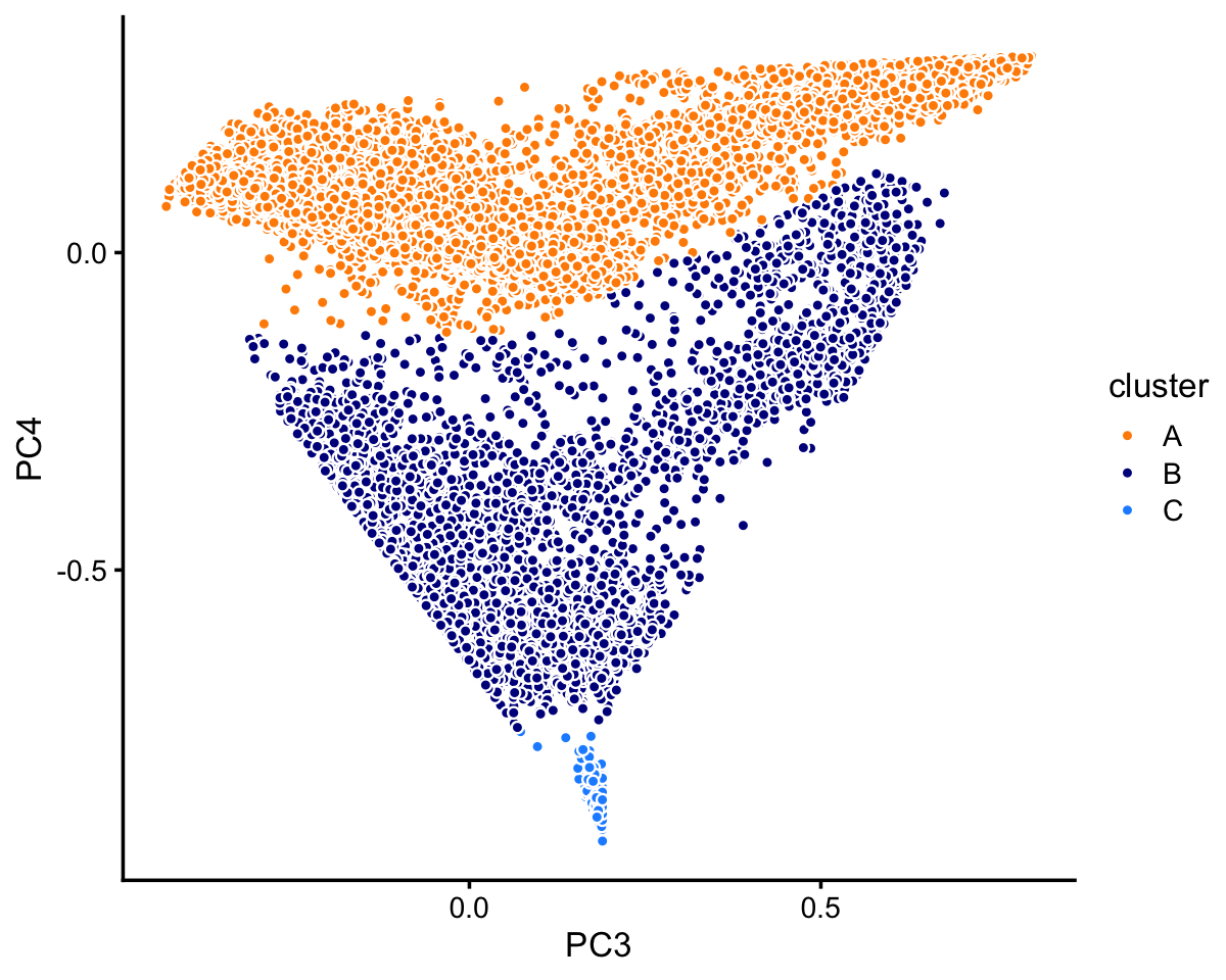
The vast majority of the cells are in cluster A.
table(samples_68k$cluster)
#
#     A     B     C
# 63408  5006   165
Looking more closely at the top two PCs in cluster B, we identify two large clusters, with the remaining samples assigned to the “B3” subset.
rows <- which(samples_68k$cluster == "B")
fit  <- select(poisson2multinom(fit_68k),loadings = rows)
pca  <- prcomp(fit$L)$x
n    <- nrow(pca)
x    <- rep("B3",n)
pc1  <- pca[,"PC1"]
x[pc1 > -0.05] <- "B1"
x[pc1 < -0.3] <- "B2"
samples_68k[rows,"cluster"] <- x
p6 <- pca_plot_with_labels(fit,c("PC1","PC2"),x) +
      labs(fill = "cluster")
print(p6)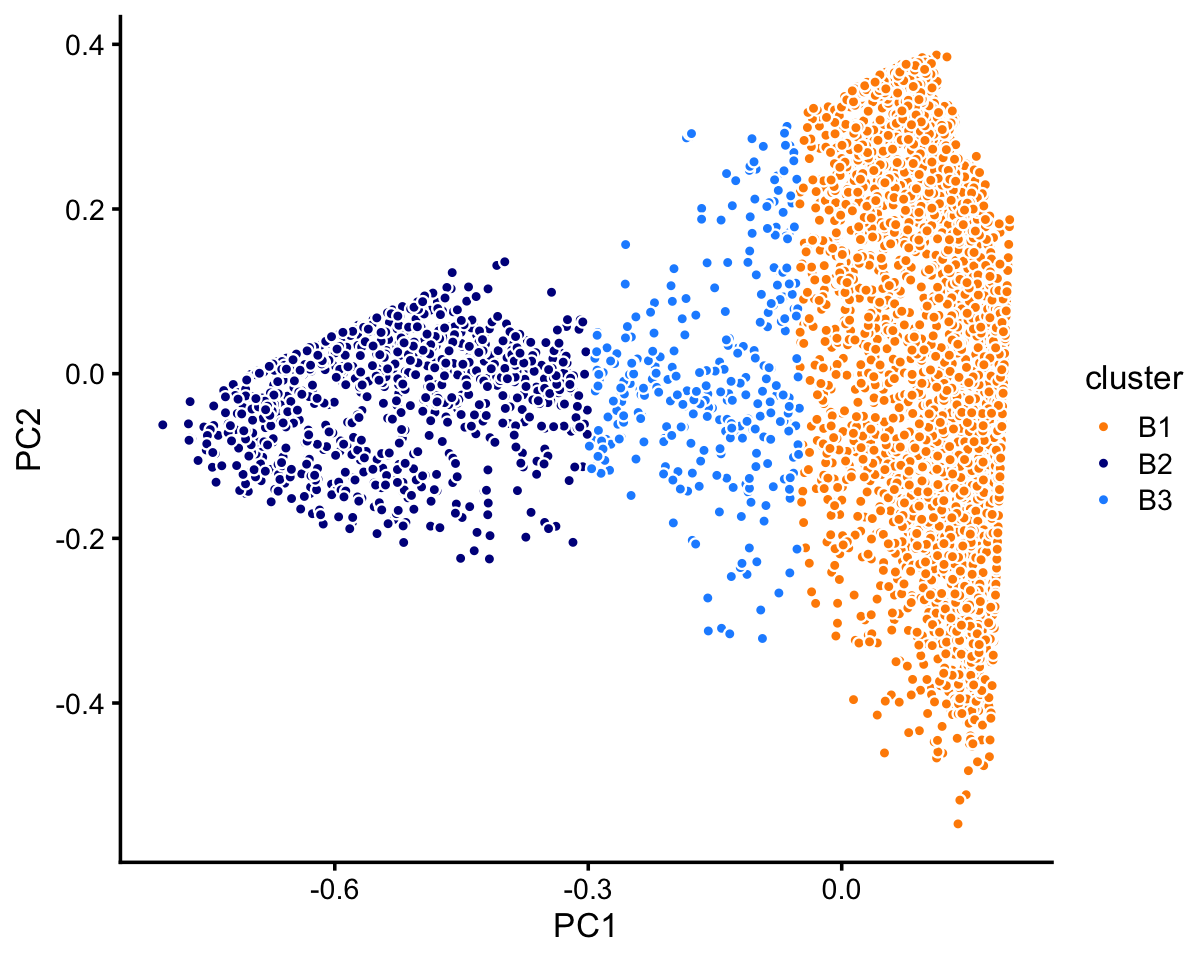
TO DO: Add text here.
rows <- which(samples_68k$cluster == "B1")
fit  <- select(poisson2multinom(fit_68k),loadings = rows)
pca  <- prcomp(fit$L)$x
n    <- nrow(pca)
x    <- rep("B1c",n)
pc1  <- pca[,"PC1"]
pc2  <- pca[,"PC2"]
x[pc2 > -0.02 & pc1 > -0.25] <- "B1a"
x[pc1 > 0.1 & pc2 < 0.05 & pc2 > -0.225] <- "B1b"
samples_68k[rows,"cluster"] <- x
p7 <- pca_plot_with_labels(fit,c("PC1","PC2"),x) +
      labs(fill = "cluster")
print(p7)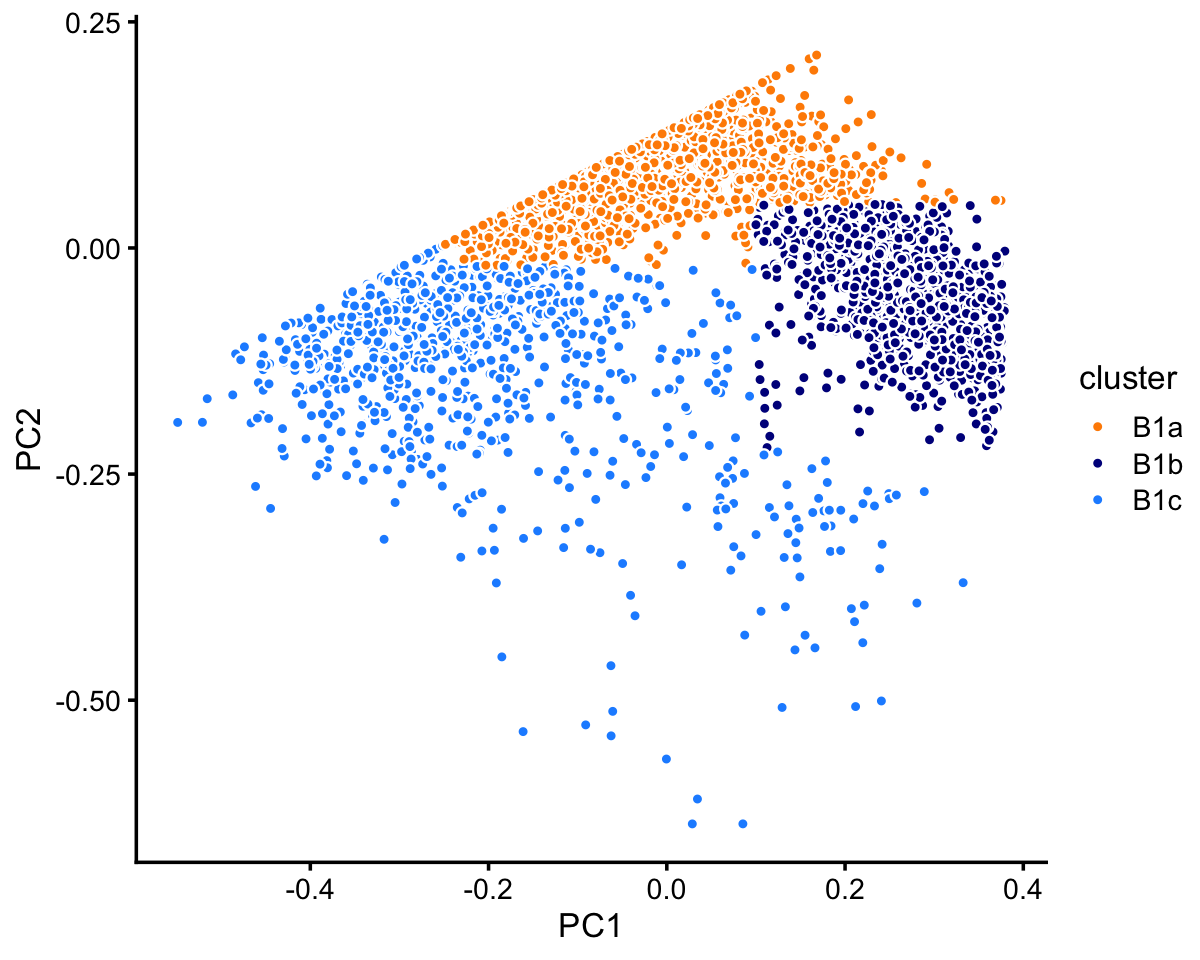
Cluster A subdivides fairly neatly into two large clusters, A1 and A2.
rows <- which(samples_68k$cluster == "A")
fit  <- select(poisson2multinom(fit_68k),loadings = rows)
pca  <- prcomp(fit$L)$x
n    <- nrow(pca)
x    <- rep("A3",n)
pc2  <- pca[,"PC2"]
pc3  <- pca[,"PC3"]
x[2.5*pc3 < 0.3 - pc2] <- "A1"
x[pc3 > 0.8 - pc2] <- "A2"
samples_68k[rows,"cluster"] <- x
p7 <- pca_plot_with_labels(fit,c("PC2","PC3"),x) +
      labs(fill = "cluster")
print(p7)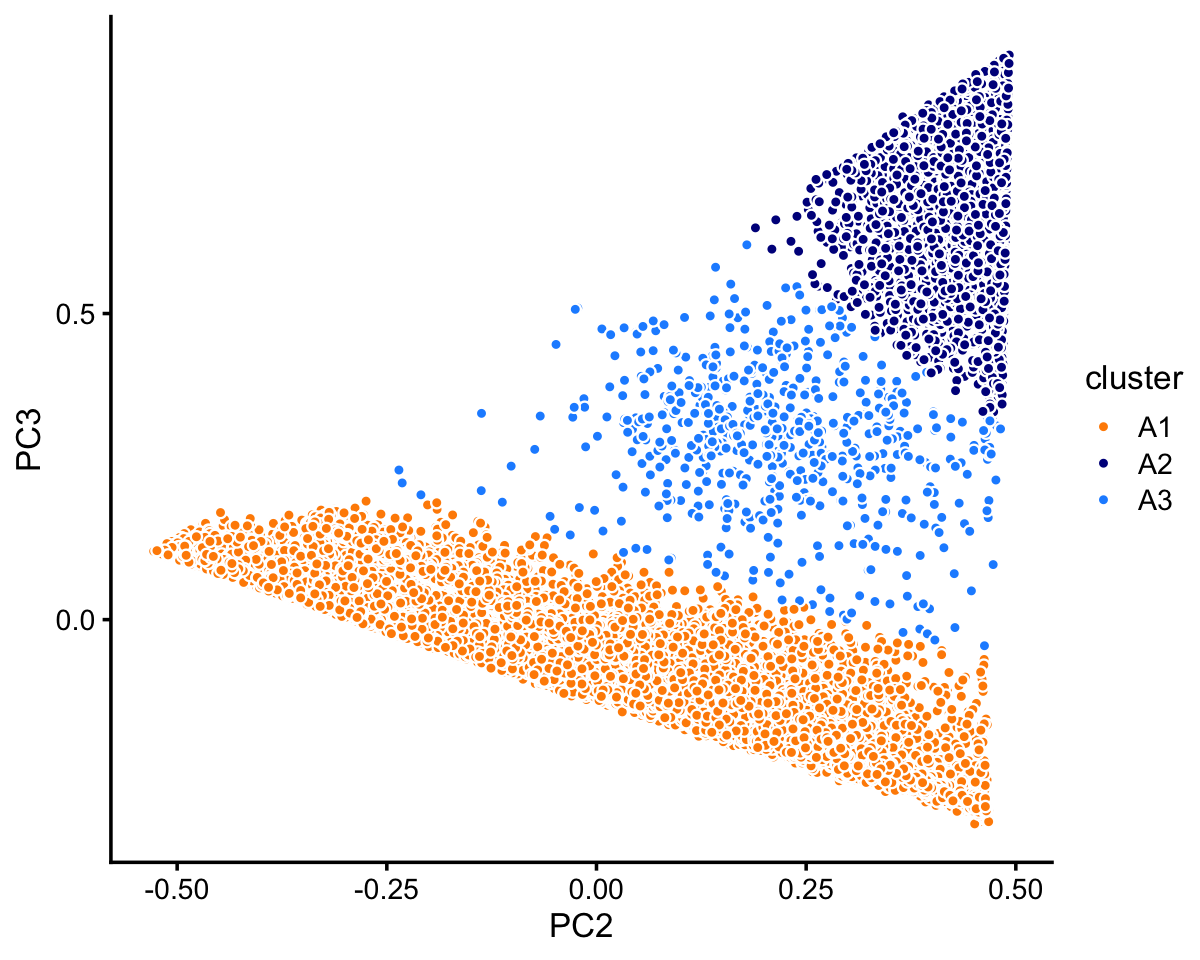
Within cluster A, the vast majority of the samples are assigned to the A1 subcluster:
table(x)
# x
#    A1    A2    A3
# 59260  3555   593
In summary, we have subdivided these data into 7 clusters:
samples_68k$cluster <- factor(samples_68k$cluster)
table(samples_68k$cluster)
#
#    A1    A2    A3   B1a   B1b   B1c    B2    B3     C
# 59260  3555   593  2115   947   807   819   318   165
The wide range in the sizes of these clusters is notable; the smallest cluster (C) is less than 1% the size of the largest (A1). By contrast, community detection methods such as the Louvain algorithm often have difficulty identifying very small clusters.
TO DO: Add text here.
set.seed(1)
pbmc_68k_topic_colors <- c("yellow","lightskyblue","salmon",
                           "firebrick","royalblue","olivedrab")
pbmc_68k_topics <- c(2,5,1,3,4,6)
rows <- sort(c(sample(which(samples_68k$cluster == "A1"),1200),
               sample(which(samples_68k$cluster == "A2"),500),
               sample(which(samples_68k$cluster == "A3"),300),
               sample(which(samples_68k$cluster == "B1a"),500),
               sample(which(samples_68k$cluster == "B1b"),300),
               sample(which(samples_68k$cluster == "B1c"),300),
               sample(which(samples_68k$cluster == "B2"),300),
               which(samples_68k$cluster == "B3"),
               which(samples_68k$cluster == "C")))
p8 <- structure_plot(select(poisson2multinom(fit_68k),loadings = rows),
                     grouping = samples_68k[rows,"cluster"],
                     topics = pbmc_68k_topics,
                     colors = pbmc_68k_topic_colors[pbmc_68k_topics],
                     perplexity = c(100,100,50,100,80,80,80,80,50),
                     n = Inf,gap = 32,num_threads = 4,verbose = FALSE)
print(p8)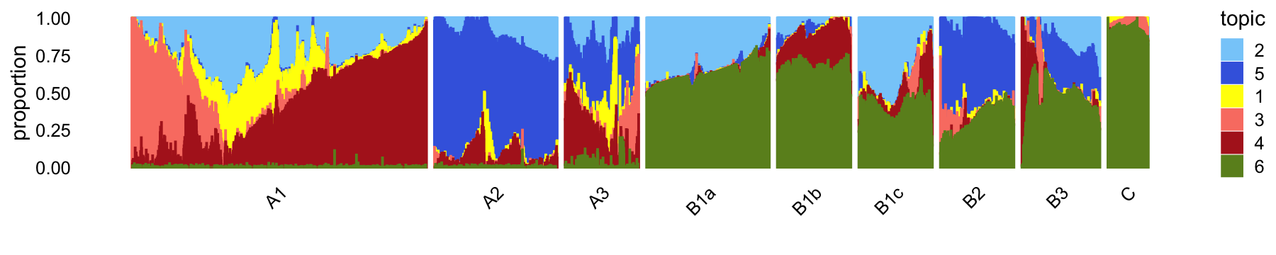
Comparison to Zheng et al (2017) cell-type labeling:
pdat <- as.data.frame(with(samples_68k,table(celltype,cluster)))
ggplot(pdat,aes(x = cluster,y = celltype,size = Freq)) +
  geom_point(color = "dodgerblue",na.rm = TRUE,show.legend = FALSE) +
  ylim(rev(levels(samples_purified$celltype))) +
  theme_cowplot(font_size = 10)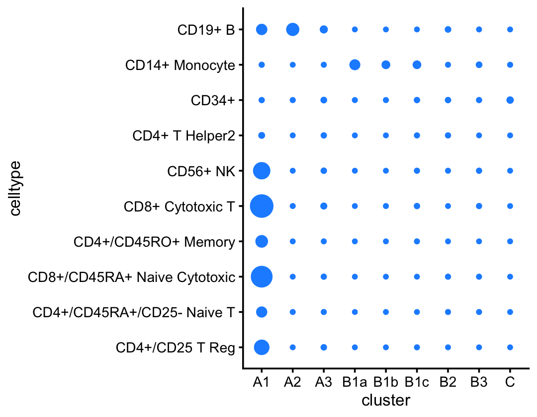
sessionInfo()
# R version 3.6.2 (2019-12-12)
# Platform: x86_64-apple-darwin15.6.0 (64-bit)
# Running under: macOS Catalina 10.15.5
#
# Matrix products: default
# BLAS:   /Library/Frameworks/R.framework/Versions/3.6/Resources/lib/libRblas.0.dylib
# LAPACK: /Library/Frameworks/R.framework/Versions/3.6/Resources/lib/libRlapack.dylib
#
# locale:
# [1] en_US.UTF-8/en_US.UTF-8/en_US.UTF-8/C/en_US.UTF-8/en_US.UTF-8
#
# attached base packages:
# [1] stats     graphics  grDevices utils     datasets  methods   base
#
# other attached packages:
# [1] cowplot_1.0.0      ggplot2_3.3.0      fastTopics_0.3-165 dplyr_0.8.3
#
# loaded via a namespace (and not attached):
#  [1] ggrepel_0.9.0        Rcpp_1.0.5           lattice_0.20-38
#  [4] tidyr_1.0.0          prettyunits_1.1.1    assertthat_0.2.1
#  [7] zeallot_0.1.0        rprojroot_1.3-2      digest_0.6.23
# [10] R6_2.4.1             backports_1.1.5      MatrixModels_0.4-1
# [13] evaluate_0.14        coda_0.19-3          httr_1.4.1
# [16] pillar_1.4.3         rlang_0.4.5          progress_1.2.2
# [19] lazyeval_0.2.2       data.table_1.12.8    irlba_2.3.3
# [22] SparseM_1.78         whisker_0.4          Matrix_1.2-18
# [25] rmarkdown_2.3        labeling_0.3         Rtsne_0.15
# [28] stringr_1.4.0        htmlwidgets_1.5.1    munsell_0.5.0
# [31] compiler_3.6.2       httpuv_1.5.2         xfun_0.11
# [34] pkgconfig_2.0.3      mcmc_0.9-6           htmltools_0.4.0
# [37] tidyselect_0.2.5     tibble_2.1.3         workflowr_1.6.2.9000
# [40] quadprog_1.5-8       viridisLite_0.3.0    crayon_1.3.4
# [43] withr_2.1.2          later_1.0.0          MASS_7.3-51.4
# [46] grid_3.6.2           jsonlite_1.6         gtable_0.3.0
# [49] lifecycle_0.1.0      git2r_0.26.1         magrittr_1.5
# [52] scales_1.1.0         RcppParallel_5.0.2   stringi_1.4.3
# [55] farver_2.0.1         fs_1.3.1             promises_1.1.0
# [58] vctrs_0.2.1          tools_3.6.2          glue_1.3.1
# [61] purrr_0.3.3          hms_0.5.2            yaml_2.2.0
# [64] colorspace_1.4-1     plotly_4.9.2         knitr_1.26
# [67] quantreg_5.54        MCMCpack_1.4-5