Visualize and interpret droplet and pulse-seq topics
Peter Carbonetto
Last updated: 2020-08-20
Checks: 7 0
Knit directory: single-cell-topics/analysis/
This reproducible R Markdown analysis was created with workflowr (version 1.6.2.9000). The Checks tab describes the reproducibility checks that were applied when the results were created. The Past versions tab lists the development history.
Great! Since the R Markdown file has been committed to the Git repository, you know the exact version of the code that produced these results.
Great job! The global environment was empty. Objects defined in the global environment can affect the analysis in your R Markdown file in unknown ways. For reproduciblity it’s best to always run the code in an empty environment.
The command set.seed(1) was run prior to running the code in the R Markdown file. Setting a seed ensures that any results that rely on randomness, e.g. subsampling or permutations, are reproducible.
Great job! Recording the operating system, R version, and package versions is critical for reproducibility.
Nice! There were no cached chunks for this analysis, so you can be confident that you successfully produced the results during this run.
Great job! Using relative paths to the files within your workflowr project makes it easier to run your code on other machines.
Great! You are using Git for version control. Tracking code development and connecting the code version to the results is critical for reproducibility.
The results in this page were generated with repository version 961570e. See the Past versions tab to see a history of the changes made to the R Markdown and HTML files.
Note that you need to be careful to ensure that all relevant files for the analysis have been committed to Git prior to generating the results (you can use wflow_publish or wflow_git_commit). workflowr only checks the R Markdown file, but you know if there are other scripts or data files that it depends on. Below is the status of the Git repository when the results were generated:
Ignored files:
    Ignored:    data/droplet.RData
    Ignored:    data/pbmc_68k.RData
    Ignored:    data/pbmc_purified.RData
    Ignored:    data/pulseseq.RData
    Ignored:    output/droplet/fits-droplet.RData
    Ignored:    output/droplet/rds/
    Ignored:    output/pbmc-68k/fits-pbmc-68k.RData
    Ignored:    output/pbmc-68k/rds/
    Ignored:    output/pbmc-purified/fits-pbmc-purified.RData
    Ignored:    output/pbmc-purified/rds/
    Ignored:    output/pulseseq/fits-pulseseq.RData
    Ignored:    output/pulseseq/rds/
Note that any generated files, e.g. HTML, png, CSS, etc., are not included in this status report because it is ok for generated content to have uncommitted changes.
These are the previous versions of the repository in which changes were made to the R Markdown (analysis/plots_tracheal_epithelium.Rmd) and HTML (docs/plots_tracheal_epithelium.html) files. If you’ve configured a remote Git repository (see ?wflow_git_remote), click on the hyperlinks in the table below to view the files as they were in that past version.
| File | Version | Author | Date | Message |
|---|---|---|---|---|
| Rmd | 961570e | Peter Carbonetto | 2020-08-20 | wflow_publish(“plots_tracheal_epithelium.Rmd”) |
| html | b17bfa4 | Peter Carbonetto | 2020-08-19 | Added pulseseq PCA plots to plots_tracheal_epithelium analysis. |
| Rmd | 76dc0c6 | Peter Carbonetto | 2020-08-19 | wflow_publish(“plots_tracheal_epithelium.Rmd”) |
| Rmd | c70612f | Peter Carbonetto | 2020-08-19 | Revised structure plot settings for abundant droplet samples in plots_tracheal_epithelium. |
| html | adda33f | Peter Carbonetto | 2020-08-19 | Fixed another structure plot in plots_tracheal_epithelium analysis. |
| Rmd | 29a9258 | Peter Carbonetto | 2020-08-19 | wflow_publish(“plots_tracheal_epithelium.Rmd”) |
| html | 0a16b60 | Peter Carbonetto | 2020-08-19 | Fixed structure plot in plots_tracheal_epithelium analysis. |
| Rmd | 3a7bd74 | Peter Carbonetto | 2020-08-19 | wflow_publish(“plots_tracheal_epithelium.Rmd”) |
| html | f4bdf19 | Peter Carbonetto | 2020-08-19 | Added explanatory text and improved PC-based manual clustering of |
| Rmd | c7b77ee | Peter Carbonetto | 2020-08-19 | wflow_publish(“plots_tracheal_epithelium.Rmd”) |
| Rmd | 70a4a60 | Peter Carbonetto | 2020-08-19 | Added note to plots_tracheal_epithelium.Rmd. |
| html | fb21b3b | Peter Carbonetto | 2020-08-19 | Added very initial Structure plots to plots_tracheal_epithelium analysis. |
| Rmd | d35cb03 | Peter Carbonetto | 2020-08-19 | wflow_publish(“plots_tracheal_epithelium.Rmd”) |
| html | 368a74a | Peter Carbonetto | 2020-08-19 | Added some text to plots_tracheal_epithelium analysis. |
| Rmd | 223406b | Peter Carbonetto | 2020-08-19 | wflow_publish(“plots_tracheal_epithelium.Rmd”) |
| html | aca46cc | Peter Carbonetto | 2020-08-19 | Added manual clustering of droplet samples based on PCs. |
| Rmd | 38f811b | Peter Carbonetto | 2020-08-19 | wflow_publish(“plots_tracheal_epithelium.Rmd”) |
| Rmd | 343747e | Peter Carbonetto | 2020-08-19 | Small edit to figure dimensions. |
| html | 5a35bbd | Peter Carbonetto | 2020-08-19 | Added labeled PCA plot; adjusted plot dimensions in |
| Rmd | fb91075 | Peter Carbonetto | 2020-08-19 | wflow_publish(“plots_tracheal_epithelium.Rmd”) |
| html | 8b9b528 | Peter Carbonetto | 2020-08-19 | Added more PCA plots to plots_tracheal_epithelium analysis. |
| Rmd | ee7cbf1 | Peter Carbonetto | 2020-08-19 | wflow_publish(“plots_tracheal_epithelium.Rmd”) |
| html | c517ea2 | Peter Carbonetto | 2020-08-18 | Small fix to one of the PCA plots in plots_tracheal_epithelium. |
| Rmd | 8f5c210 | Peter Carbonetto | 2020-08-18 | wflow_publish(“plots_tracheal_epithelium.Rmd”) |
| html | 01afbd2 | Peter Carbonetto | 2020-08-18 | Added some PC plots to the plots_tracheal_epithelium analysis. |
| Rmd | f1c7d02 | Peter Carbonetto | 2020-08-18 | wflow_publish(“plots_tracheal_epithelium.Rmd”) |
| html | 0a04fc1 | Peter Carbonetto | 2020-08-18 | Added abundance plots to plots_tracheal_epithelium analysis. |
| Rmd | f914f7e | Peter Carbonetto | 2020-08-18 | wflow_publish(“plots_tracheal_epithelium.Rmd”) |
| Rmd | 61917ad | Peter Carbonetto | 2020-08-18 | Working on new analysis, plots_tracheal_epithelium.Rmd. |
TO DO: Add introductory text here.
Load the packages used in the analysis below.
library(fastTopics)
library(dplyr)
library(ggplot2)
library(cowplot)
source("../code/plots.R")
Load the sample annotations. (The count data are no longer needed at this stage of the analysis.)
load("../data/droplet.RData")
samples_droplet <- samples
load("../data/pulseseq.RData")
samples_pulseseq <- samples
rm(samples,counts)
Load the \(k = 7\) Poisson NMF model fit for the droplet data, and the \(k = 11\) Poisson NMF fit for the pulse-seq data.
fit_droplet <- readRDS("../output/droplet/rds/fit-droplet-scd-ex-k=7.rds")$fit
fit_pulseseq <- readRDS("../output/pulseseq/rds/fit-pulseseq-scd-ex-k=11.rds")$fit
The Montoro et al (2018) article mentions that some epithelial cell types are abundant, whereas others are very rare. The topics in the droplet data reflect this:
p1 <- create_abundance_plot(fit_droplet)
print(p1)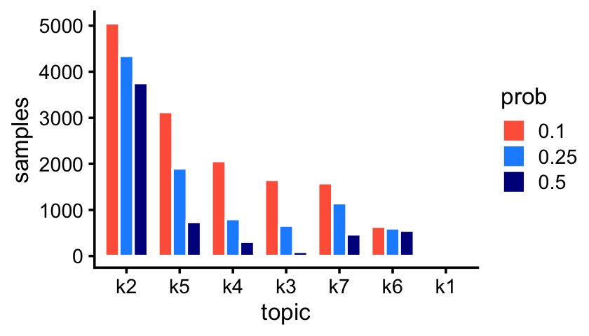
| Version | Author | Date |
|---|---|---|
| 0a04fc1 | Peter Carbonetto | 2020-08-18 |
The first topic—which is not visible in the bar chart—is indeed very rare; only 43 out of 7,193 samples have a greater than 10% contribution from this topic.
sum(poisson2multinom(fit_droplet)$L[,1] > 0.1)
# [1] 43
Likewise, we also pick up rare and abundant topics in the pulse-seq data:
p2 <- create_abundance_plot(fit_pulseseq)
print(p2)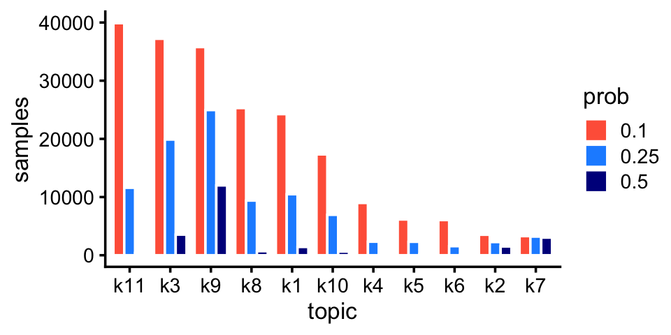
| Version | Author | Date |
|---|---|---|
| 0a04fc1 | Peter Carbonetto | 2020-08-18 |
In this next part of the analysis, we perform PCA on the estimated topic proportions to explore structure in the data as inferred by the topic model. Typically a nonlinear embedding method such as t-SNE or UMAP is used to visualize the structure, but the disadvantage such methods is that it can often be difficult to get the (many) tuning parameters right, and they are sometimes very slow for large data sets; by contrast, PCA has no tuning parameters.
These three scatterplots show the droplet samples (the topic proportions) projected onto 5 out of the 7 PCs. (PCs 3 and 7 do not reveal any additional structure, so are not shown here.)
p3 <- basic_pca_plot(fit_droplet,c("PC1","PC2"))
p4 <- basic_pca_plot(fit_droplet,c("PC4","PC5"))
p5 <- basic_pca_plot(fit_droplet,c("PC5","PC6"))
plot_grid(p3,p4,p5,nrow = 1)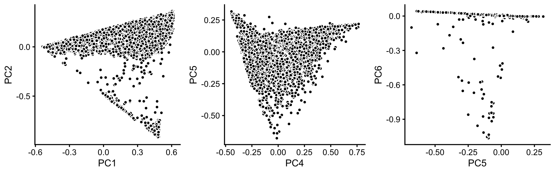
Distinct clusters show up in the PC1 vs. PC2 plot, as well as in the PC5 vs. PC6 plot, whereas the structure in PC4 vs. PC5 is very much continuously varying.
Let’s look more closely at the topics that show variation in the first two PCs:
p6 <- pca_plot(poisson2multinom(fit_droplet),pcs = 1:2,k = c(2,5,6),
               plot_grid_call = function (plots)
                 do.call(plot_grid,c(lapply(plots,
                   function (x) x + guides(fill = "none")),list(nrow = 1))))
print(p6)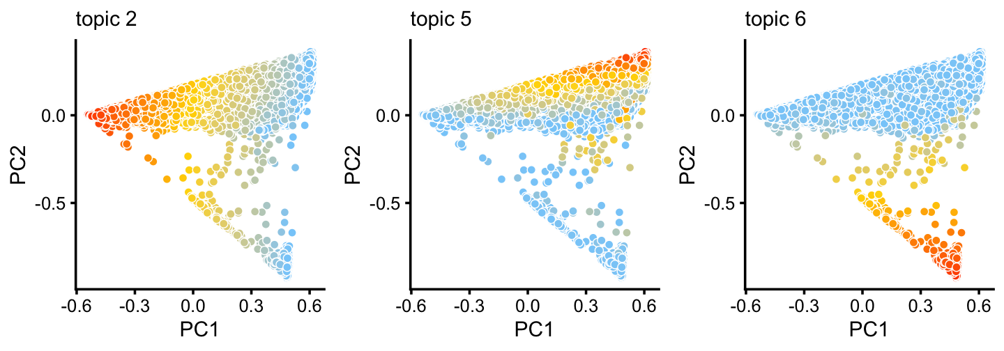
The bulk of the samples lie on a continuous gradient between topics 2 and 5. There is a smaller cluster at the bottom of this plot, with high contributions from topic 6.
Next, we look closely at PCs 4 and 5:
p7 <- pca_plot(poisson2multinom(fit_droplet),pcs = 4:5,k = c(3,4,5,7),
               plot_grid_call = function (plots)
                 do.call(plot_grid,c(lapply(plots,
                   function (x) x + guides(fill = "none")),list(nrow = 1))))
print(p7)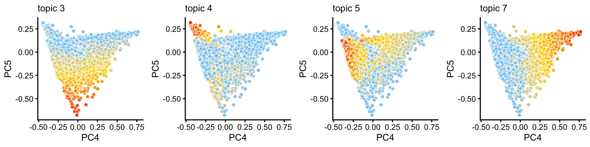
Along these PCs, we see that topics 3, 4, 5 and 7 exist in many combinations, with no apparent distinct populations.
Topic 1 captures a very small discrete population of cells:
p8 <- pca_plot(poisson2multinom(fit_droplet),pcs = 5:6,k = 1) +
        guides(fill = "none")
print(p8)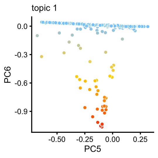
| Version | Author | Date |
|---|---|---|
| 8b9b528 | Peter Carbonetto | 2020-08-19 |
In summary, topics 1 and 6 pick up discrete “cell types”, whereas the other topics characterize more continuous variation in gene expression, perhaps cell types along a continuous trajectory of development. There are some other discrete clusters that seem to be composed of distinct combinations of topics that we will neeed to examine more closely.
As suggested by this analysis, we can easily delineate four clusters, the majority of which are included in cluster labeled c_1$. Here we construct this clustering by hand, using the PCs computed from the topic cproportions:
pca_droplet <- prcomp(poisson2multinom(fit_droplet)$L)$x
n    <- nrow(pca_droplet)
x    <- rep("c0",n)
pc1  <- pca_droplet[,"PC1"]
pc2  <- pca_droplet[,"PC2"]
pc6  <- pca_droplet[,"PC6"]
x[pc2 > -0.1]  <- "c1"
x[pc6 < -0.04] <- "c2"
x[(pc1 - 0)^2 + (pc2 + 0.75)^2 < 0.09]  <- "c3"
x[(pc1 - 0.5)^2 + (pc2 + 0.9)^2 < 0.04] <- "c4"
samples_droplet$cluster <- factor(x)
print(table(samples_droplet$cluster))
#
#   c0   c1   c2   c3   c4
#   73 6533   50  162  375
Indeed, the vast majority of the cells are in the \(c_1\) cluster.
These next few scatterplots show the same PCs as before, with the samples labeled according to their assignment to these clusters:
droplet_cluster_colors <- c("gray","darkblue","gold","yellowgreen","firebrick")
p9 <- pca_plot_with_labels(fit_droplet,c("PC1","PC2"),samples_droplet$cluster,
                           droplet_cluster_colors) + labs(fill = "cluster")
p10 <- pca_plot_with_labels(fit_droplet,c("PC4","PC5"),samples_droplet$cluster,
                            droplet_cluster_colors) + labs(fill = "cluster")
p11 <- pca_plot_with_labels(fit_droplet,c("PC5","PC6"),samples_droplet$cluster,
                            droplet_cluster_colors) + labs(fill = "cluster")
plot_grid(p9,p10,p11)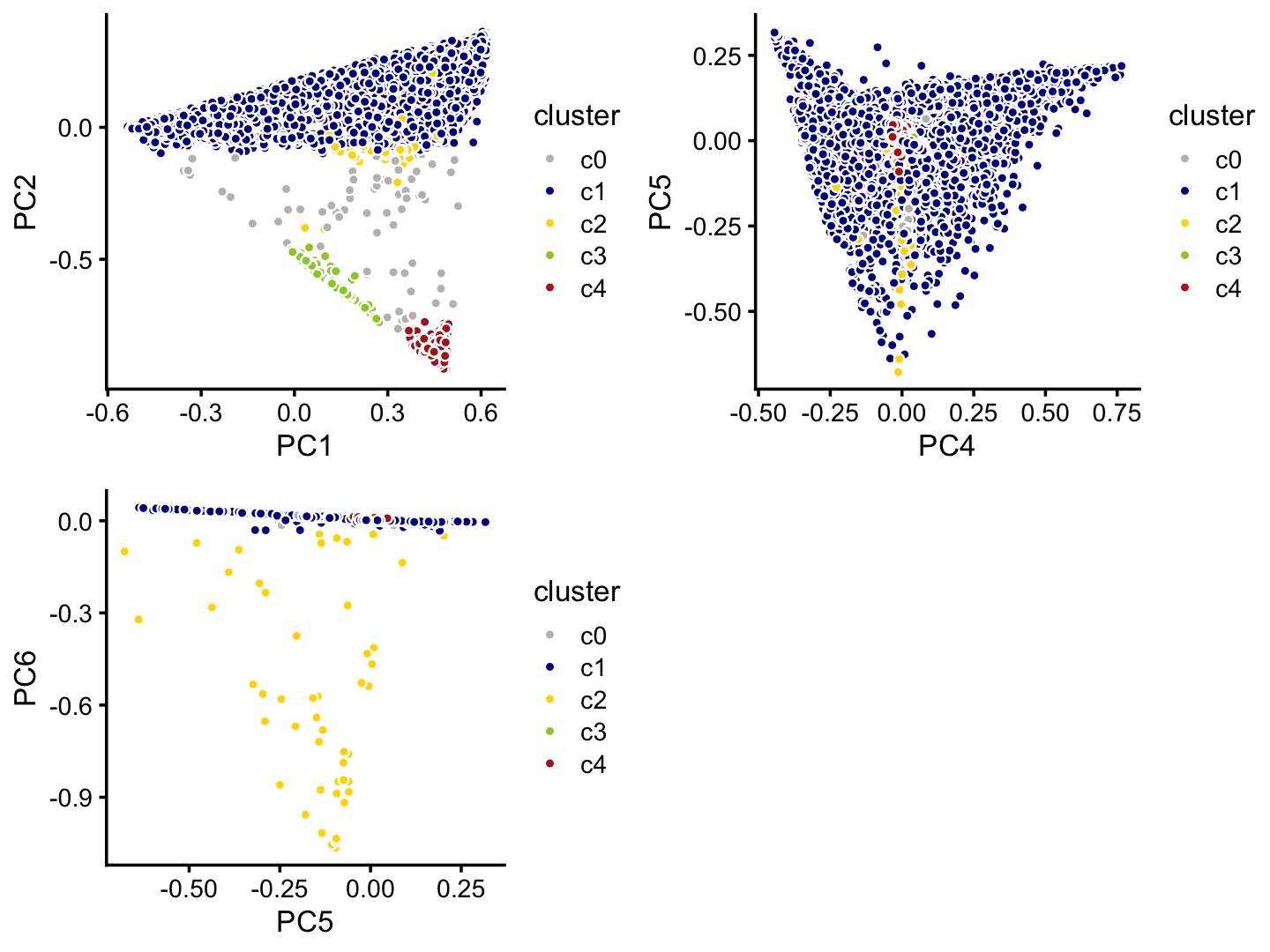
In the following, we will treat the more abundant clusters, \(c_1\) and \(c_4\), separately from the rest of the samples.
TO DO: Add text here.
p12 <- pca_plot(poisson2multinom(fit_pulseseq),pcs = 3:4,k = 7)
p13 <- pca_plot(poisson2multinom(fit_pulseseq),pcs = 5:6,k = 2)
plot_grid(p12,p13)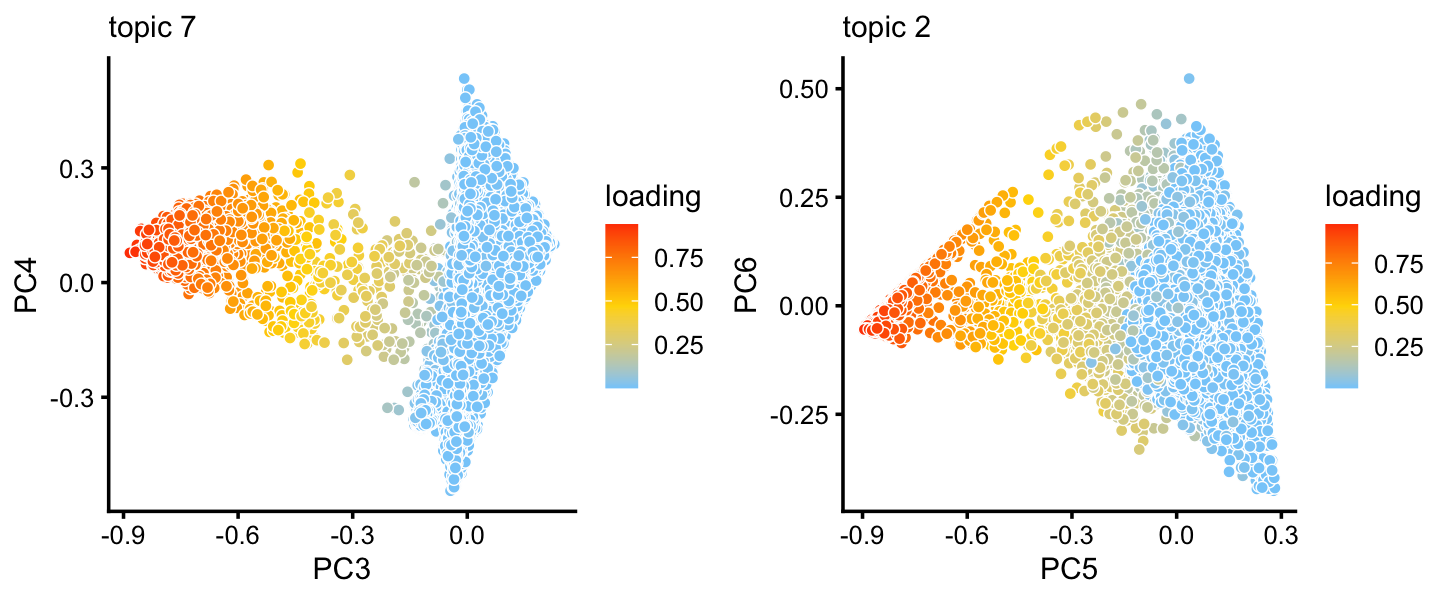
| Version | Author | Date |
|---|---|---|
| b17bfa4 | Peter Carbonetto | 2020-08-19 |
TO DO: Add text here.
droplet_topic_colors <- c("gold","royalblue","turquoise","greenyellow",
                          "forestgreen","firebrick","olivedrab")
names(droplet_topic_colors) <- paste0("k",1:7)
topics <- c("k1","k3","k4","k5","k7","k2","k6")
set.seed(1)
fit_droplet_rare <- select(poisson2multinom(fit_droplet),
                           loadings = which(samples_droplet$cluster != "c1" &
                                            samples_droplet$cluster != "c4"))
p12 <- structure_plot(fit_droplet_rare,verbose = FALSE,perplexity = 50,
                      topics = topics,
                      colors = droplet_topic_colors[topics])
print(p12)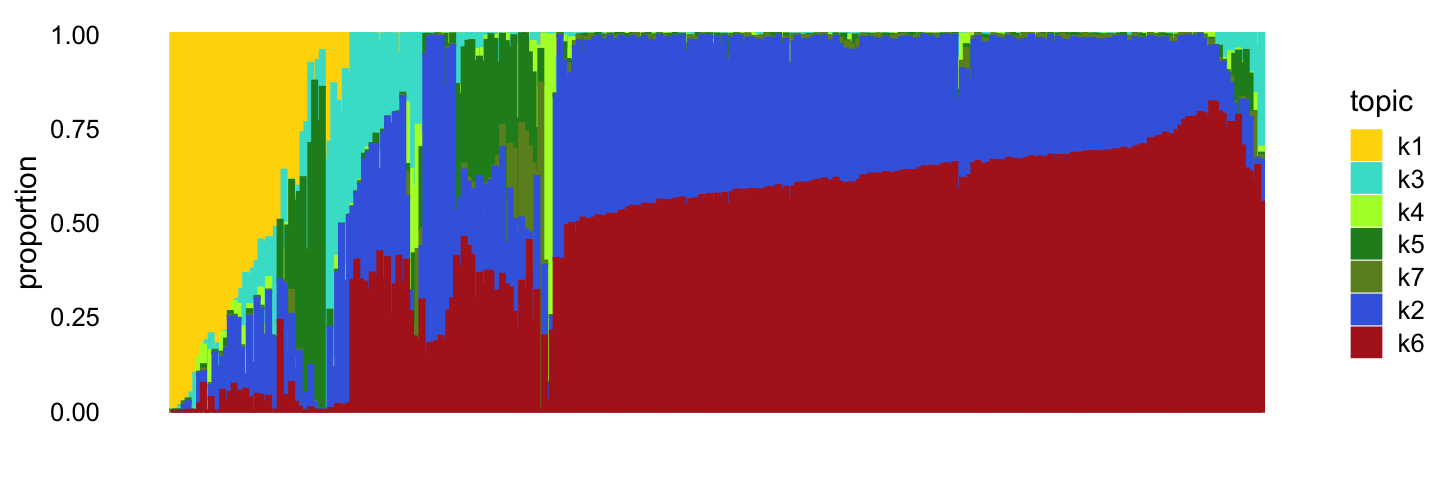
TO DO: Add text here.
topics <- c("k1","k3","k4","k7","k5","k2","k6")
set.seed(1)
fit_droplet_abundant <-
  select(poisson2multinom(fit_droplet),
                          loadings = which(samples_droplet$cluster == "c1" |
                                           samples_droplet$cluster == "c4"))
p13 <- structure_plot(fit_droplet_abundant,n = 2000,perplexity = 50,
                      verbose = FALSE,topics = topics,
                      colors = droplet_topic_colors[topics],
                      scaling = c(1,1,1,1,2,1,1))
print(p13)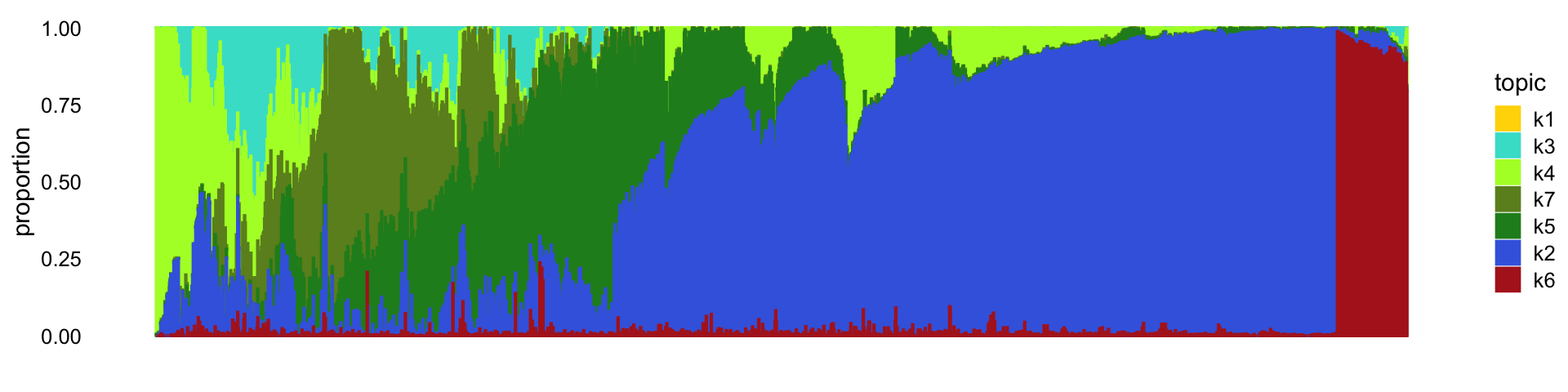
temp <- select(poisson2multinom(fit_droplet),
               loadings = which(samples_droplet$tissue == "Ionocyte"))
structure_plot(temp,rows = order(temp$L[,3]),
                      topics = topic_ordering,
                      colors = droplet_topic_colors[topic_ordering])
temp2 <- select(poisson2multinom(fit_droplet),
                loadings = which(samples_droplet$tissue == "Tuft"))
structure_plot(temp2,perplexity = 30,
               topics = topic_ordering,
               colors = droplet_topic_colors[topic_ordering])
temp3 <- select(poisson2multinom(fit_droplet),
                loadings = which(samples_droplet$tissue == "Neuroendocrine"))
structure_plot(temp3,perplexity = 30,
               topics = topic_ordering,
               colors = droplet_topic_colors[topic_ordering])
It is helpful to compare these results with clustering reported in the Montoro et al (2018) paper. To make this comparison, we layer the 7 clusters on top of these PCs:
droplet_celltype_colors <-
  c("royalblue",      # Basal
    "firebrick",      # Ciliated
    "forestgreen",    # Club
    "gold",           # Goblet
    "darkmagenta",    # Ionocyte
    "darkorange",     # Neuroendocrine
    "lightsteelblue") # Tuft
p9 <- pca_plot_with_labels(fit_droplet,c("PC1","PC2"),samples_droplet$tissue,
                           droplet_celltype_colors) + labs(fill = "celltype")
p10 <- pca_plot_with_labels(fit_droplet,c("PC4","PC5"),samples_droplet$tissue,
                            droplet_celltype_colors) + labs(fill = "celltype")
p11 <- pca_plot_with_labels(fit_droplet,c("PC5","PC6"),samples_droplet$tissue,
                            droplet_celltype_colors) + labs(fill = "celltype")
plot_grid(p9,p10,p11)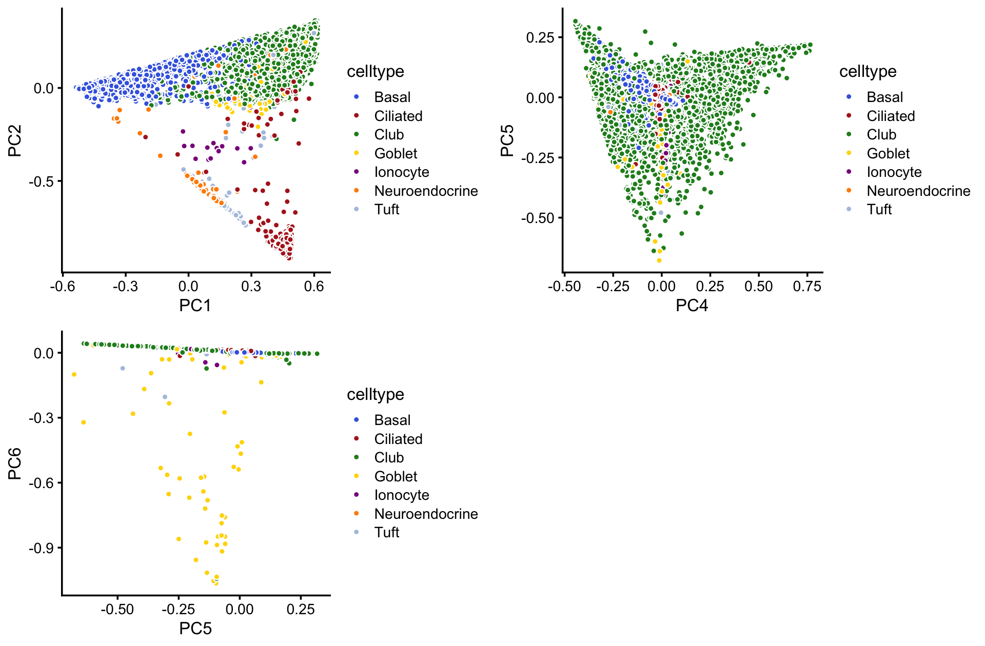
TO DO: Add Structure plot9s) to compare Montoro et al (2018) clustering.
And likewise in the pulse-seq data:
p5 <- basic_pca_plot(fit_pulseseq,c("PC3","PC4"))
p6 <- basic_pca_plot(fit_pulseseq,c("PC5","PC6"))
plot_grid(p5,p6)
ggplot(cbind(pca$x,data.frame(k2 = fit$L[,2])),
aes(x = PC1,y = PC2,fill = k2)) +
geom_point(shape = 21,color = "white",size = 2) +
scale_fill_gradient2(low = "deepskyblue",mid = "gold",high = "orangered",
midpoint = 0.5) +
theme_cowplot(font_size = 12)
ggplot(cbind(pca$x,data.frame(k5 = fit$L[,5])),
aes(x = PC1,y = PC2,fill = k5)) +
geom_point(shape = 21,color = "white",size = 2) +
scale_fill_gradient2(low = "deepskyblue",mid = "gold",high = "orangered",
midpoint = 0.5) +
theme_cowplot(font_size = 12)
ggplot(cbind(pca$x,data.frame(k6 = fit$L[,6])),
aes(x = PC1,y = PC2,fill = k6)) +
geom_point(shape = 21,color = "white",size = 2) +
scale_fill_gradient2(low = "deepskyblue",mid = "gold",high = "orangered",
midpoint = 0.5) +
theme_cowplot(font_size = 12)
ggplot(cbind(pca$x,data.frame(k1 = fit$L[,1])),
aes(x = PC5,y = PC6,fill = k1)) +
geom_point(shape = 21,color = "white",size = 2) +
scale_fill_gradient2(low = "deepskyblue",mid = "gold",high = "orangered",
midpoint = 0.5) +
theme_cowplot(font_size = 12)ggplot(cbind(pca$x,data.frame(k3 = fit$L[,3])),
aes(x = PC1,y = PC2,fill = k3)) +
geom_point(shape = 21,color = "white",size = 2) +
scale_fill_gradient2(low = "deepskyblue",mid = "gold",high = "orangered",
midpoint = 0.5) +
theme_cowplot(font_size = 12)
ggplot(cbind(pca$x,data.frame(k4 = fit$L[,4])),
aes(x = PC1,y = PC2,fill = k4)) +
geom_point(shape = 21,color = "white",size = 2) +
scale_fill_gradient2(low = "deepskyblue",mid = "gold",high = "orangered",
midpoint = 0.5) +
theme_cowplot(font_size = 12)ggplot(cbind(samples_droplet,pca$x),aes(x = PC1,y = PC2,fill = tissue)) +
geom_point(shape = 21,color = "white",size = 2) +
scale_fill_manual(values = clrs) +
theme_cowplot(font_size = 12)
ggplot(cbind(samples_droplet,pca$x),aes(x = PC5,y = PC6,fill = tissue)) +
geom_point(shape = 21,color = "white",,size = 2) +
scale_fill_manual(values = clrs) +
theme_cowplot(font_size = 12)clrs <- c("royalblue", # basal
"firebrick", # ciliated
"forestgreen", # club
"gold", # goblet
"darkmagenta", # ionocyte
"darkorange", # neuroendocrine
"tomato", # proliferating
"darkgray") # tuft
ggplot(cbind(samples_droplet,pca$x),aes(x = PC1,y = PC2,fill = tissue)) +
  geom_point(shape = 21,color = "white",size = 2) +
  scale_fill_manual(values = clrs) +
  theme_cowplot(font_size = 12)
ggplot(cbind(samples_droplet,pca$x),aes(x = PC5,y = PC6,fill = tissue)) +
  geom_point(shape = 21,color = "white",,size = 2) +
  scale_fill_manual(values = clrs) +
  theme_cowplot(font_size = 12)
sessionInfo()
# R version 3.6.2 (2019-12-12)
# Platform: x86_64-apple-darwin15.6.0 (64-bit)
# Running under: macOS Catalina 10.15.5
#
# Matrix products: default
# BLAS:   /Library/Frameworks/R.framework/Versions/3.6/Resources/lib/libRblas.0.dylib
# LAPACK: /Library/Frameworks/R.framework/Versions/3.6/Resources/lib/libRlapack.dylib
#
# locale:
# [1] en_US.UTF-8/en_US.UTF-8/en_US.UTF-8/C/en_US.UTF-8/en_US.UTF-8
#
# attached base packages:
# [1] stats     graphics  grDevices utils     datasets  methods   base
#
# other attached packages:
# [1] cowplot_1.0.0      ggplot2_3.3.0      dplyr_0.8.3        fastTopics_0.3-162
#
# loaded via a namespace (and not attached):
#  [1] ggrepel_0.9.0        Rcpp_1.0.3           lattice_0.20-38
#  [4] tidyr_1.0.0          prettyunits_1.1.1    assertthat_0.2.1
#  [7] zeallot_0.1.0        rprojroot_1.3-2      digest_0.6.23
# [10] R6_2.4.1             backports_1.1.5      MatrixModels_0.4-1
# [13] evaluate_0.14        coda_0.19-3          httr_1.4.1
# [16] pillar_1.4.3         rlang_0.4.5          progress_1.2.2
# [19] lazyeval_0.2.2       data.table_1.12.8    irlba_2.3.3
# [22] SparseM_1.78         whisker_0.4          Matrix_1.2-18
# [25] rmarkdown_2.3        labeling_0.3         Rtsne_0.15
# [28] stringr_1.4.0        htmlwidgets_1.5.1    munsell_0.5.0
# [31] compiler_3.6.2       httpuv_1.5.2         xfun_0.11
# [34] pkgconfig_2.0.3      mcmc_0.9-6           htmltools_0.4.0
# [37] tidyselect_0.2.5     tibble_2.1.3         workflowr_1.6.2.9000
# [40] quadprog_1.5-8       viridisLite_0.3.0    crayon_1.3.4
# [43] withr_2.1.2          later_1.0.0          MASS_7.3-51.4
# [46] grid_3.6.2           jsonlite_1.6         gtable_0.3.0
# [49] lifecycle_0.1.0      git2r_0.26.1         magrittr_1.5
# [52] scales_1.1.0         RcppParallel_4.4.4   stringi_1.4.3
# [55] farver_2.0.1         fs_1.3.1             promises_1.1.0
# [58] vctrs_0.2.1          tools_3.6.2          glue_1.3.1
# [61] purrr_0.3.3          hms_0.5.2            yaml_2.2.0
# [64] colorspace_1.4-1     plotly_4.9.2         knitr_1.26
# [67] quantreg_5.54        MCMCpack_1.4-5